


Input Shape Effect on Classification Performance of Raw EEG Motor Imagery Signals with Convolutional Neural Networks for Use in Brain—Computer Interfaces

Abstract
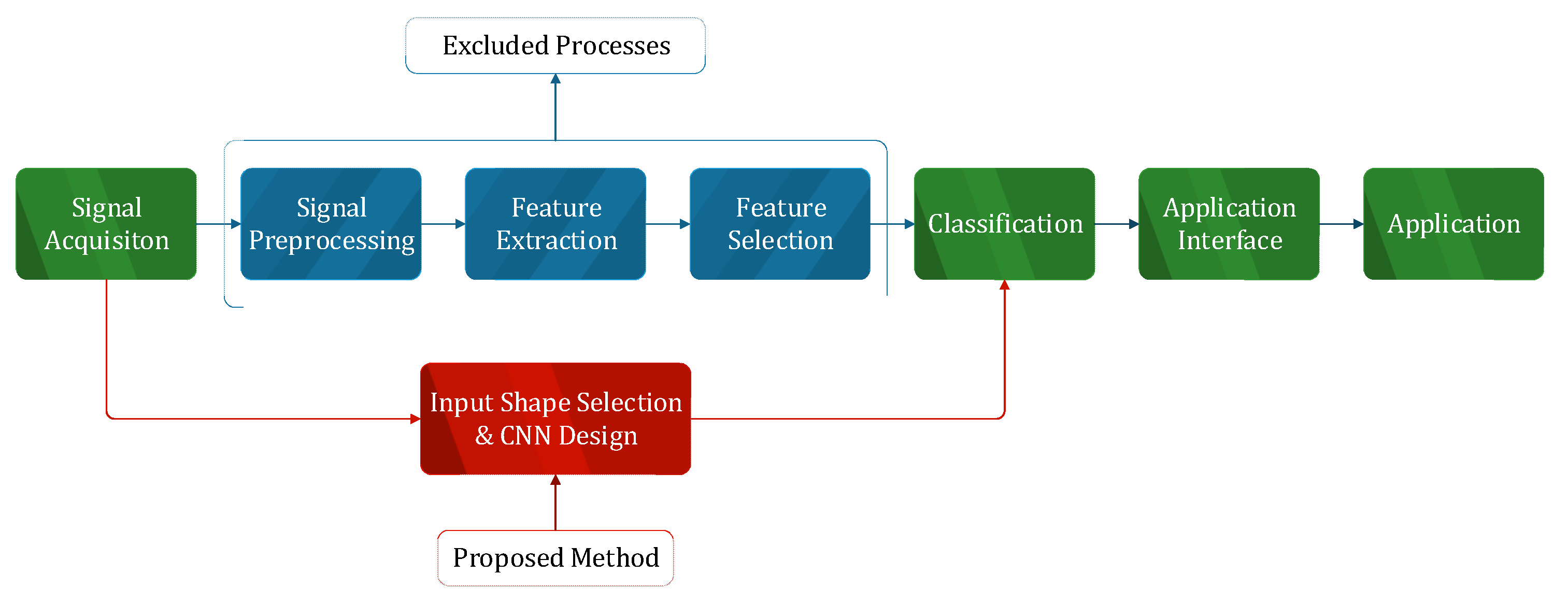
:1. Introduction
2. Dataset and Methods
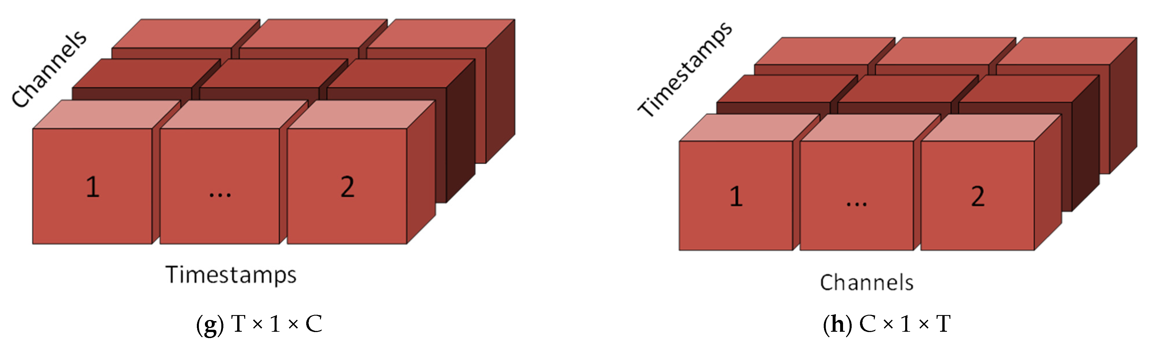
2.1. Input Shape
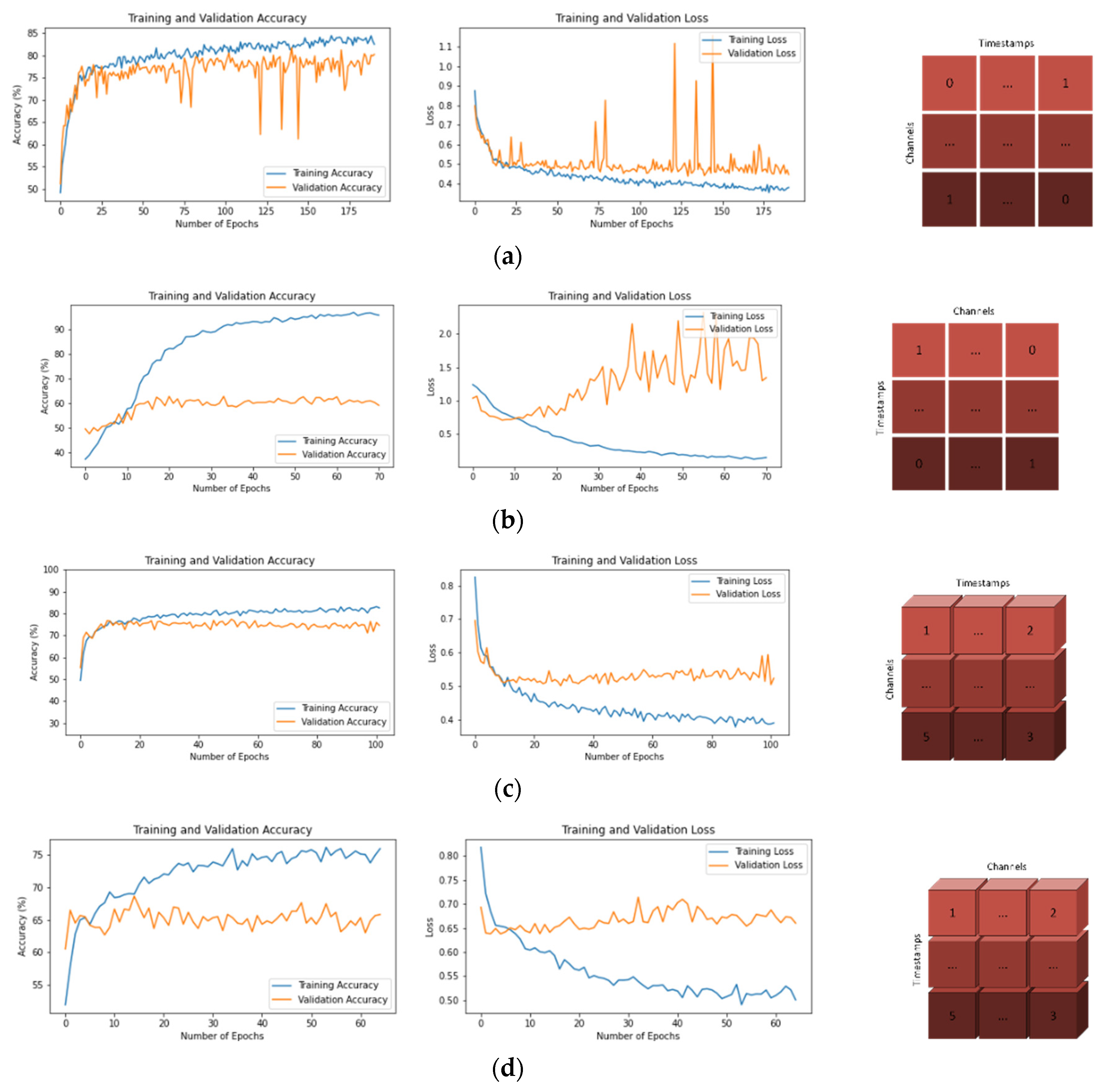
- (a)
- T × C
- (b)
- C × T
- (c)
- T × C × 1
- (d)
- C × T × 1
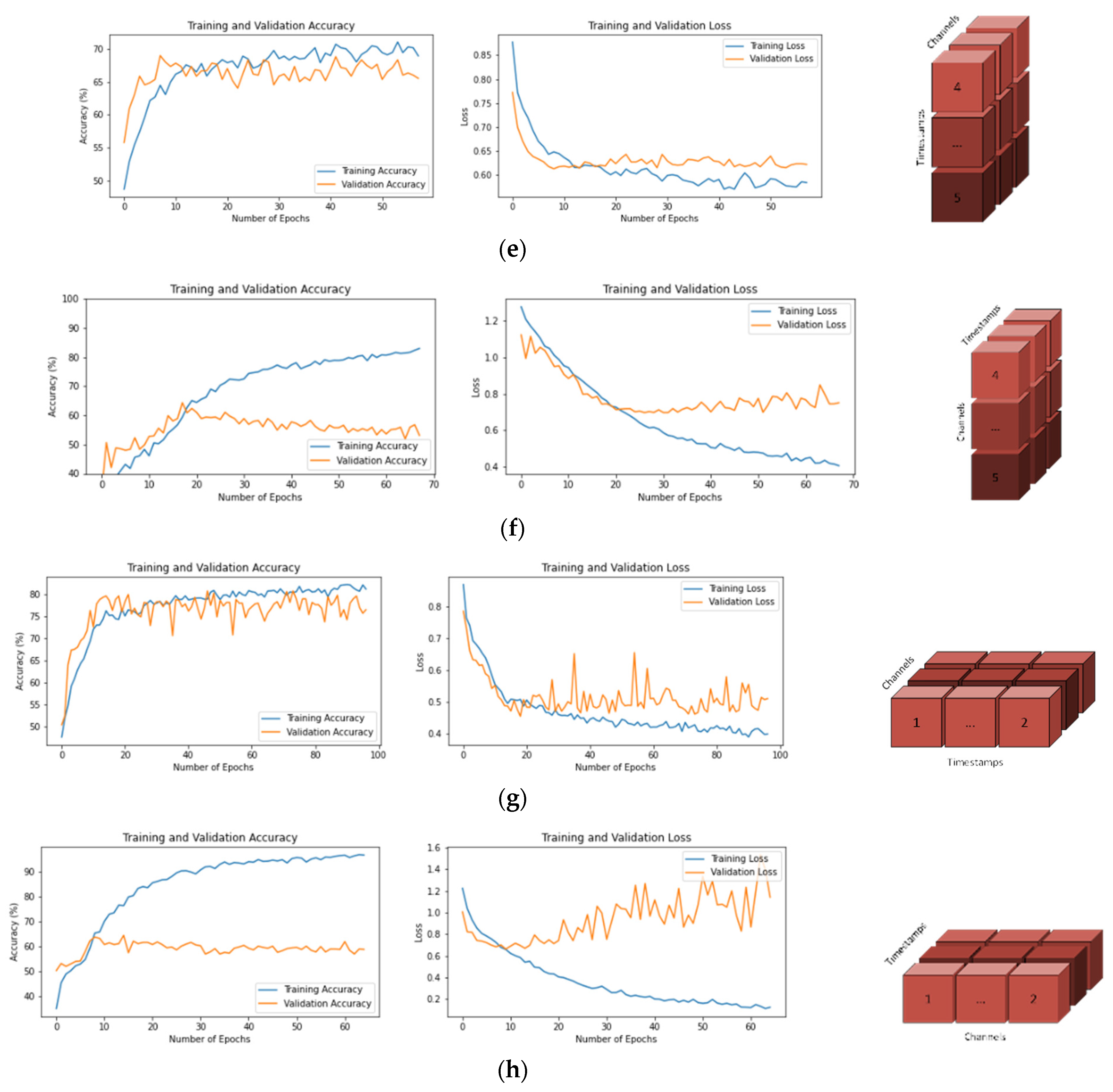
- (e)
- 1 × T × C
- (f)
- 1 × C × T
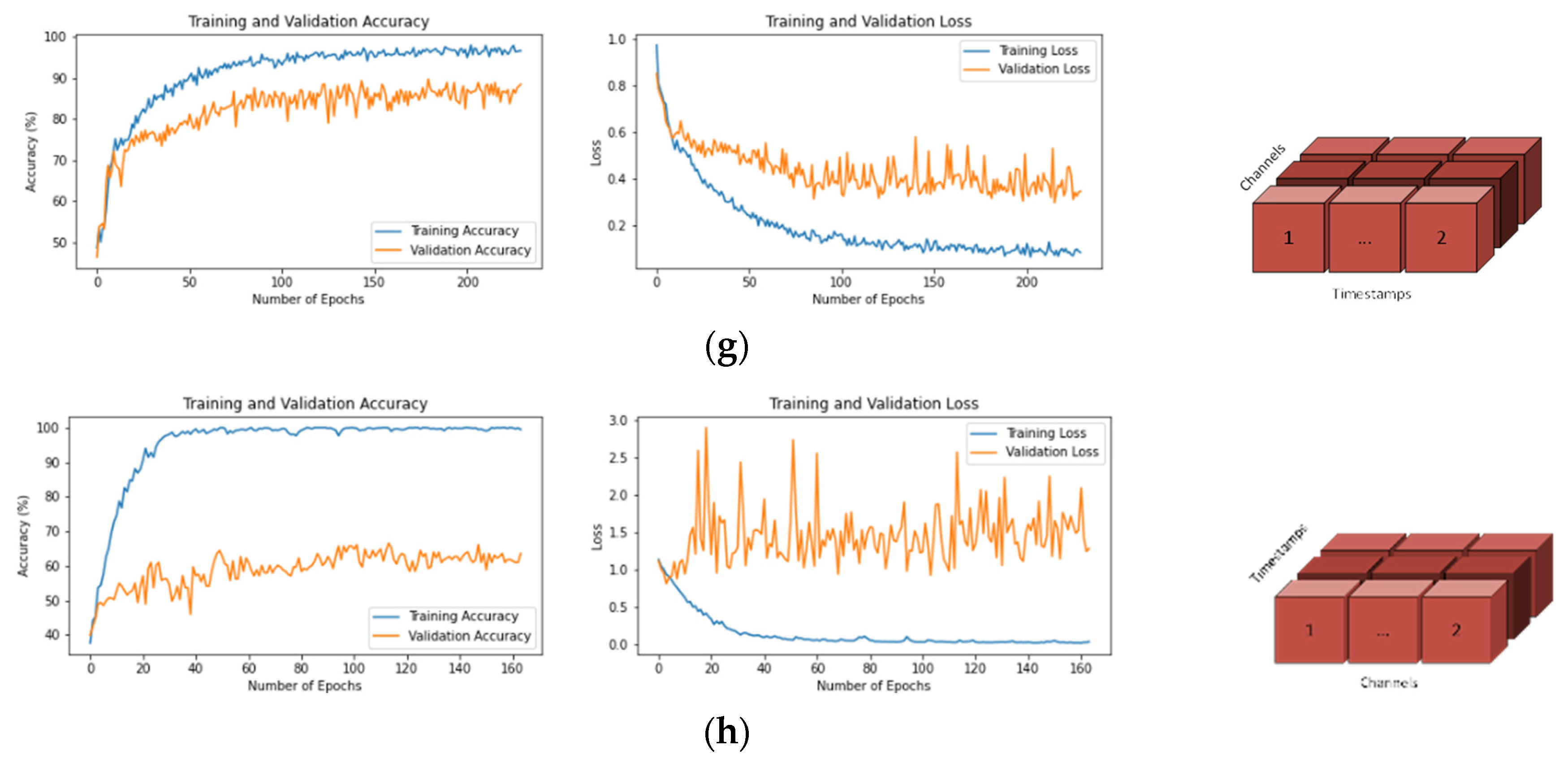
- (g)
- T × 1 × C
- (h)
- C × 1 × T
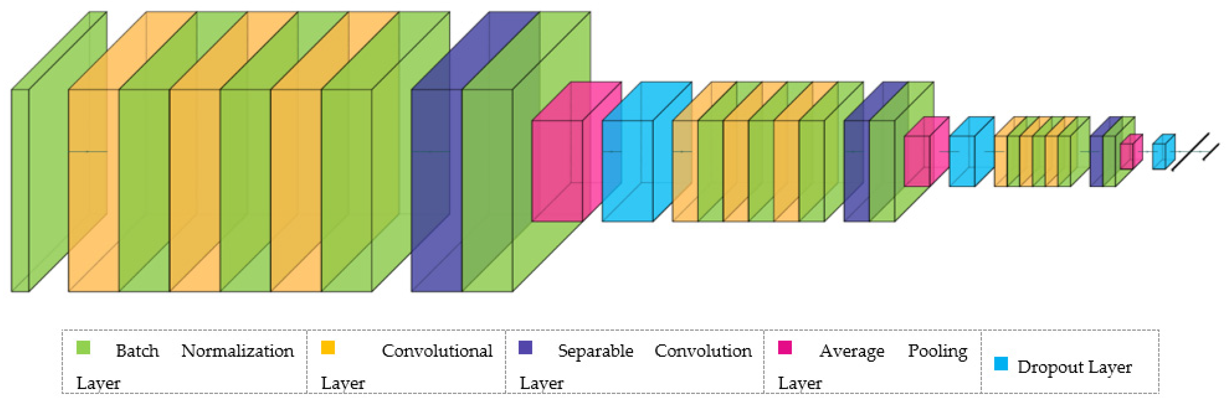
2.2. Proposed CNN Model
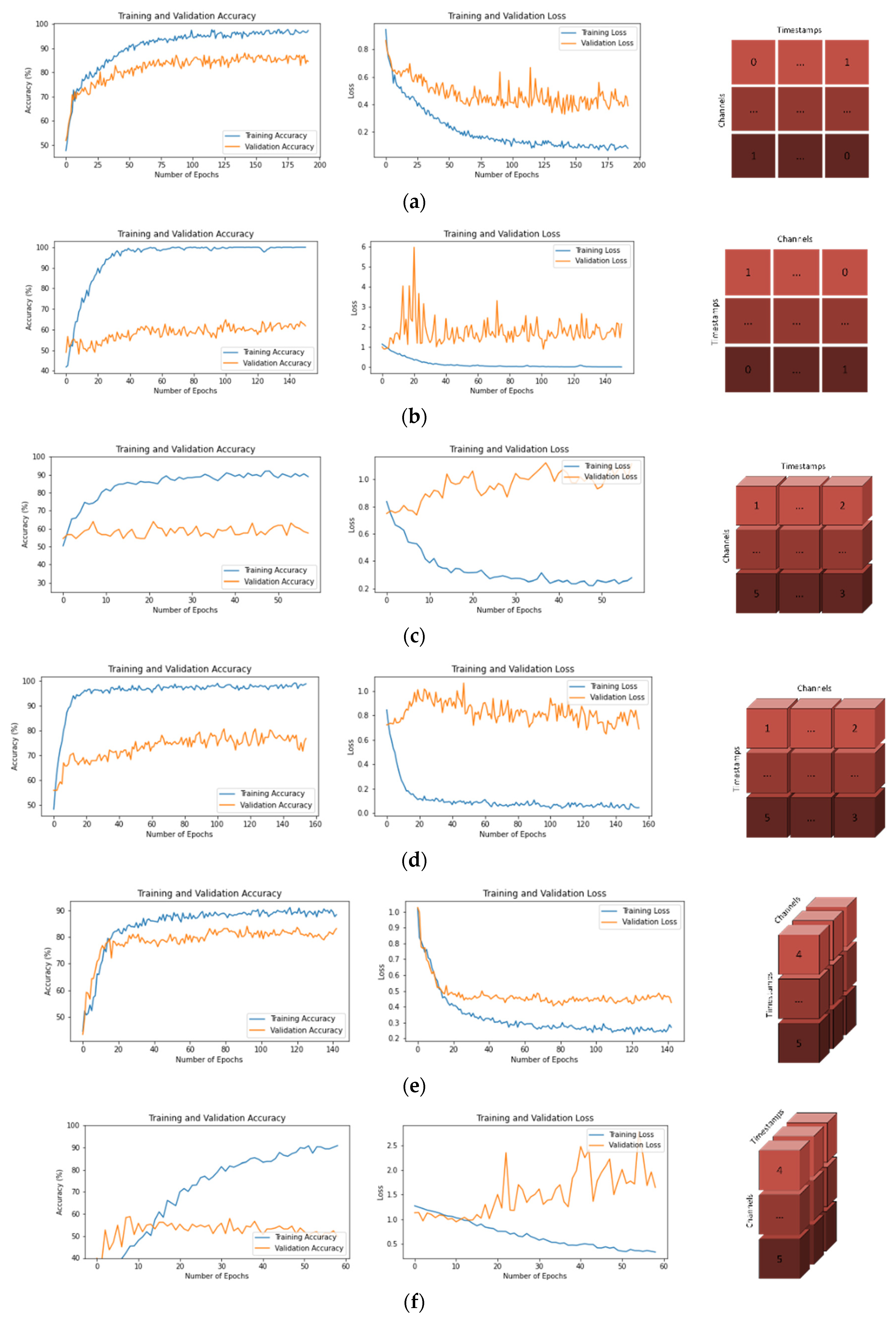
3. Experimental Results
3.1. Training and Validation Graphs
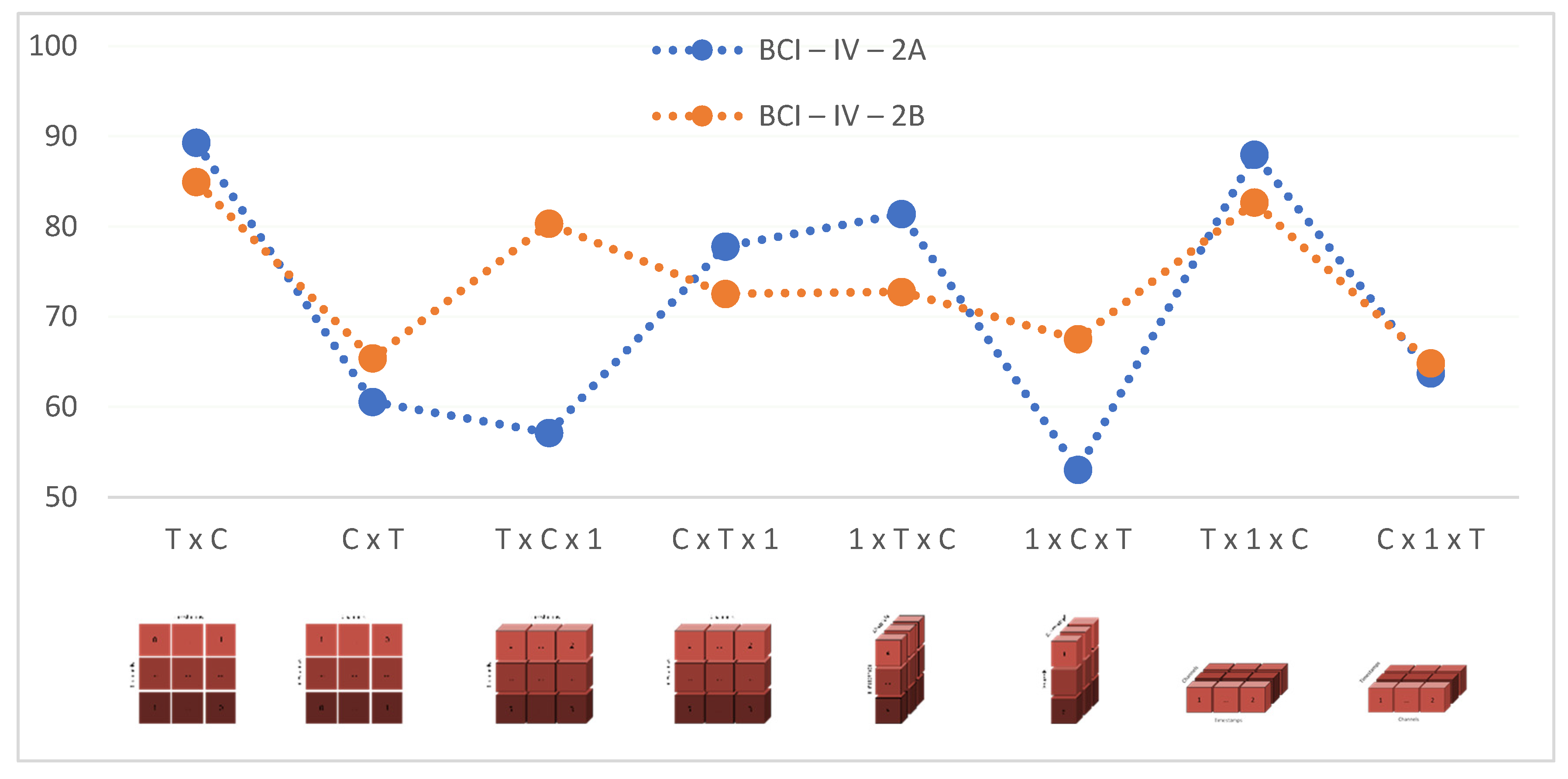
3.2. Accuracy Values
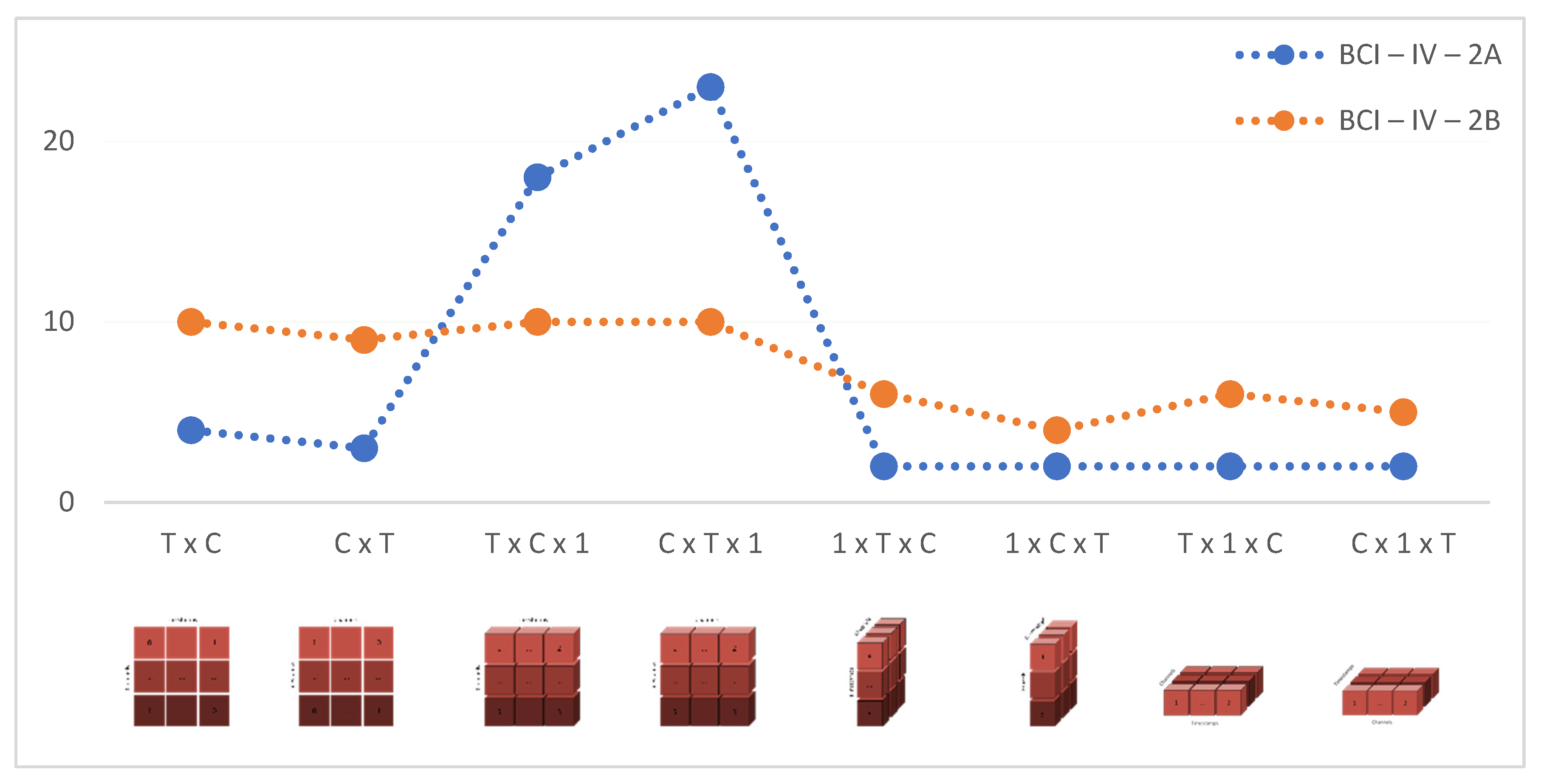
3.3. Epoch Times
3.4. Confusion Matrices
3.5. Model Statistics
4. Discussion
5. Conclusions
Author Contributions
Funding
Institutional Review Board Statement
Informed Consent Statement
Data Availability Statement
Conflicts of Interest
References
- Gannouni, S.; Belwafi, K.; Al-Sulmi, M.R.; Al-Farhood, M.D.; Al-Obaid, O.A.; Al-Awadh, A.M.; Aboalsamh, H.; Belghith, A. A Brain Controlled Command-Line Interface to Enhance the Accessibility of Severe Motor Disabled People to Personnel Computer. Brain Sci. 2022, 12, 926. [Google Scholar] [CrossRef]
- Abualsaud, K.; Mahmuddin, M.; Saleh, M.; Mohamed, A. Ensemble Classifier for Epileptic Seizure Detection for Imperfect EEG Data. Sci. World J. 2015, 2015, 945689. [Google Scholar] [CrossRef]
- Tsui, C.; Gan, J.; Hu, H. A Self-Paced Motor Imagery Based Brain-Computer Interface for Robotic Wheelchair Control. Clin. EEG Neurosci. 2011, 42, 225–229. [Google Scholar] [CrossRef]
- Bonnet, L.; Lotte, F.; Lecuyer, A. Two Brains, One Game: Design and Evaluation of a Multiuser BCI Video Game Based on Motor Imagery. IEEE Trans. Comput. Intell. AI Games 2013, 5, 185–198. [Google Scholar] [CrossRef] [Green Version]
- Heo, J.; Yoon, G. EEG Studies on Physical Discomforts Induced by Virtual Reality Gaming. J. Electr. Eng. Technol. 2020, 15, 1323–1329. [Google Scholar] [CrossRef]
- Ng, D.W.; Soh, Y.; Goh, S. Development of an autonomous BCI wheelchair. In Proceedings of the 2014 IEEE Symposium on Computational Intelligence in Brain Computer Interfaces (CIBCI), Orlando, FL, USA, 9–12 December 2014. [Google Scholar]
- Cao, L.; Wu, H.; Chen, S.; Dong, Y.; Zhu, C.; Jia, J.; Fan, C. A Novel Deep Learning Method Based on an Overlapping Time Window Strategy for Brain–Computer Interface-Based Stroke Rehabilitation. Brain Sci. 2022, 12, 1502. [Google Scholar] [CrossRef] [PubMed]
- Aldayel, M.; Ykhlef, M.; Al-Nafjan, A. Deep Learning for EEG-Based Preference Classification in Neuromarketing. Appl. Sci. 2020, 10, 1525. [Google Scholar] [CrossRef] [Green Version]
- Bhagat, N.A.; Venkatakrishnan, A.; Abibullaev, B.; Artz, E.J.; Yozbatiran, N.; Blank, A.A.; French, J.; Karmonik, C.; Grossman, R.G.; O’Malley, M.K.; et al. Design and Optimization of an EEG-Based Brain Machine Interface (BMI) to an Upper-Limb Exoskeleton for Stroke Survivors. Front. Neurosci. 2016, 10, 122. [Google Scholar] [CrossRef] [PubMed] [Green Version]
- van de Laar, B.; Gurkok, H.; Bos, D.P.-O.; Poel, M.; Nijholt, A. Experiencing BCI Control in a Popular Computer Game. IEEE Trans. Comput. Intell. AI Games 2013, 5, 176–184. [Google Scholar] [CrossRef]
- He, Y.; Eguren, D.; Azorín, J.; Grossman, R.; Luu, T.; Contreras-Vidal, J. Brain–machine interfaces for controlling lower-limb powered robotic systems. J. Neural Eng. 2018, 15, 021004. [Google Scholar] [CrossRef]
- Pires, G.; Torres, M.; Casaleiro, N.; Nunes, U.; Castelo-Branco, M. Playing Tetris with non-invasive BCI. In Proceedings of the 2011 IEEE 1st International Conference on Serious Games and Applications for Health (SeGAH), Braga, Portugal, 16–18 November 2011. [Google Scholar]
- Rezeika, A.; Benda, M.; Stawicki, P.; Gembler, F.; Saboor, A.; Volosyak, I. Brain–Computer Interface Spellers: A Review. Brain Sci. 2018, 8, 57. [Google Scholar] [CrossRef] [PubMed] [Green Version]
- Zhu, X.; Li, P.; Li, C.; Yao, D.; Zhang, R.; Xu, P. Separated channel convolutional neural network to realize the training free motor imagery BCI systems. Biomed. Signal Process. Control 2019, 49, 396–403. [Google Scholar] [CrossRef]
- Alazrai, R.; Abuhijleh, M.; Alwanni, H.; Daoud, M. A Deep Learning Framework for Decoding Motor Imagery Tasks of the Same Hand Using EEG Signals. IEEE Access 2019, 7, 109612–109627. [Google Scholar] [CrossRef]
- Procházka, A.; Kukal, J.; Vyšata, O. Wavelet transform use for feature extraction and EEG signal segments classification. In Proceedings of the 2008 3rd International Symposium on Communications, Control and Signal Processing, Saint Julian’s, Malta, 12–14 March 2008; pp. 719–722. [Google Scholar]
- Edelman, B.; Baxter, B.; He, B. EEG Source Imaging Enhances the Decoding of Complex Right-Hand Motor Imagery Tasks. IEEE Trans. Biomed. Eng. 2016, 63, 4–14. [Google Scholar] [CrossRef]
- Zabidi, A.; Mansor, W.; Lee, Y.K.; Che Wan Fadzal CW, N.F. Short-time Fourier Transform analysis of EEG signal generated during imagined writing. In Proceedings of the 2012 International Conference on System Engineering and Technology (ICSET), Bandung, Indonesia, 11–12 September 2012; pp. 12–15. [Google Scholar]
- Tabar, Y.; Halici, U. A novel deep learning approach for classification of EEG motor imagery signals. J. Neural Eng. 2016, 14, 016003. [Google Scholar] [CrossRef]
- Luo, J.; Feng, Z.; Zhang, J.; Lu, N. Dynamic frequency feature selection based approach for classification of motor imageries. Comput. Biol. Med. 2016, 75, 45–53. [Google Scholar] [CrossRef] [PubMed]
- Lee, H.; Choi, Y. Application of Continuous Wavelet Transform and Convolutional Neural Network in Decoding Motor Imagery Brain-Computer Interface. Entropy 2019, 21, 1199. [Google Scholar] [CrossRef] [Green Version]
- Meng, J.; Zhang, S.; Bekyo, A.; Olsoe, J.; Baxter, B.; He, B. Noninvasive Electroencephalogram Based Control of a Robotic Arm for Reach and Grasp Tasks. Sci. Rep. 2016, 6, 38565. [Google Scholar] [CrossRef] [Green Version]
- Saa, J.; Çetin, M. A latent discriminative model-based approach for classification of imaginary motor tasks from EEG data. J. Neural Eng. 2012, 9, 026020. [Google Scholar] [CrossRef] [PubMed] [Green Version]
- Li, M.; Zhu, W.; Liu, H.; Yang, J. Adaptive Feature Extraction of Motor Imagery EEG with Optimal Wavelet Packets and SE-Isomap. Appl. Sci. 2017, 7, 390. [Google Scholar] [CrossRef]
- Ang, K.K.; Chin, Z.Y.; Zhang, H.; Guan, C. Filter Bank Common Spatial Pattern (FBCSP) in brain-computer interface. In Proceedings of the 2008 IEEE International Joint Conference on Neural Networks (IEEE World Congress on Computational Intelligence), Hong Kong, China, 1–8 June 2008; pp. 2390–2397. [Google Scholar]
- Lu, N.; Li, T.; Ren, X.; Miao, H. A Deep Learning Scheme for Motor Imagery Classification based on Restricted Boltzmann Machines. IEEE Trans. Neural Syst. Rehabil. Eng. 2017, 25, 566–576. [Google Scholar] [CrossRef] [PubMed]
- Sciaraffa, N.; Di Flumeri, G.; Germano, D.; Giorgi, A.; Di Florio, A.; Borghini, G.; Vozzi, A.; Ronca, V.; Varga, R.; van Gasteren, M.; et al. Validation of a Light EEG-Based Measure for Real-Time Stress Monitoring during Realistic Driving. Brain Sci. 2022, 12, 304. [Google Scholar] [CrossRef]
- He, H.; Wu, D. Transfer Learning for Brain–Computer Interfaces: A Euclidean Space Data Alignment Approach. IEEE Trans. Biomed. Eng. 2020, 67, 399–410. [Google Scholar] [CrossRef] [Green Version]
- Al-Saegh, A.; Dawwd, S.; Abdul-Jabbar, J. Deep learning for motor imagery EEG-based classification: A review. Biomed. Signal Process. Control. 2021, 63, 102172. [Google Scholar] [CrossRef]
- Lashgari, E.; Ott, J.; Connelly, A.; Baldi, P.; Maoz, U. An end-to-end CNN with attentional mechanism applied to raw EEG in a BCI classification task. J. Neural Eng. 2021, 18, 0460e3. [Google Scholar] [CrossRef]
- Yang, B.; Duan, K.; Fan, C.; Hu, C.; Wang, J. Automatic ocular artifacts removal in EEG using deep learning. Biomed. Signal Process. Control 2018, 43, 148–158. [Google Scholar] [CrossRef]
- Dai, G.; Zhou, J.; Huang, J.; Wang, N. HS-CNN: A CNN with hybrid convolution scale for EEG motor imagery classification. J. Neural Eng. 2020, 17, 016025. [Google Scholar] [CrossRef]
- Zhang, C.; Kim, Y.K.; Eskandarian, A. EEG-inception: An accurate and robust end-to-end neural network for EEG-based motor imagery classification. J. Neural Eng. 2021, 18, 046014. [Google Scholar] [CrossRef]
- Alotaiby, T.; El-Samie, F.E.A.; Alshebeili, S.A.; Ahmad, I. A review of channel selection algorithms for EEG signal processing. EURASIP J. Adv. Signal Process 2015, 2015, 66. [Google Scholar] [CrossRef] [Green Version]
- da Cruz, J.R.; Chicherov, V.; Herzog, M.H.; Figueiredo, P. An automatic pre-processing pipeline for EEG analysis (APP) based on robust statistics. Clin. Neurophysiol. 2018, 129, 1427–1437. [Google Scholar] [CrossRef]
- Mashhadi, N.; Khuzani, A.; Heidari, M.; Khaledyan, D. Deep learning denoising for EOG artifacts removal from EEG signals. In Proceedings of the 2020 IEEE Global Humanitarian Technology Conference (GHTC), Seattle, WA, USA, 29 October–1 November 2020; pp. 1–6. [Google Scholar] [CrossRef]
- Val-Calvo, M.; Álvarez-Sánchez, J.R.; Ferrández-Vicente, J.M.; Fernández, E. Optimization of Real-Time EEG Artifact Removal and Emotion Estimation for Human-Robot Interaction Applications. Front. Comput. Neurosci. 2019, 13, 80. [Google Scholar] [CrossRef] [PubMed] [Green Version]
- Lun, X.; Yu, Z.; Chen, T.; Wang, F.; Hou, Y. A Simplified CNN Classification Method for MI-EEG via the Electrode Pairs Signals. Front. Hum. Neurosci. 2020, 14, 338. [Google Scholar] [CrossRef]
- Dose, H.; Møller, J.S.; Iversen, H.K.; Puthusserypady, S. An end-toend deep learning approach to MI-EEG signal classification for BCIs. Expert Syst. Appl. 2018, 114, 532–542. [Google Scholar] [CrossRef]
- Hajinoroozi, M.; Mao, Z.; Jung, T.-P.; Lin, C.-T.; Huang, Y. EEG-based prediction of driver’s cognitive performance by deep convolutional neural network. Signal Process. 2016, 47, 549–555. [Google Scholar] [CrossRef]
- Shen, Y.; Lu, H.; Jia, J. Classification of motor imagery EEG signals with deep learning models. In Proceedings of the International Conference on Intelligent Science and Big Data Engineering, Dalian, China, 22–23 September 2017; pp. 181–190. [Google Scholar] [CrossRef]
- Schirrmeister, R.T.; Springenberg, J.T.; Fiederer, L.D.J.; Glasstetter, M.; Eggensperger, K.; Tangermann, M.; Hutter, F.; Burgard, W.; Ball, T. Deep learning with convolutional neural networks for EEGdecoding and visualization. Hum. Brain Mapp. 2017, 38, 5391–5420. [Google Scholar] [CrossRef] [Green Version]
- Raza, H.; Rathee, D.; Zhou, S.M.; Cecotti, H.; Prasad, G. Covariate shift estimation based adaptive ensemble learning for handling non-stationarity in motor imagery related EEG-based brain-computer interface. Neurocomputing 2019, 343, 154–166. [Google Scholar] [CrossRef]
- Sugiyama, M.; Krauledat, M.; Müller, K. Covariate shift adaptation by importance weighted cross validation. J. Mach. Learn. Res. 2007, 8, 985–1005. [Google Scholar]
- Pan, S.; Yang, Q. A survey on transfer learning. IEEE Trans. Knowl. Data Eng. 2010, 22, 1345–1359. [Google Scholar] [CrossRef]
- Miladinović, A.; Ajčević, M.; Jarmolowska, J.; Marusic, U.; Colussi, M.; Silveri, G.; Battaglini, P.P.; Accardo, A. Effect of power feature covariance shift on BCI spatial-filtering techniques: A comparative study. Comput. Methods Programs Biomed. 2021, 198, 105808. [Google Scholar] [CrossRef]
- Ioffe, S.; Szegedy, C. Batch normalization: Accelerating deep network training by reducing internal covariate shift. In Proceedings of the 32nd International Conference on Machine Learning, Lille, France, 6–11 July 2015; pp. 448–456. [Google Scholar]
- Brunner, C.; Leeb, R.; Müller-Putz, G.; Schlögl, A.; Pfurtscheller, G. BCI Competition 2008—Graz Data Sets 2A and 2B (Graz: Institute for Knowledge Discovery). Available online: http://bbci.de/competition/iv/ (accessed on 1 June 2022).
- Wang, S.; Liu, W.; Wu, J.; Cao, L.; Meng, Q.; Kennedy, P.J. Training deep neural networks on imbalanced data sets. In Proceedings of the 2016 International Joint Conference on Neural Networks (IJCNN), Vancouver, BC, Canada, 24–29 July 2016. [Google Scholar]
- Zhang, C.; Bengio, S.; Hardt, M.; Recht, B.; Vinyals, O. Understanding deep learning requires rethinking generalization. arXiv 2016, arXiv:1611.03530. [Google Scholar] [CrossRef]
- Zhang, Z.; Duan, F.; Sole-Casals, J.; Dinares-Ferran, J.; Cichocki, A.; Yang, Z.; Sun, Z. A novel deep learning approach with data augmentation to classify motor imagery signals. IEEE Access 2019, 7, 15945. [Google Scholar] [CrossRef]
- McFarland, D.J.; Sarnacki, W.; Wolpaw, J. Electroencephalographic (EEG) control of three dimensional movement. J. Neural Eng. 2010, 7, 036007. [Google Scholar] [CrossRef] [Green Version]
- Suwannarat, A.; Pan-ngum, S.; Israsena, P. Comparison of EEG measurement of upper limb movement in motor imagery training system. Biomed. Eng. Online 2018, 17, 103. [Google Scholar] [CrossRef] [Green Version]
- Gaur, P.; Pachori, R.B.; Wang, H.; Prasad, G. An empirical mode decomposition based filtering method for classification of motor-imagery EEG signals for enhancing brain-computer interface. In Proceedings of the 2015 International Joint Conference on Neural Networks (IJCNN), Killarney, Ireland, 12–17 July 2015. [Google Scholar]
- Sakhavi, S.; Guan, C.; Yan, S. Learning Temporal Information for Brain-Computer Interface Using Convolutional Neural Networks. IEEE Trans. Neural Netw. Learn. Syst. 2018, 29, 5619–5629. [Google Scholar] [CrossRef] [PubMed]
- Ang, K.; Chin, Z.; Wang, C.; Guan, C.; Zhang, H. Filter Bank Common Spatial Pattern Algorithm on BCI Competition IV Datasets 2a and 2b. Front. Neurosci. 2012, 6, 39. [Google Scholar] [CrossRef] [PubMed] [Green Version]
- Mane, R.; Chew, E.; Chua, K.; Ang, K.K.; Robinson, N.; Vinod, A.P.; Lee, S.-W.; Guan, C. FBCNet: A multi-view convolutional neural network for brain-computer interface. arXiv 2021, arXiv:2104.01233. [Google Scholar]
- Liu, T.; Yang, D. A Densely Connected Multi-Branch 3D Convolutional Neural Network for Motor Imagery EEG Decoding. Brain Sci. 2021, 11, 197. [Google Scholar] [CrossRef] [PubMed]
- Jiang, Q.; Zhang, Y.; Zheng, K. Motor Imagery Classification via Kernel-Based Domain Adaptation on an SPD Manifold. Brain Sci. 2022, 12, 659. [Google Scholar] [CrossRef]
- Gao, S.; Yang, J.; Shen, T.; Jiang, W. A Parallel Feature Fusion Network Combining GRU and CNN for Motor Imagery EEG Decoding. Brain Sci. 2022, 12, 1233. [Google Scholar] [CrossRef]


| T × C | C × T | T × C × 1 | C × T × 1 | 1 × T × C | 1 × C × T | T × 1 × C | C × 1 × T | |
|---|---|---|---|---|---|---|---|---|
| S1 | 84.40 | 60.28 | 54.61 | 63.12 | 68.09 | 47.52 | 81.56 | 60.28 |
| S2 | 78.87 | 54.23 | 51.41 | 72.54 | 80.28 | 51.41 | 81.69 | 58.45 |
| S3 | 96.35 | 54.74 | 48.18 | 71.53 | 75.18 | 51.82 | 88.32 | 59.12 |
| S4 | 88.79 | 61.21 | 60.34 | 79.31 | 81.90 | 51.72 | 84.48 | 64.66 |
| S5 | 92.59 | 72.59 | 68.15 | 87.41 | 94.07 | 57.04 | 96.30 | 74.81 |
| S6 | 84.26 | 59.26 | 56.48 | 74.07 | 80.56 | 50.00 | 83.33 | 62.04 |
| S7 | 92.14 | 72.14 | 65.00 | 91.43 | 85.71 | 56.43 | 93.57 | 74.29 |
| S8 | 97.76 | 55.97 | 55.97 | 79.10 | 84.33 | 55.22 | 94.03 | 59.70 |
| S9 | 88.46 | 54.62 | 53.85 | 81.54 | 82.31 | 56.15 | 88.46 | 60.00 |
| Average | 89.29 | 60.56 | 57.11 | 77.78 | 81.38 | 53.03 | 87.97 | 63.71 |
| STD | 5.47 | 6.41 | 5.70 | 7.70 | 6.38 | 2.96 | 5.02 | 5.74 |
| T × C | C × T | T × C × 1 | C × T × 1 | 1 × T × C | 1 × C × T | T × 1 × C | C × 1 × T | |
|---|---|---|---|---|---|---|---|---|
| S1 | 78.95 | 62.72 | 70.61 | 64.91 | 63.16 | 59.65 | 78.95 | 61.40 |
| S2 | 70.20 | 56.73 | 63.67 | 71.43 | 64.49 | 66.53 | 64.49 | 61.63 |
| S3 | 73.48 | 60.87 | 67.39 | 68.70 | 76.09 | 67.83 | 66.96 | 58.70 |
| S4 | 96.74 | 57.33 | 94.14 | 64.17 | 61.56 | 58.96 | 94.79 | 58.31 |
| S5 | 96.70 | 93.04 | 92.31 | 95.24 | 97.07 | 93.77 | 98.53 | 89.01 |
| S6 | 83.67 | 60.96 | 76.10 | 69.32 | 68.53 | 64.14 | 78.09 | 61.35 |
| S7 | 90.09 | 80.60 | 87.93 | 81.47 | 89.66 | 82.76 | 93.10 | 76.72 |
| S8 | 91.74 | 64.35 | 88.26 | 81.30 | 78.26 | 62.61 | 89.57 | 62.17 |
| S9 | 82.86 | 51.84 | 82.45 | 56.33 | 55.92 | 51.43 | 79.59 | 54.29 |
| Average | 84.94 | 65.38 | 80.32 | 72.54 | 72.75 | 67.52 | 82.67 | 64.84 |
| STD | 8.61 | 11.70 | 10.08 | 10.44 | 12.27 | 11.63 | 10.85 | 9.79 |
| Input Shape | Epoch Time (Second/Epoch) | |
|---|---|---|
| BCI-IV-2A | BCI-IV-2B | |
| T × C | 4 | 10 |
| C × T | 3 | 9 |
| T × C × 1 | 18 | 10 |
| C × T × 1 | 23 | 10 |
| 1 × T × C | 2 | 6 |
| 1 × C × T | 2 | 4 |
| T × 1 × C | 2 | 6 |
| C × 1 × T | 2 | 5 |
| Input Shape | BCI-IV-2A | BCI-IV-2B | ||||||
|---|---|---|---|---|---|---|---|---|
| TL | FL | TR | FR | TL | FL | TR | FR | |
| T × C | 536/593 (90.4%) | 57 | 521/590 | 69 | 936/1118 (83.7%) | 182 | 979/1123 | 144 |
| (9.6%) | (88.3%) | (11.7%) | (16.3%) | (87.2%) | (12.8%) | |||
| C × T | 384/593 (64.8%) | 209 | 333/590 | 257 | 665/1118 (59.5%) | 453 | 802/1123 | 321 |
| (35.2%) | (56.4%) | (43.6%) | (40.5%) | (71.4%) | (28.6%) | |||
| T × C × 1 | 314/593 (53.0%) | 279 | 361/590 | 229 | 931/1118 (83.3%) | 187 | 882/1123 | 241 |
| (47.0%) | (61.2%) | (38.8%) | (16.7%) | (78.5%) | (21.5%) | |||
| C × T × 1 | 440/593 (74.2%) | 153 | 480/590 | 110 | 749/1118 (67.0%) | 369 | 877/1123 | 246 |
| (25.8%) | (81.4%) | (18.6%) | (33.0%) | (78.1%) | (21.9%) | |||
| 1 × T × C | 481/593 (81.1%) | 112 | 481/590 | 109 | 805/1118 (72.0%) | 313 | 823/1123 | 300 |
| (18.9%) | (81.5%) | (18.5%) | (28.0%) | (73.3%) | (26.7%) | |||
| 1 × C × T | 329/593 (55.5%) | 264 | 299/590 | 291 | 675/1118 (60.4%) | 443 | 840/1123 | 283 |
| (44.5%) | (50.7%) | (49.3%) | (39.6%) | (74.8%) | (25.2%) | |||
| T × 1 × C | 514/593 (86.7%) | 79 | 528/590 | 62 | 876/1118 (78.4%) | 242 | 989/1123 | 134 |
| (13.3%) | (89.5%) | (10.5%) | (21.6%) | (88.1%) | (11.9%) | |||
| C × 1 × T | 378/593 (63.7%) | 215 | 376/590 | 214 | 610/1118 (54.6%) | 508 | 846/1123 | 277 |
| (36.3%) | (63.7%) | (36.3%) | (45.4%) | (75.3%) | (24.7%) | |||
| Input Shape | BCI-IV-2A | BCI-IV-2B | ||||||
|---|---|---|---|---|---|---|---|---|
| Accuracy | F1 Score | Kappa | STD | Accuracy | F1 Score | Kappa | STD | |
| T × C | 89.293 | 0.893 | 0.787 | 5.471 | 84.943 | 0.854 | 0.709 | 8.607 |
| C × T | 60.561 | 0.605 | 0.212 | 6.413 | 65.383 | 0.653 | 0.309 | 11.695 |
| T × C × 1 | 57.114 | 0.570 | 0.141 | 5.704 | 80.318 | 0.809 | 0.618 | 10.083 |
| C × T × 1 | 77.782 | 0.777 | 0.555 | 7.697 | 72.538 | 0.725 | 0.451 | 10.436 |
| 1 × T × C | 81.376 | 0.813 | 0.626 | 6.376 | 72.747 | 0.726 | 0.453 | 12.269 |
| 1 × C × T | 53.033 | 0.531 | 0.062 | 2.958 | 67.518 | 0.674 | 0.352 | 11.628 |
| T × 1 × C | 87.969 | 0.881 | 0.762 | 5.021 | 82.665 | 0.830 | 0.664 | 10.846 |
| C × 1 × T | 63.713 | 0.637 | 0.275 | 5.737 | 64.835 | 0.646 | 0.299 | 9.790 |
Disclaimer/Publisher’s Note: The statements, opinions and data contained in all publications are solely those of the individual author(s) and contributor(s) and not of MDPI and/or the editor(s). MDPI and/or the editor(s) disclaim responsibility for any injury to people or property resulting from any ideas, methods, instructions or products referred to in the content. |
© 2023 by the authors. Licensee MDPI, Basel, Switzerland. This article is an open access article distributed under the terms and conditions of the Creative Commons Attribution (CC BY) license (https://creativecommons.org/licenses/by/4.0/).
Share and Cite
Arı, E.; Taçgın, E. Input Shape Effect on Classification Performance of Raw EEG Motor Imagery Signals with Convolutional Neural Networks for Use in Brain—Computer Interfaces. Brain Sci. 2023, 13, 240. https://doi.org/10.3390/brainsci13020240
Arı E, Taçgın E. Input Shape Effect on Classification Performance of Raw EEG Motor Imagery Signals with Convolutional Neural Networks for Use in Brain—Computer Interfaces. Brain Sciences. 2023; 13(2):240. https://doi.org/10.3390/brainsci13020240
Chicago/Turabian StyleArı, Emre, and Ertuğrul Taçgın. 2023. "Input Shape Effect on Classification Performance of Raw EEG Motor Imagery Signals with Convolutional Neural Networks for Use in Brain—Computer Interfaces" Brain Sciences 13, no. 2: 240. https://doi.org/10.3390/brainsci13020240