

A REM Update Methodology Based on Clustering and Random Forest

Abstract
:1. Introduction
1.1. Related Work
1.2. Main Contributions
- We propose an efficient methodology to update a REM based on clustering and RF in a timely manner. In the proposed scheme, the K-means algorithm is applied to divide the area of interest in K clusters, where one RF model is deployed per cluster. The REM is constructed to cover every point within the area of interest, where the prediction of the RSSI values for each location is obtained by the corresponding RF model in each cluster.
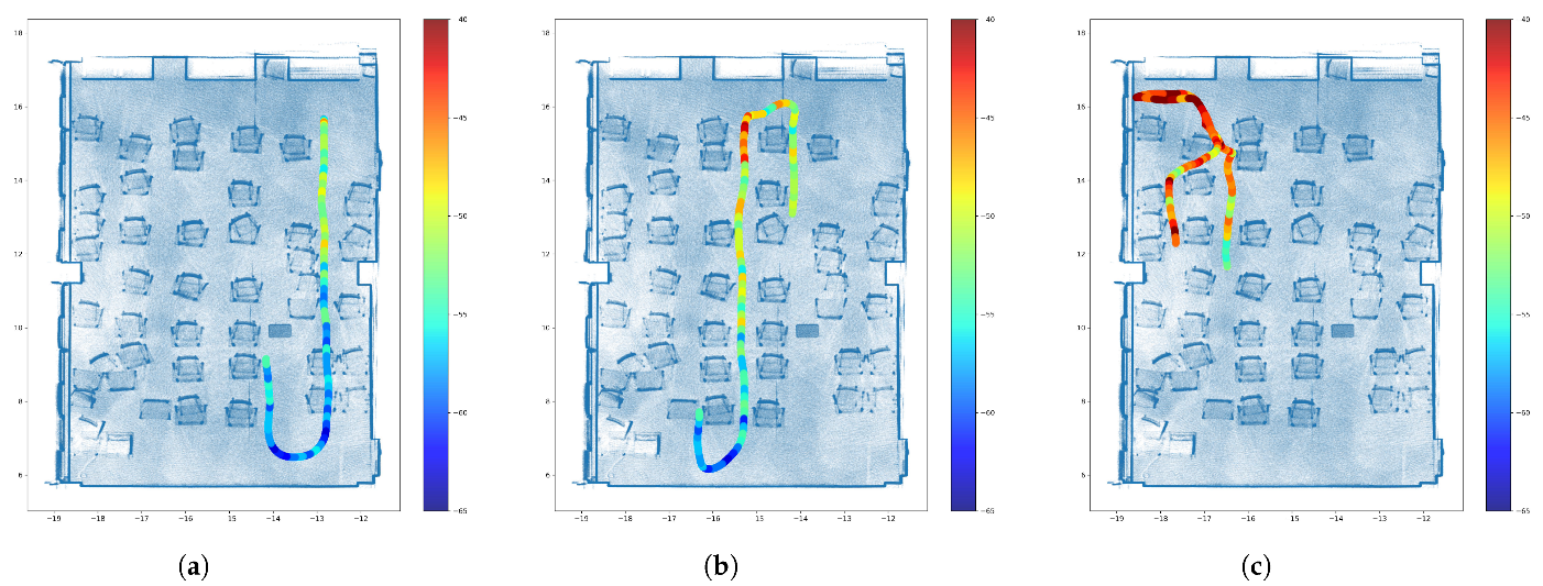
- The RSSI measurements were collected by a mobile robot, which can reduce the risk of human error because the robot can be programmed to move in a controlled manner. This can help ensure that RSSI measurements are taken at consistent intervals and under consistent conditions, while improving the accuracy and reliability of the measurements. Moreover, mobile robots can operate autonomously, which can save time and resources compared to manual data collection methods.
- In the REM construction, to avoid abrupt changes in the border areas between the clusters, we propose a methodology that utilizes the weighted average of the RF model predictions from the two nearest centroids to determine the RSSI value of the points within the border areas. Moreover, when new measurements are available, only the RF models for clusters that have enough measurement samples are updated.
- We extensively evaluate the proposed scheme for different scenarios, including the presence of obstacles and relocating the AP, and we consider several comparative ML methods, including the case without clusters. Moreover, the computational complexity of the proposed scheme is analyzed along with the comparative schemes. The simulation results demonstrated the superior performance of the proposed scheme compared to the baseline methods in effectively adapting to changes in the wireless environment. Moreover, the proposed approach requires only newly collected data in specific sectors to update a large area of interest.
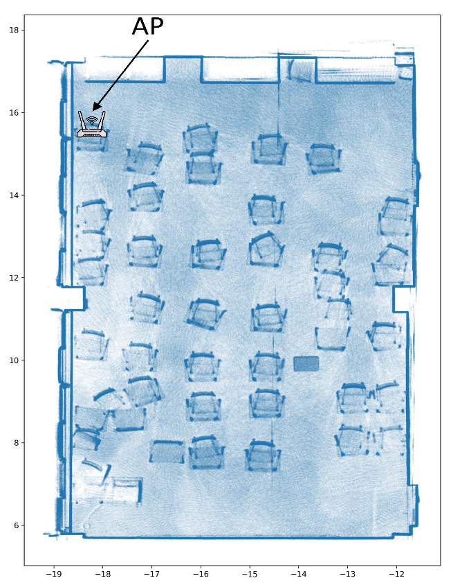
2. Measurement Methodology
3. Proposed Approach for REM Updates
3.1. Overview
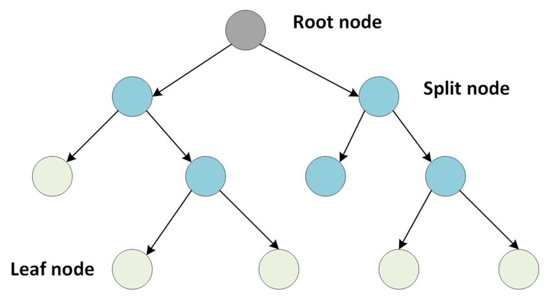
3.2. Random Forest
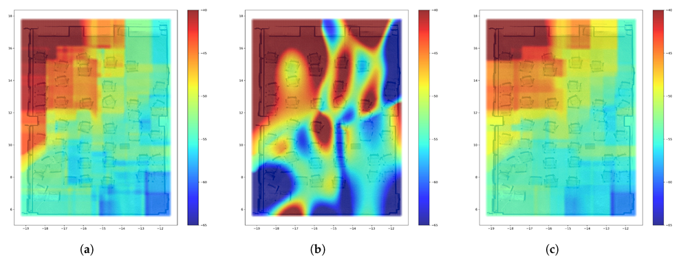
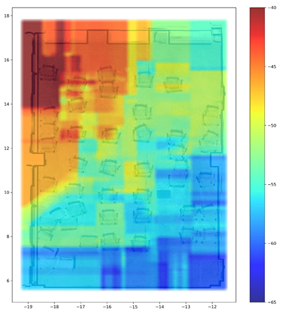
3.3. REM Construction
4. Evaluation
4.1. Historical Dataset and Comparative Models
4.2. REM Update Evaluation
5. Conclusions
Author Contributions
Funding
Institutional Review Board Statement
Informed Consent Statement
Data Availability Statement
Conflicts of Interest
References
- Chou, S.-F.; Yen, H.-W.; Pang, A.-C. A REM-Enabled Diagnostic Framework in Cellular-Based IoT Networks. IEEE Internet Things J. 2019, 6, 5273–5284. [Google Scholar] [CrossRef]
- Bi, S.; Lyu, J.; Ding, Z.; Zhang, R. Engineering Radio Maps for Wireless Resource Management. IEEE Wirel. Commun. 2019, 26, 133–141. [Google Scholar] [CrossRef]
- Garcia, C.E.; Camana, M.R.; Koo, I. Prediction of Digital Terrestrial Television Coverage Using Machine Learning Regression. IEEE Trans. Broadcast. 2019, 65, 702–712. [Google Scholar]
- Han, T.; Bozorgi, S.; Orang, A.; Hosseinabadi, A.; Sangaiah, A.; Chen, M.-Y. A Hybrid Unequal Clustering Based on Density with Energy Conservation in Wireless Nodes. Sustainability 2019, 11, 746. [Google Scholar] [CrossRef]
- Gallagher, T.; Li, B.; Dempster, A.G.; Rizos, C. Database updating through user feedback in fingerprint-based Wi-Fi location systems. In Proceedings of the 2010 Ubiquitous Positioning Indoor Navigation and Location Based Service, Kirkkonummi, Finland, 14–15 October 2010. [Google Scholar]
- Lim, J.-S.; Jang, W.-H.; Yoon, G.-W.; Han, D.-S. Radio Map Update Automation for WiFi Positioning Systems. IEEE Commun. Lett. 2013, 17, 693–696. [Google Scholar] [CrossRef]
- Luo, C.; Hong, H.; Chan, M.C.; Li, J.; Zhang, X.; Ming, Z. MPiLoc: Self-Calibrating Multi-Floor Indoor Localization Exploiting Participatory Sensing. IEEE Trans. Mob. Comput. 2018, 17, 141–154. [Google Scholar] [CrossRef]
- Liu, X.; Cen, J.; Zhan, Y.; Tang, C. An Adaptive Fingerprint Database Updating Method for Room Localization. IEEE Access 2019, 7, 42626–42638. [Google Scholar] [CrossRef]
- Wu, C.; Yang, Z.; Xiao, C. Automatic Radio Map Adaptation for Indoor Localization Using Smartphones. IEEE Trans. Mob. Comput. 2018, 17, 517–528. [Google Scholar] [CrossRef]
- Wu, C.; Yang, Z.; Xiao, C.; Yang, C.; Liu, Y.; Liu, M. Static power of mobile devices: Self-updating radio maps for wireless indoor localization. In Proceedings of the 2015 IEEE Conference on Computer Communications (INFOCOM), Hong Kong, China, 26 April–1 May 2015. [Google Scholar]
- Liu, X.; Cen, J.; Hu, H.; Yu, Z.; Huang, Y. A radio map self-updating algorithm based on mobile crowd sensing. J. Netw. Comput. Appl. 2021, 194, 103225. [Google Scholar] [CrossRef]
- Yang, B.; He, S.; Chan, S.-H.G. Updating Wireless Signal Map with Bayesian Compressive Sensing. In Proceedings of the 19th ACM International Conference on Modeling, Analysis and Simulation of Wireless and Mobile Systems, Malta, 13–17 November 2016. [Google Scholar]
- Katagiri, K.; Fujii, T. Radio Environment Map Updating Procedure Considering Change of Surrounding Environment. In Proceedings of the 2020 IEEE Wireless Communications and Networking Conference Workshops (WCNCW), Seoul, Republic of Korea, 6–9 April 2020. [Google Scholar]
- Zhen, P.; Zhang, B.; Xie, C.; Guo, D. A Radio Environment Map Updating Mechanism Based on an Attention Mechanism and Siamese Neural Networks. Sensors 2022, 22, 6797. [Google Scholar] [CrossRef] [PubMed]
- Zhao, J.; Gao, X.; Wang, X.; Li, C.; Song, M.; Sun, Q. An Efficient Radio Map Updating Algorithm based on K-Means and Gaussian Process Regression. J. Navig. 2018, 71, 1055–1068. [Google Scholar] [CrossRef]
- TurtleBot3 Manual, Open-Source Robotics Foundation, Mountain View, CA, USA. Available online: https://emanual.robotis.com/docs/en/platform/turtlebot3/overview/ (accessed on 20 February 2023).
- Khan, M.U.; Zaidi, S.A.A.; Ishtiaq, A.; Bukhari, S.U.R.; Samer, S.; Farman, A. A Comparative Survey of LiDAR-SLAM and LiDAR based Sensor Technologies. In Proceedings of the 2021 Mohammad Ali Jinnah University International Conference on Computing (MAJICC), Karachi, Pakistan, 15–17 July 2021. [Google Scholar]
- Hovermap Mapping and Autonomy Payload User Manual; Emesent (PTY) LTD: Milton, QLD, Australia, 2021.
- Na, S.; Xumin, L.; Yong, G. Research on k-means Clustering Algorithm: An Improved k-means Clustering Algorithm. In Proceedings of the 2010 Third International Symposium on Intelligent Information Technology and Security Informatics, Jian, China, 2–4 April 2010. [Google Scholar]
- Phan, H.; Maaß, M.; Mazu, R.; Mertins, A. Random regression forests for acoustic event detection and classification. IEEE/ACM Trans. Audio Speech Lang. Process. 2015, 23, 20–31. [Google Scholar] [CrossRef]
- Smola, A.J.; Schölkopf, B. A tutorial on support vector regression. Stat. Comput. 2004, 14, 199–222. [Google Scholar] [CrossRef]
- Aggarwal, C.C. Neural Networks and Deep Learning: A Textbook, 1st ed.; Springer: Cham, Switzerland, 2018. [Google Scholar]
- Drucker, H. Improving regressors using boosting techniques. In Proceedings of the Fourteenth International Conference on Machine Learning, San Francisco, CA, USA, 8–12 July 1997. [Google Scholar]
- Dajer, M.; Ma, Z.; Piazzi, L.; Prasad, N.; Qi, X.-F.; Sheen, B.; Yang, J.; Yue, G. Reconfigurable intelligent surface: Design the channel—A new opportunity for future wireless networks. Digit. Commun. Netw. 2022, 8, 87–104. [Google Scholar] [CrossRef]
- Chen, L.; Ma, Q.; Luo, S.S.; Ye, F.J.; Cui, H.Y.; Cui, T.J. Touch-Programmable Metasurface for Various Electromagnetic Manipulations and Encryptions. Small 2022, 18, 2203871. [Google Scholar] [CrossRef] [PubMed]


| MAPE | ||||
|---|---|---|---|---|
| Model for Prediction | 4 Clusters | 3 Clusters | 2 Clusters | 1 Cluster |
| RF | 1.511% | 1.513% | 1.507% | 1.515% |
| SVR | 3.565% | 3.718% | 3.828% | 4.504% |
| MLP | 4.325% | 4.174% | 4.254% | 4.835% |
| AdaBoost | 3.001% | 3.178% | 3.603% | 4.064% |
| RMSE | ||||
| Model for Prediction | 4 Clusters | 3 Clusters | 2 Clusters | 1 Cluster |
| RF | 1.295 | 1.290 | 1.290 | 1.285 |
| SVR | 2.418 | 2.486 | 2.537 | 2.793 |
| MLP | 2.648 | 2.556 | 2.602 | 2.977 |
| AdaBoost | 1.810 | 1.912 | 2.150 | 2.409 |
| R2 Score | ||||
| Model for Prediction | 4 Clusters | 3 Clusters | 2 Clusters | 1 Cluster |
| RF | 0.948 | 0.949 | 0.949 | 0.949 |
| SVR | 0.819 | 0.809 | 0.801 | 0.760 |
| MLP | 0.783 | 0.799 | 0.791 | 0.727 |
| AdaBoost | 0.899 | 0.887 | 0.857 | 0.821 |
| MAPE | 4 Clusters | Without Clustering | ||||
|---|---|---|---|---|---|---|
| Model for Prediction | ||||||
| RF | 6.10% | 5.03% | 1.92% | 10.52% | 6.60% | 12.40% |
| SVR | 7.90% | 6.01% | 4.90% | 15.89% | 8.74% | 15.54% |
| MLP | 12.98% | 5.76% | 4.55% | 27.27% | 18.56% | 7.97% |
| AdaBoost | 6.40% | 5.49% | 3.82% | 13.37% | 6.78% | 9.03% |
| RMSE | 4 Clusters | Without Clustering | ||||
| Model for Prediction | ||||||
| RF | 3.731 | 3.401 | 2.069 | 6.100 | 4.019 | 8.167 |
| SVR | 4.952 | 3.823 | 3.439 | 8.996 | 5.174 | 9.514 |
| MLP | 9.959 | 3.538 | 3.018 | 15.811 | 11.235 | 5.193 |
| AdaBoost | 3.952 | 3.422 | 2.527 | 7.513 | 3.960 | 6.064 |
| R2 Score | 4 Clusters | Without Clustering | ||||
| Model for prediction | ||||||
| RF | 0.646 | 0.735 | 0.842 | 0.055 | 0.630 | −1.463 |
| SVR | 0.563 | 0.598 | 0.440 | −1.056 | 0.387 | −2.342 |
| MLP | −1.520 | 0.714 | 0.664 | −5.351 | -1.888 | 0.004 |
| AdaBoost | 0.603 | 0.732 | 0.764 | −0.434 | 0.641 | −0.358 |
| Training Time (s) | ||||
|---|---|---|---|---|
| Model for Prediction | Historical Data | Data at | Data at | Data at |
| RF 4 clusters | 0.539 | 0.366 | 0.375 | 0.418 |
| RF without clusters | 0.213 | 0.215 | 0.234 | 0.341 |
| SVR 4 clusters | 0.111 | 0.205 | 0.231 | 0.374 |
| MLP 4 clusters | 1.14 | 0.669 | 1.48 | 1.13 |
| AdaBoost 4 clusters | 0.502 | 0.234 | 0.369 | 0.301 |
| Grid Prediction Time (s) | ||||
| Model for Prediction | 100 × 100 grid | 300 × 300 grid | ||
| RF 4 clusters | 0.112 | 0.285 | ||
| RF without clusters | 0.04 | 0.251 | ||
| SVR 4 clusters | 0.195 | 1.25 | ||
| MLP 4 clusters | 0.038 | 0.218 | ||
| AdaBoost 4 clusters | 0.134 | 0.625 | ||
| 4 Clusters | Without Clustering | |||||
|---|---|---|---|---|---|---|
| Error metric | ||||||
| MAPE | 7.11% | 4.24% | 2.19% | 8.61% | 7.45% | 5.96% |
| RMSE | 5.806 | 4.018 | 2.346 | 6.317 | 6.422 | 4.749 |
| R2 score | 0.044 | 0.255 | 0.826 | −0.132 | −0.902 | 0.288 |
Disclaimer/Publisher’s Note: The statements, opinions and data contained in all publications are solely those of the individual author(s) and contributor(s) and not of MDPI and/or the editor(s). MDPI and/or the editor(s) disclaim responsibility for any injury to people or property resulting from any ideas, methods, instructions or products referred to in the content. |
© 2023 by the authors. Licensee MDPI, Basel, Switzerland. This article is an open access article distributed under the terms and conditions of the Creative Commons Attribution (CC BY) license (https://creativecommons.org/licenses/by/4.0/).
Share and Cite
Camana, M.R.; Garcia, C.E.; Hwang, T.; Koo, I. A REM Update Methodology Based on Clustering and Random Forest. Appl. Sci. 2023, 13, 5362. https://doi.org/10.3390/app13095362
Camana MR, Garcia CE, Hwang T, Koo I. A REM Update Methodology Based on Clustering and Random Forest. Applied Sciences. 2023; 13(9):5362. https://doi.org/10.3390/app13095362
Chicago/Turabian StyleCamana, Mario R., Carla E. Garcia, Taewoong Hwang, and Insoo Koo. 2023. "A REM Update Methodology Based on Clustering and Random Forest" Applied Sciences 13, no. 9: 5362. https://doi.org/10.3390/app13095362