1. Introduction
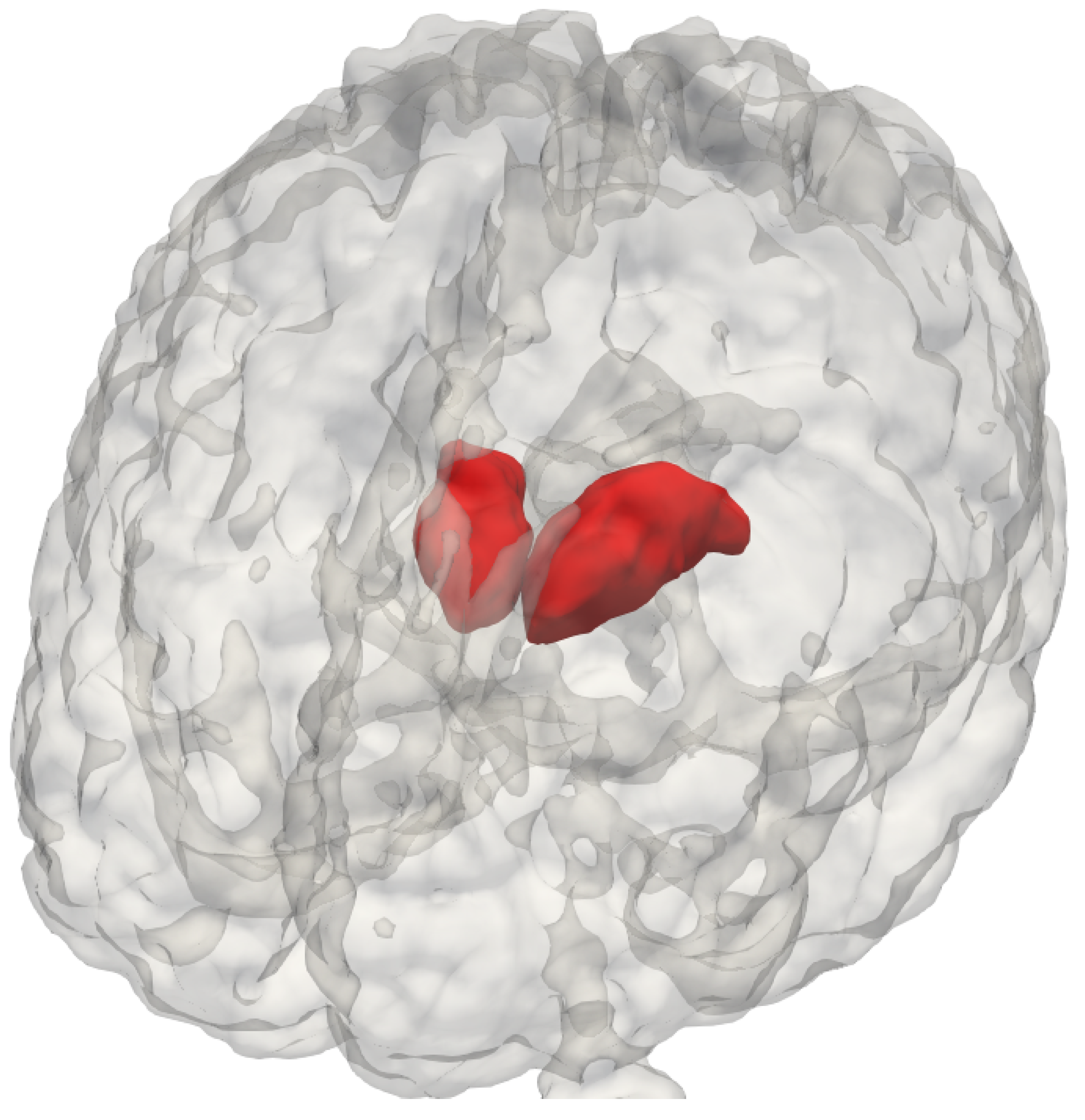
The thalamus (
Figure 1) is a bilateral subcortical brain structure. Each of its two parts measure on average 20 mm in the left–right direction (radiological convention) and 30 mm in the anterior–posterior direction [
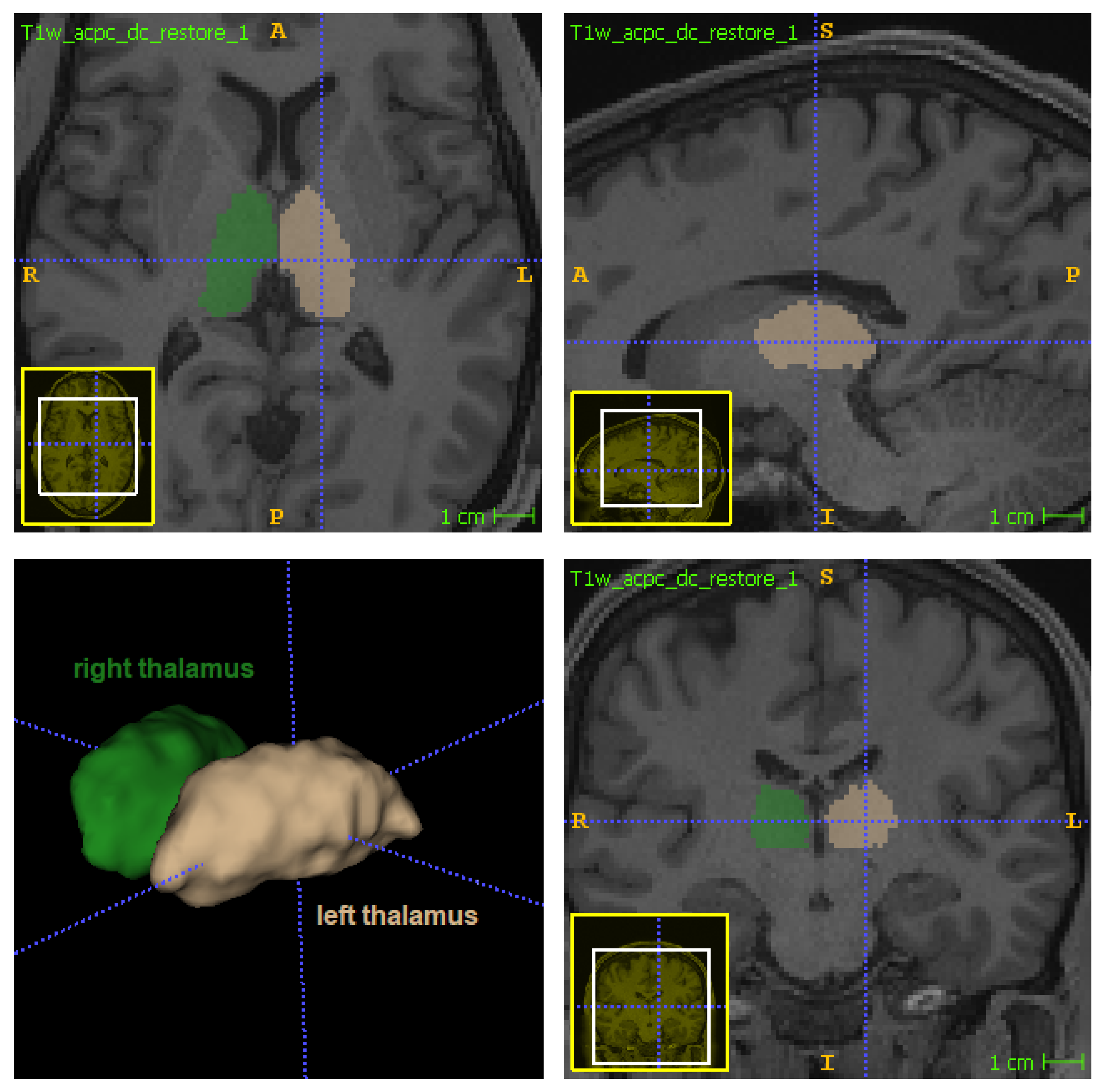
1]. It is located in the central region of the brain, below the ventricles and fornix, and above the hypothalamus (
Figure 1 and
Figure 2). Despite its relatively small volume, the thalamus can be further divided into nuclei depending on the cytological differences existing across different regions of the same structure [
1]. The thalamus also has a central physiological role in the nervous system, functioning as a signal transponder owing to the white matter connecting it to a wide area of the cortex. Furthermore, it is involved in other functions, including the regulation of sleep, alertness, motor functions, and spoken language [
1,
2].
Many neurological disorders are associated with thalamic changes. This region of the brain includes targets for deep-brain stimulation and stereotactic ablation for the treatment of symptoms of conditions such as Parkinson’s disease, essential tremors, epilepsy, chronic pain syndrome, and multiple sclerosis [
3,
4]. In the context of surgical planning, accurate segmentation is essential for the success of therapy. Relevant surgical approaches include focused ultrasound thalamotomy, where the segmentation requirement is the rapidity of its estimation for improving operation efficacy [
5]. Accurate segmentation is also highly desirable in the follow-ups and studies of the as-of-yet unclear mechanisms driving these diseases [
6].
Magnetic resonance imaging (MRI) is frequently employed to visualize the thalamus, as it enables the non-invasive observation of in vivo deep brain structures under safe conditions for the patient. A wide variety of automated tools are available for MRI-based thalamus segmentation. Nonetheless, manual segmentation is still considered the “gold standard”, as it overcomes the low contrast and resolution achievable in standard 1.5 and 3T T1-weighted acquisitions [
7]. In fact, these limitations in contrast and resolution may constitute a bias, thereby yielding suboptimal segmentation results. Unfortunately, manual segmentation has its own limitations: discrepancies owing to the scarcity of protocols [
8,
9,
10]; the need for trained raters; and an excessively large execution time [
7], especially for larger datasets. Consequently, the development of faster and more robust automatic thalamus-segmentation methods is crucial.
The T1-weighted scan is one of the most widespread MRI sequences owing to the rapidity and relative simplicity of its acquisition, visual similarity with anatomical slices, and good spatial resolution [
11,
12]. For these reasons, it is also one of the most used MRI types with both manual and automated segmentation methods. In the field of neurological structures, existing automated segmentation methods can be primarily categorized as atlas-based or deep-learning-based.
As atlas-based methods, the
fsl_anat [
13] tool of the FSL software and FreeSurfer [
14] represent atlas-guided thalamus segmentation approaches, serving as the most popular automated tools, despite their time-intensive underlying algorithms [
15] and tendency to overestimate the thalamic shape compared to manual segmentation [
7]. Recently, a less common structural acquisition of white-matter-nulled MP-RAGE images has been employed to collect data using a 7T MRI scanner, leading to the development of Thalamus-Optimized Multi-Atlas Segmentation (THOMAS) [
1]. Theoretically, such a sequence would enhance the thalamic contrast on a 7T MRI scanner. THOMAS has been successfully used to segment 12 thalamic nuclei with Dice coefficients of 0.85 and 0.7 for large and small nuclei, respectively. Unfortunately, only qualitative results were produced for its feasibility on 3T MRI, whereas quantitative validation is necessary given the known complexity of the task [
4,
16].
Methods built upon deep learning strategies allow for fast thalamic segmentation, at the cost of requiring a large quantity of data for training in order to avoid overfitting [
17,
18]. Some exceptional methods [
6,
19,
20] can obtain good segmentation results even with smaller datasets by using artifices such as multi-scale patches. However, generalizability cannot be ensured given an insufficient test set.
One of the most recent and high-performing deep learning techniques is QuickNAT [
17], which employs a Bayesian fully-convolutional neural network to estimate the thalamus shape from T1-weighted MR images, requiring only 20 s when using a GPU. This method uses multiple large datasets to ensure consistency across different MRI data.
The advantages derived from multimodality warrant further investigation. Indeed, the multimodality of MRI has enabled highly accurate performance, reaching Dice coefficients of 0.878 and 0.890 for the two thalami when calculated against manual segmentation [
21]. Specifically, the random forest algorithm was employed to generate predictions based on structural (T1 and T2-weighted) and diffusion-weighted MRI. In particular, diffusion MRI (dMRI) alone has been frequently employed in prior studies to perform this task [
21,
22,
23].
Among the most recently proposed works, Battistella et al. [
24] took advantage of the orientation-distribution functions calculated using the spherical harmonic model to detect and characterize the thalamus with satisfactory performance. In fact, the inherent cytological differences within the thalamus serve as the basis for the hypothesis of dMRI’s sensitivity to the microstructural modulations of this structure. By relying on the Fourier transform that relates the dMRI signal to the propagator from which the orientation-distribution function is calculated, information regarding the brain tissue architecture can be inferred for each voxel [
25]. This is possible because the propagator represents the probability that the water volume inside the brain undergoes displacement
r in diffusion time
, which reflects the diffusion process constrained by the walls of the compartment therein (e.g., the white matter axon). The use of dMRI to obtain microstructural details of brain tissue offers the potential to enable more robust and accurate segmentation procedures.
Despite the significant potential of deep learning methods and the use of diffusion data for thalamus segmentation, few attempts have been made to combine the two approaches for that purpose [
26,
27]. One reason behind the scarcity of research pertaining to this subject is the complexity of using multimodality on CNNs, specifically with dMRI. Additional steps demanded by the use of dMRI data with CNNs include: fitting a diffusion model and computation of diffusion tensor maps; complex registration processes among different MRI sequences; changes in the CNN architecture to handle multiple inputs; manipulation of diffusion tensor maps. All of these steps require a rigorous methodology to express the advantages of diffusion data. Additional challenges, such as the scarcity of large datasets and ground truth (manually annotated segmentations), are more pronounced in dMRI, as the acquisition is more costly and the interpretation of diffusion data is not as trivial as it is on T1-weighted images [
28].
The primary objectives of this study were to provide a benchmark for the development of more precise thalamus-segmentation methods, taking advantage of diffusion MRI data; promote fair comparisons among different methods; and interpret the contribution of dMRI to the segmentation task. The main contributions of this work are: a large processed benchmark dataset composed of annotated co-registered T1-weighted and diffusion MRI; a set of different thalamic masks for each subject computed using atlas- and CNN-based methods and statistically-combined masks; manual ground-truth data provided by experts; a baseline framework useful in the processing of diffusion data and additional training of CNNs for thalamus segmentation; and an ablation study on the contribution of dMRI to this task.
Motivation
As mentioned previously, the vast majority of thalamus-segmentation methods use exclusively T1-weighted images [
6,
15,
16,
17,
18,
19,
20,
29], an MR sequence that fails to present a good contrast on the thalamus borders (
Figure 3-T1). In contrast, diffusion MRI naturally accounts for the different properties of the brain’s microstructure [
28,
30,
31,
32,
33], leading to higher contrast for certain sub-cortical structures, and consequently greater potential as a tool for segmentation problems.
For example, when visualizing scalar maps computed from diffusion tensor imaging (
Figure 3), the frontiers of the thalamus with other structures are clearly visible: on FA maps, for instance, the boundary between the thalamus and internal capsule is shown with a higher contrast due to the differing anisotropic diffusivity of these structures.
Another indicator of the potential of dMRI for thalamus segmentation is the use of diffusion indices to parcel the thalamus [
2,
24,
34]. In summary, the parcellation of thalamic nuclei is reliable only when using diffusion MRI.
Considering that dMRI can highlight more differences between the thalamus and its neighboring structures than other MRI contrasts, it may even lead to a more appropriate delineation of the actual structure, thereby pushing the theoretical limits of segmentation performance for both manual and automatic methods.
Despite being able to carry a higher contrast for certain brain structures, dMRI presents some disadvantages, including: an excessive acquisition time in the MR scanner; typically lower spatial resolution compared to T1-weighted images; a high computational complexity owing to multiple diffusion directions; complex registration in cases where T1-weighted images or T1-derived annotations are needed simultaneously; and extra non-trivial processing steps [
31,
32], as in the cases of geometrical corrections and model fitting.
One of the primary motivations for the use of CNNs is a significant decrease in prediction time compared to other available methods. For instance, the segmentation of a whole brain can be achieved in a matter of seconds—i.e., QuickNAT requires 20 s when using a GPU—whereas atlas-based methods usually demand hours. Furthermore, the latest CNN methods represent the current state-of-the-art in terms of overlap metrics for segmenting brain structures [
17,
35].
The main downside of these approaches is the requirement for sufficiently large annotated datasets. Furthermore, the performance of these methods is closely linked to the quality of the data labels [
36]. In addition, the input data must be diverse and consistent to ensure satisfactory CNN performance. Specifically, the data and labels require appropriate standardization, especially when working with multimodal data [
37].
Despite the high performance of segmentation methods using T1-weighted images, prior studies have demonstrated the great potential of dMRI for improving the quality of thalamic segmentation [
2,
24,
26,
34]. However, preparing the dMRI to be used in conjunction with CNNs for this purpose is not a trivial task. Accordingly, a primary motivation of this work is the need for an appropriate dMRI processing pipeline for CNN approaches, and there are the additional objectives of providing the preprocessing methodology, preprocessed data, and a benchmark test set to facilitate comparisons with future works.
2. Materials and Methods
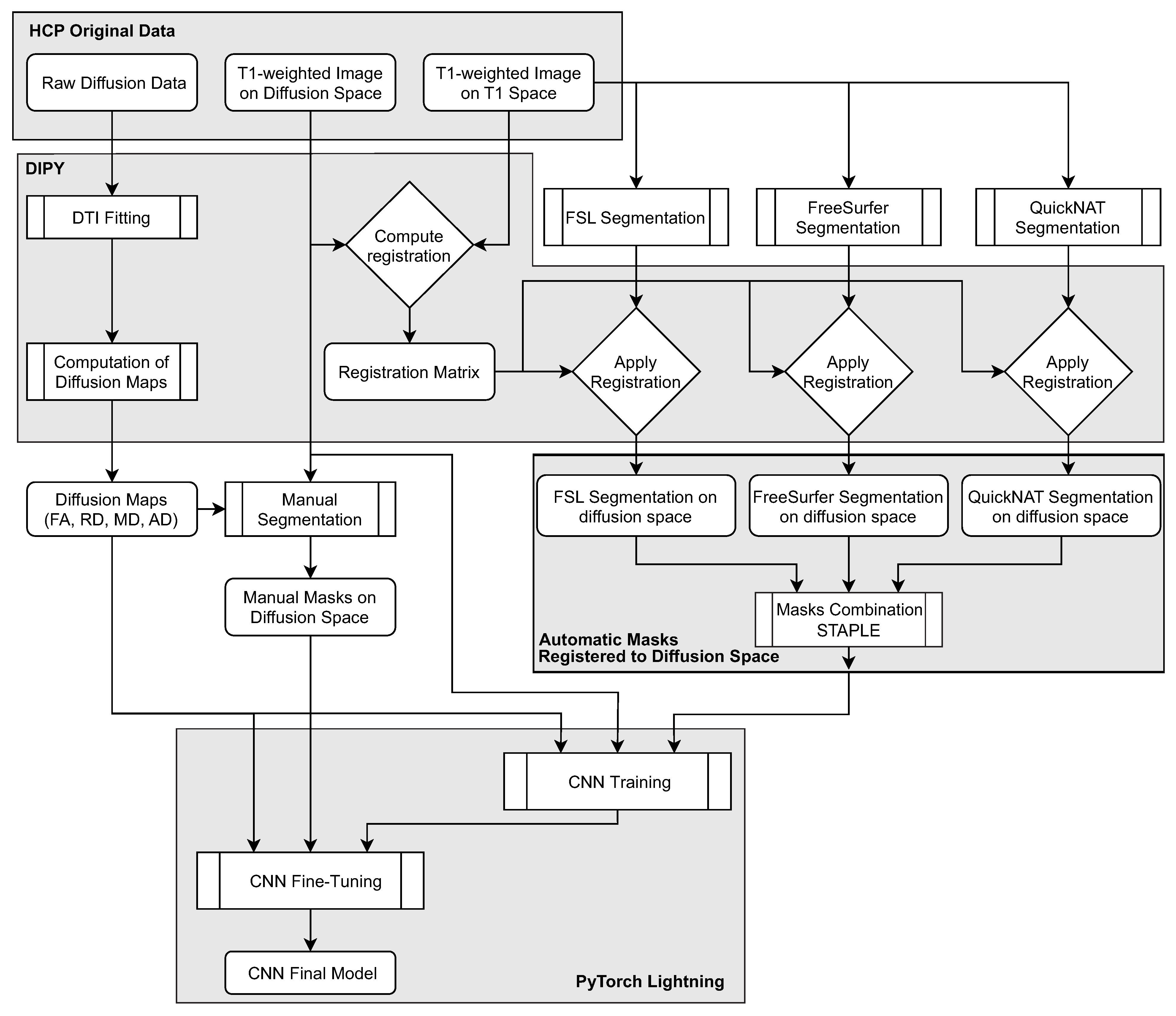
The following subsections provide details pertaining to the method’s pipeline (
Figure 4), including the preprocessing and organizational stages and the segmentation methods and CNN framework.
2.1. Dataset
The Human Connectome Project (HCP) [
38] is a consortium that studies brain connectivity in healthy adults and releases all relevant data. It provides MR images collected in many modalities, including the structural T1 and diffusion-weighted images employed throughout this study. HCP T1-weighted acquisition was performed using a 3D magnetization-prepared rapid acquisition gradient echo (MPRAGE) sequence (repetition time (TR)/echo time (TE) = 2400/2.14 ms, flip angle (FA) = 8
, field of view (FOV) = 224 mm, 0.7 mm isotropic resolution, 256 slices), whereas the diffusion-weighted images were acquired using a Stejskal–Tanner monopolar diffusion-encoding scheme (TR/TE = 5500/89 ms, FA = 160
, FOV = 210 mm, 1.25 mm isotropic resolution, 111 slices, b-values = 1000/2000/3000 s/mm
with 90 non-collinear gradient directions for each b-value and 18 b0 volumes) [
38]. The consortium provides minimally pre-processed data for both modalities [
39]. T1-weighted MRI data were corrected for gradient, readout, and bias field distortions, whereas dMRI data includes b0 intensity normalization and correction for susceptibility-induced b0 fields, eddy current, subject motion, and gradient distortions.
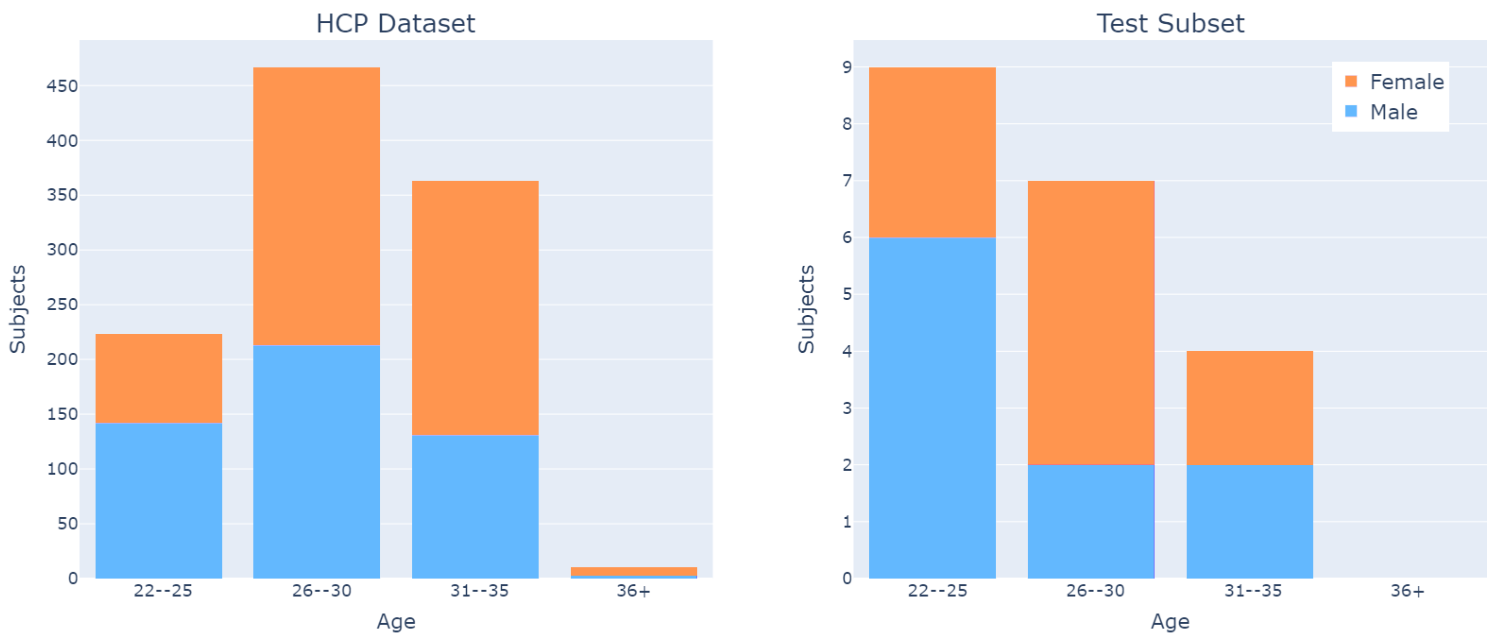
Although the HCP dataset encompasses data from more than 1200 subjects, a total of 1065 subjects had scans for both diffusion- and T1-weighted MRI. As 2 subjects were discarded due to issues with the registration process, the dataset used throughout this study includes 1063 subjects.
The dataset is fairly balanced with respect to subjects’ sex, and has an age distribution from 22 to 35 years (
Figure 5).
2.2. Silver Standard Creation
Since the use of manually annotated masks (ground truth) is impractical for a large dataset, a silver standard may be employed instead. The silver standard is a non-ideal mask, generated by automatic or semi-automatic methods, that may substitute the gold standard for specific purposes, as in the case of CNN training prior to fine-tuning.
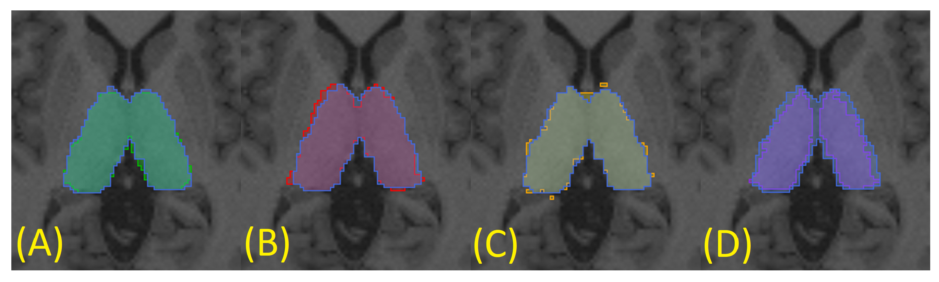
To generate a silver standard for each subject, three automatic segmentations were obtained through three different algorithms: FreeSurfer [
14] (
Figure 6A),
fsl_anat [
13] (
Figure 6B), and QuickNAT (
Figure 6C). This was achieved using only T1-weighted images (in T1 space), as the methods are optimized to work with this specific MRI sequence. Finally, the silver standard was generated using the STAPLE method [
40,
41] to statistically combine the three segmentations (
Figure 6). This procedure was performed for all subjects in the dataset.
2.3. Manual Segmentation
All manual segmentations were generated following the protocol described in the
supplementary material, which uses the T1-weighted images and diffusion tensor maps simultaneously, thereby circumventing the low contrast limitation and achieving a more reliable segmentation of the thalamus.
In summary, the thalamus manual segmentation protocol employed in this work considers the T1-weighted image and diffusion tensor maps, and the three views (axial, coronal, and sagittal), to facilitate specialized decision-making processes. It also used the ITK-SNAP software [
42] to simultaneously display multiple grayscale images (e.g., T1-weighted and FA) along with the segmentation.
The proposed manual segmentation protocol was designed to facilitate the task and stabilize the segmentation considering the relatively high inter- and intra-rater variability in thalamic manual segmentation for T1 images alone, as demonstrated in [
7]. Results of the proposed manual segmentation protocol are not intended to differ from the segmentation in T1, as they refer to the same structure.
Of the 60 subjects examined in the manual segmentation task, 16 were classified by a non-expert rater, and the remaining 44 by a physician with 15 years of experience in brain structure and manual segmentation on MRI. All manual segmentations performed by the non-expert also followed protocol and were used only to fine-tune the CNN. Only manual segmentations were considered for model evaluation, with a total of 20 subjects.
To evaluate the variability of segmentation between the expert and non-expert raters, five additional subjects were segmented by the latter, and certain metrics were computed (
Section 2.7). The comparison (
Table 1) indicates that the manual segmentations from the two raters are closer to each other than to the proposed silver standard, especially when considering the overlap (Dice coefficient) and volumetric similarity.
2.4. Data Processing
The HCP dataset was processed to ensure its compatibility with CNN training. Specifically, minimal steps were taken to standardize and organize the data for use. The processed benchmark dataset was subsequently released for public access.
Indices describing the brain microstructure were derived from the dMRI data by reconstructing signals using a diffusion tensor imaging (DTI) model [
43]. These models are frequently employed in clinical activity under the assumption that each diffusion signal coming from the brain tissue can be described by a Gaussian function. The dMRI signal fitting is therefore obtained by calculating the tensor, a symmetric 3 × 3 matrix whose parameters can be derived from the MR volumes acquired in different gradient directions. Such a tensor is a representation of the 3D diffusion process for any voxel of the 3D volume, and can be expressed via eigenvalue and eigenvector formulation.
The microstructural indices [
44,
45] used throughout this study were computed from such eigenvalues. These indices were: axial diffusivity (AD), radial diffusivity (RD), mean diffusivity (MD), and fractional anisotropy (FA). All relevant computations were performed using the DIPY library [
46] with the weighted least squares method. Only those dMRI volume images corresponding to a b-value of 1000 s/mm
(single shell DTI model) were selected. This process generated four 3D volumes, one for each microstructural index, for all subjects of the cohort.
Another crucial process applied to the data is the registration, which placed the diffusion- and T1-weighted images, and the masks, within a single space, allowing them to be simultaneously used by the CNN.
Although the HCP dataset comes with a T1w image registered to a diffusion space, it does not provide an appropriate affine matrix. Therefore, we computed the registration matrix (rigid transformation) using the T1w images on the T1 and diffusion spaces. Subsequently, the matrix was used to translate the masks to the diffusion space. It is important to emphasize that the registration was visually inspected in 20% of the dataset, including all subjects with manual segmentation. Likewise, all registration logs were inspected; the two discarded subjects were flagged.
The decision to transport the T1-weighted images to the diffusion space, rather than the other way around, was made because the scalar T1-weighted images do not suffer as much from voxel interpolation during the registration process as tensor images would. Since the masks are integer values representing structures of the brain, they were interpolated with the nearest-neighbor technique.
2.5. Data Organization
From the 1065 subjects selected for the dataset, the registration algorithm could not converge for 2 subjects, which were discarded. Subsequently, 963 subjects containing only silver-standard masks were allocated to the training set. From the remaining 100 subjects, 60 were manually segmented and used for fine-tuning and testing. A set composed of 40 subjects was reserved to increase the test set in the future (
Table 2).
All subject recruitment procedures and informed consent forms, including consent to share de-identified data, were approved by the Washington University Institutional Review Board (IRB) [
47]. Permission for using open-access data in the present study was obtained from the HCP.
2.6. Segmentation Method
Despite frequent proposals of newer architectures and frameworks, current state-of-the-art deep-learning-based methods, including QuickNAT [
17] and nnU-Net [
35], are based on the U-Net architecture, one of the most popular CNN architectures for medical imaging. We also employed the U-Net [
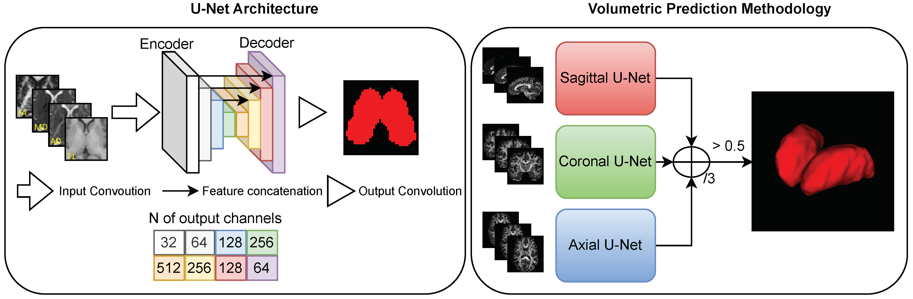
48] architecture to segment the thalamus, as it represents a baseline segmentation result for the proposed benchmark.
To segment the thalamus using a multimodality dataset, the U-Net model was trained with a multichannel input: each channel received T1w or diffusion images (
Figure 7). This is the standard U-Net architecture, which is able to handle any amount of input channels by changing the corresponding hyperparameter [
49,
50,
51,
52,
53]. When using more than one channel, the U-Net fuses all input channels in the first convolutional layer, transferring features extracted from all inputs to the inner layers.
We used image patches throughout the training and fine-tuning procedures, as U-Net is a fully-convolutional neural network (FCNN) [
54], whose training and prediction phases do not require images of the same size. This is advantageous for many reasons: it increases the amount of training data; it makes the model more immune to location variance, as the thalamus may be present anywhere within a patch; it balances the amounts of background and foreground present during training; and it simplifies the extraction of 2D images from the 3D MRI to feed the 2D CNN architecture.
For the output, we employed a softmax activation with two channels for the background and thalamus (foreground), respectively. The target for the output was the thalamus segmentation mask, guided by a soft Dice loss [
55]. During fine-tuning, we exploited the encoder-decoder nature of the U-Net, freezing the pre-trained encoder and updating only the decoder weights.
The aforementioned training strategy can be applied to multiple models. We used a multi-view 2D approach to obtain a volumetric thalamus segmentation (
Figure 7). First, we predicted the volumetric segmentation three times using different 2D CNN models trained for each respective slicing orientation (axial, sagittal, and coronal). Subsequently, the three volumetric predictions were combined into a single final prediction volume as follows:
. Here,
A,
S, and
C denote the activations for the axial, sagittal, and coronal networks, respectively. Although such a view aggregation requires more computation than a single-view 2D CNN, it significantly improves segmentation quality, primarily by eliminating low-confidence misclassified voxels from the predictions [
56]. Furthermore, it requires considerably less computational resources than an equivalent 3D approach. The latter does not guarantee superior performance to the single-view 2D approach [
57]. In fact, prior studies have shown equivalent results when comparing 2D view aggregation with the 3D convolutional approach [
17,
52,
58,
59].
2.7. Evaluating Metrics
The following metrics were used to evaluate segmentation performance on the test set, with the manual segmentation done by a specialist used as ground truth: Dice coefficient, false negative error, false positive error, Jaccard coefficient, and average Hausdorff distance. However, we focused solely on the Dice coefficient and average Hausdorff distance, as they will be used for the purpose of an open benchmark.
The requirement for different metrics to evaluate segmentation results arises from the complementarity of these metrics in comparing method output to the ground truth. For example, whereas the Dice coefficient evaluates the overall accordance between two objects, the average Hausdorff distance indicates the behavior of agreement in the shells of the volumes [
60].
To define some of the metrics used in this study, we consider the four basic cardinalities of the confusion matrix that indicate overlap between the two masks. True positives (TP): number of positive voxels included in both the automatic segmentation and ground-truth mask; false positives (FP): number of positive voxels included in the automatic segmentation but not in the ground-truth mask; true negatives (TN): number of voxels taken as negative (background) in both the automatic segmentation and ground-truth mask; false negatives (FN): number of positive voxels in the ground-truth mask that were not included in the automatic segmentation.
The
Dice similarity coefficient, or
Dice coefficient (
DC), is a spatial overlap index that ranges from 0 to 1, denoting zero overlap and complete overlap, respectively, [
61].
The
Hausdorff distance (
HD) is a measure of dissimilarity comparing image segmentations [
62]. Given the set of voxels
of mask
A and the set of voxels
of mask
B the
Hausdorff distance is such that
where
is the directed Hausdorff distance given by
where
is an arbitrary norm (in our case, Euclidean distance). In this work, the dimension of the Hausdorff distance is expressed in voxel size.
The
average Hausdorff distance (
AHD), or simply
average distance, is more stable and less sensitive to outliers than the conventional
HD, representing the mean
HD over all points
2.8. Computational Framework
To conduct the training process, we employed Python Jupyter Notebooks and PyTorch Lightning, a wrapper of the PyTorch library that facilitates the “software engineering” stages of the training process—e.g., logging, data loading, model checkpointing, and the training loop. Training was performed on an Nvidia RTX 2080 Ti GPU (11 GB GDDR6 and 4352 CUDA cores), i9-9900K CPU @ 3.60 GHz, and 64 GB of RAM.
With this setup, the training and fine-tuning, described in
Section 2.6 and
Section 3.3, require for each CNN model about 60 min and 15 min, respectively. The segmentation prediction for each CNN model takes less than 5 s. Among all processes described in this work, only training, fine-tuning, and prediction ran on the GPU, as they are the only ones designed to use CUDA cores.
2.9. Leaderboard Platform
For the benchmark, we are hosting a competition on the CodaLab platform [
63], where participants may submit their segmented data to be automatically evaluated and entered in the leaderboard. Our competition can be found at
https://codalab.lisn.upsaclay.fr/competitions/8329 (accessed on 20 April 2023).
The evaluation criteria are based on the Dice coefficient score, computed using the complete testing dataset. Individuals and groups can submit their segmented data directly on the platform, with a limitation of two submissions per day. To appropriately submit segmented data, detailed information can be found on our CodaLab page.
3. Experiments and Results
The following subsections present the experiments conducted throughout this study, and their results.
3.1. Data Preparation for CNN Training and Predicting
The first step encompasses the filtering and normalization of data. The T1-weighted MR, AD, RD, MD, and FA images were all normalized between zero and one to be used as input for the CNN. Prior to that, a percentile filter was applied to eliminate 0.2% of the highest values in each channel, as defined in preliminary experiments. This step is necessary to eliminate any spurious voxel values and keep all input channels within the same normalized range. Failure to follow this step may result in suboptimal performance, as high-value voxels and discrepancies among the maximum values of each map may obscure brain tissue information from the CNN, and any comparison study would not be valid.
The next step is to generate patches from the images to be used for training. Patches were extracted for the three data views, allowing three corresponding models to be trained and combined. Of the 60 patches extracted for each subject, all were randomly selected; however, 50 were centered inside the thalamus to ensure good balancing of the amounts of voxels inside and outside the segmenting structure. We stress that all input channels and masks must be taken to have exactly the same size and coordinates for each patch to maintain the alignment of input data.
Data were subsequently allocated among training, validation, fine-tuning, and testing subsets. The testing set comprised the data of 20 subjects, for whom manual segmentation was performed by the specialist. For the training phase, 963 subjects (
Table 2) were split among the training and validation sets according to an 80:20 ratio.
A data augmentation method was also applied during model training. This augmentation was not performed on the raw diffusion or tensorial data, but on the scalar maps computed from the DTI models, as the interpolation of tensors is not as straightforward as that of scalar maps. Two data augmentation techniques were applied to the images: rotation constrained by limits of to with a random distribution, and horizontal reflection. We note that the latter does not apply to the sagittal view, which does not exhibit lateral symmetry. Furthermore, the masks and input channels must undergo identical transformations to keep them aligned. Data augmentations such as translations were not used, as the patching also functions as an augmentation method to make the CNN more generalizable to translations.
Finally, the training masks were appropriately standardized, as the automated segmentation methods (FSL, FreeSurfer, QuickNAT, and STAPLE) assign different labels to each thalamus with respect to laterality. The standardization consists of setting the background and structures to zero and one, respectively, (we employed a single label for both thalami). Nonetheless, the offered framework supports multiple labels, allowing for multi-structure segmentation as necessary.
3.2. Setting Hyperparameters
The hyperparameters for the training were obtained from preliminary experiments. Patch sizes of 64 × 64 were chosen based on the optimal balance, training time, and data storage. The learning rate was defined as
, with a decay factor of
for every time the validation loss function did not yield a significant improvement for 20 epochs. We defined an offset of 30 epochs for training to terminate in the absence of improvement. Adam was selected as the optimizer, as it yields substantially faster convergence and better quantitative results than SGD [
64].
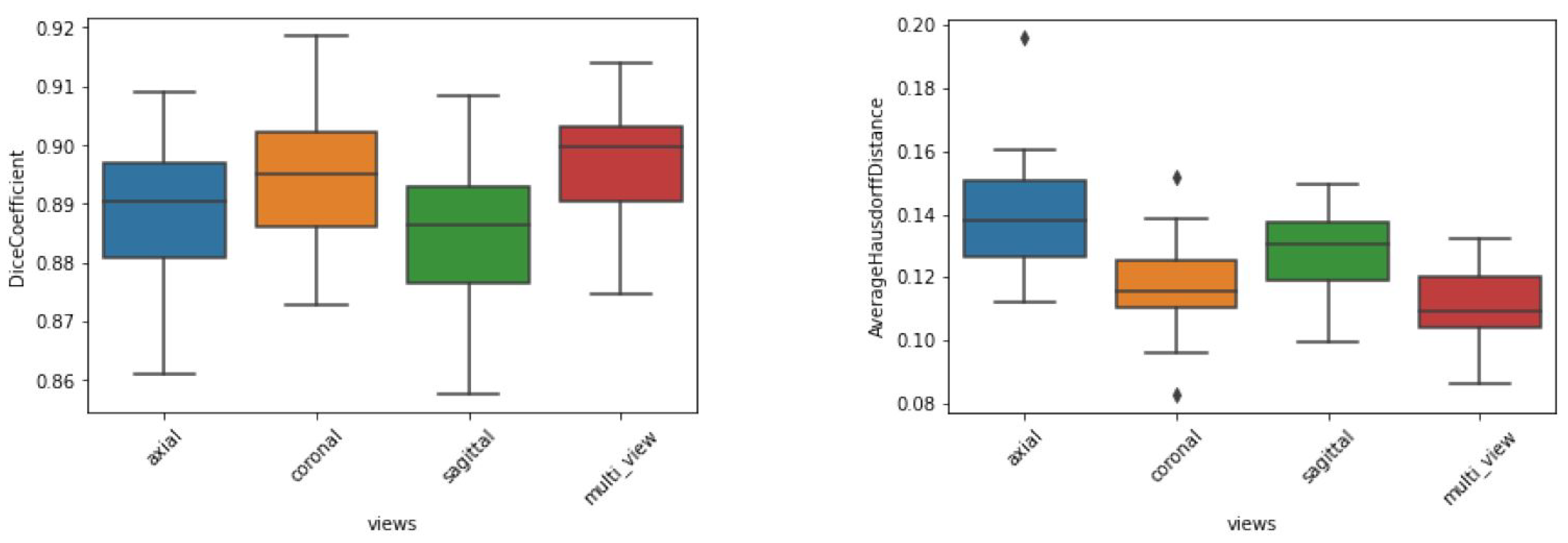
The preliminary experiments also helped to define the approach regarding single or multiple views. Using all available channels as input, the dice metrics of the test dataset (
Figure 8) indicate that the sagittal and axial views led to the worst results, whereas the coronal and combined views led to the best results. We also note that the aggregated view yielded the best AHD in terms of both average and standard deviation, indicating better and more stable segmentation behavior. This occurred because the aggregation of views corrects any misclassified voxels that appear far from the segmented thalamus. Accordingly, view aggregation was chosen as the approach to be used.
3.3. Gaining Performance by Fine-Tuning
As the silver-standard mask was computed by combining three other automatic segmentations, the CNNs were not initially fit to the manual segmentation protocol. Instead, the CNN models were replicating the segmentation resulted from the STAPLE method. To make the CNN model replicate the manual segmentation (ground truth), fine-tuning was conducted with manually annotated data, presenting a substantial improvement (
Table 3).
Fine-tuning was performed by freezing the encoder component of U-Net and training solely the decoder component. Conceptually, the feature extraction of the CNN model was kept intact, and the reconstruction of the segmentation was adjusted to the manual label. The same training hyper-parameters from the training phase were used during the fine-tuning phase.
During the fine-tuning phase, 40 subjects with manual segmentation as ground truth were used (
Table 2). The input configuration (input channels and their order) was kept identical.
3.4. Input Maps Ablation Study
As our primary hypothesis assumed that diffusion tensor maps can improve the quality of thalamus segmentation, the performances of models trained with each input map individually were compared to those of models trained with a combination of input maps. All models were trained using the data distribution described in
Section 3.1. The reported results are the average metrics among the 20 subjects from the test set.
The results (
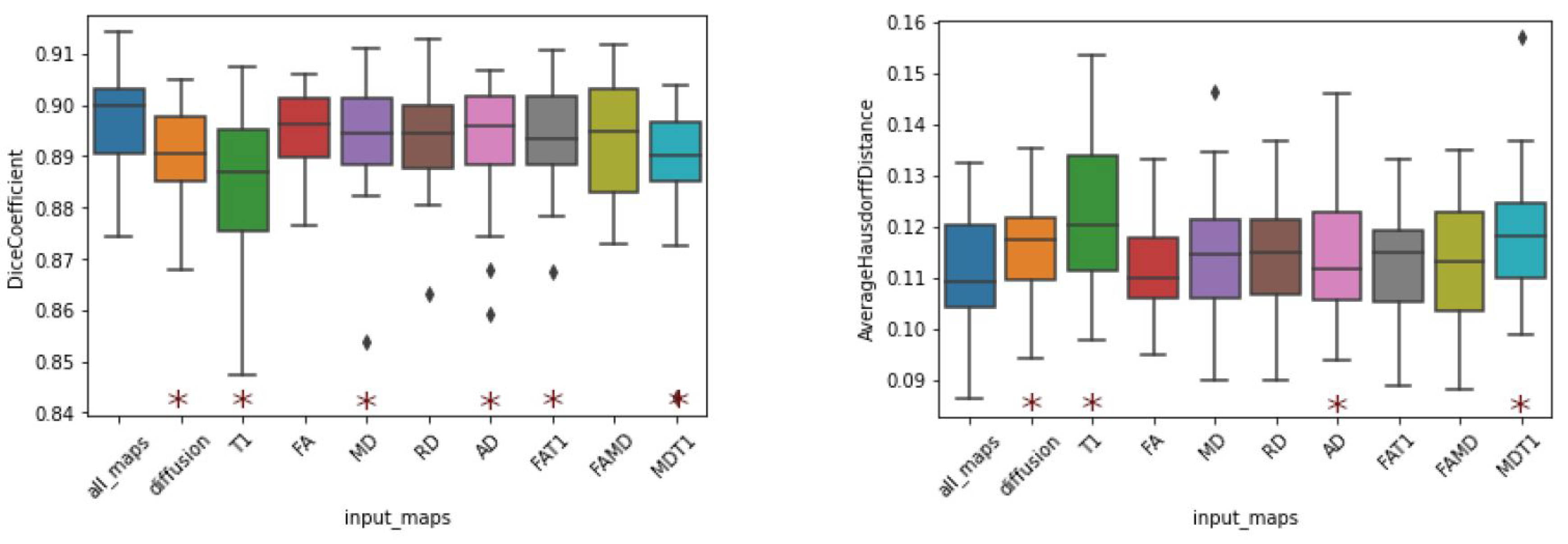
Table 4) indicate that the model trained on T1-weighted images yielded the worst results for every computed metric. While they are still within state-of-the-art levels, the worst Dice coefficients were obtained when the T1-weighted image was the only input channel (DC of 0.8837). The same consideration is valid for the average Hausdorff distance (AHD of 0.1230).
In contrast, models trained using diffusion tensor maps as input (single or combined maps) exhibited improvements in Dice score. In fact, the worst result presented by a model trained with a single diffusion map was a Dice coefficient of 0.8925 (AD), and the only combined-channel model that yielded a Dice coefficient below 0.89 was that trained on MD and T1. Furthermore, all combined models produced superior results to those of the model using solely T1 images.
Noteworthy results were also obtained by the model trained on the combination of all available maps. This combination, which can be regarded as the addition of T1 to the combination of all diffusion maps, improved the DC from 0.8904 to 0.8970. Nonetheless, if we consider the addition of diffusion indices to T1, the DC increases from 0.8837 to 0.8970, representing a much more substantial improvement. Regardless of interpretation, this combination yielded the best performance in terms of the evaluation metrics, indicating that the segmentation that uses all input channels exhibited more agreement with the ground truth. This result is intriguing, as T1 images were associated with decreased performance when combined with singular diffusion maps (FA and MD).
Furthermore, results regarding the standard deviation reflect the segmentation stability for each map and certain combinations (
Figure 9). Again, we note that models trained on T1-weighted images exhibited the highest dispersion in both DC and AHD. Nevertheless, among the models trained with a single input, that trained with FA, produced the best average and dispersion results.
A statistical analysis was conducted through a two-sided Wilcoxon signed-rank test to compare the CNN models (
Figure 9) and other methods (
Figure 10) in terms of performance against our best model, namely, the model that used all diffusion maps in conjunction with T1-w images as input. We note that in addition to exhibiting better metrics when compared to other methods, our approach’s results are significantly different, statistically. Identical analyses were performed to compare every CNN model with a single input channel (
Table 5) to interpret their equivalences. From these tests, it is apparent that the statistical differences between the T1 models and any of the diffusion models are much more significant than those between models that use diffusion maps as input. This implies that any of the tested CNN models that use diffusion maps as input produce different results when compared to a CNN with T1w images as input. Simultaneously, it is apparent that all CNN models using single diffusion maps as input produced mutually similar results.
3.5. Comparison with Existing Segmentation Tools
The results achieved by the proposed pipeline were compared to those of common methods. Tools that are easy to use and well-validated in the thalamus-segmentation task were selected for reproducibility purposes. To maximize diversity and generalizability, two classes of segmentation methods were employed: atlas-based and CNN-based.
This comparison may be considered somewhat biased, as the ground-truth was generated with a combination of T1-weighted images and dMRI, whereas all other methods only used T1. However, the masks generated with the assistance of dMRI are assumed to be equivalent to those generated only on T1, as both represent the same structure.
FSL and FreeSurfer were evaluated as representative atlas-based methods. Their segmentations were computed in the T1 original space, and subsequently registered to the diffusion space to be compared against manual segmentation.
The QuickNAT framework was evaluated as an off-the-shelf CNN-based method. Although the original QuickNAT weights were not fine-tuned to this specific dataset, all input data were normalized according to the author’s requirements (FreeSurfer’s mri_convert –conform command).
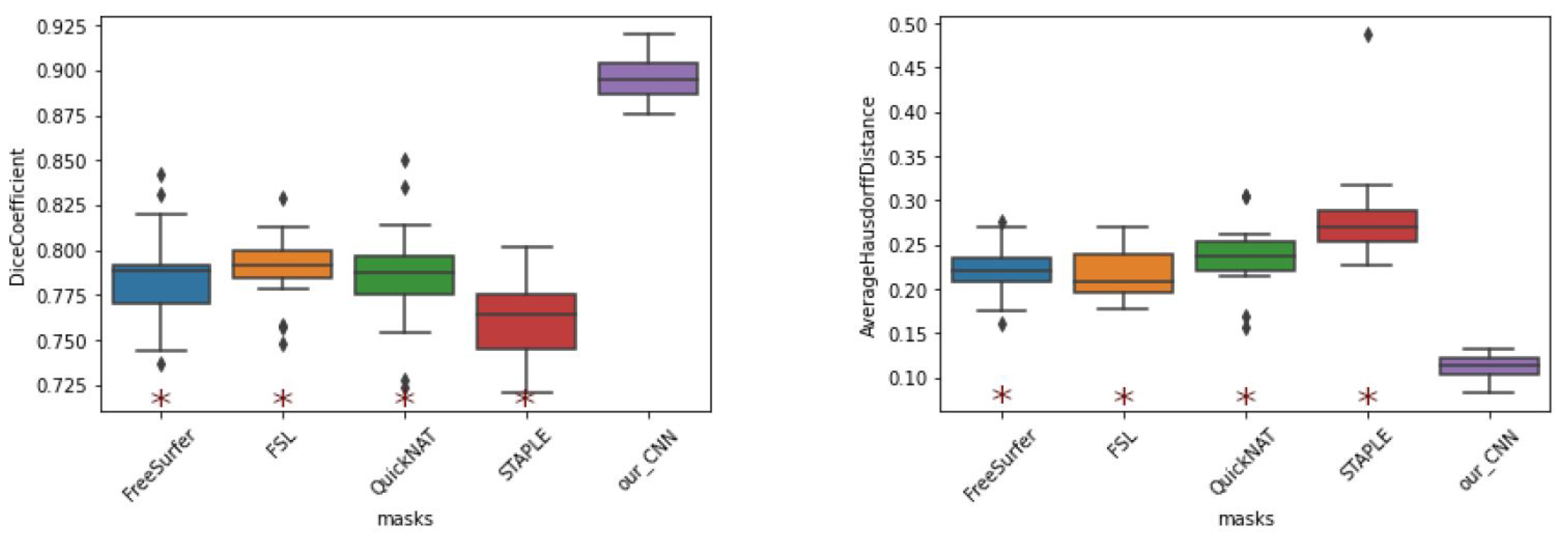
The results (
Figure 10) indicate that the best evaluating metrics, excluding those exhibited by our method, were obtained by FSL. All other methods, including STAPLE, exhibited considerable differences in performance compared to the proposed method. While these methods exhibited Dice coefficients in the range of 0.75 to 0.78, our CNN model achieved DC values exceeding 0.9.
3.6. Qualitative Results
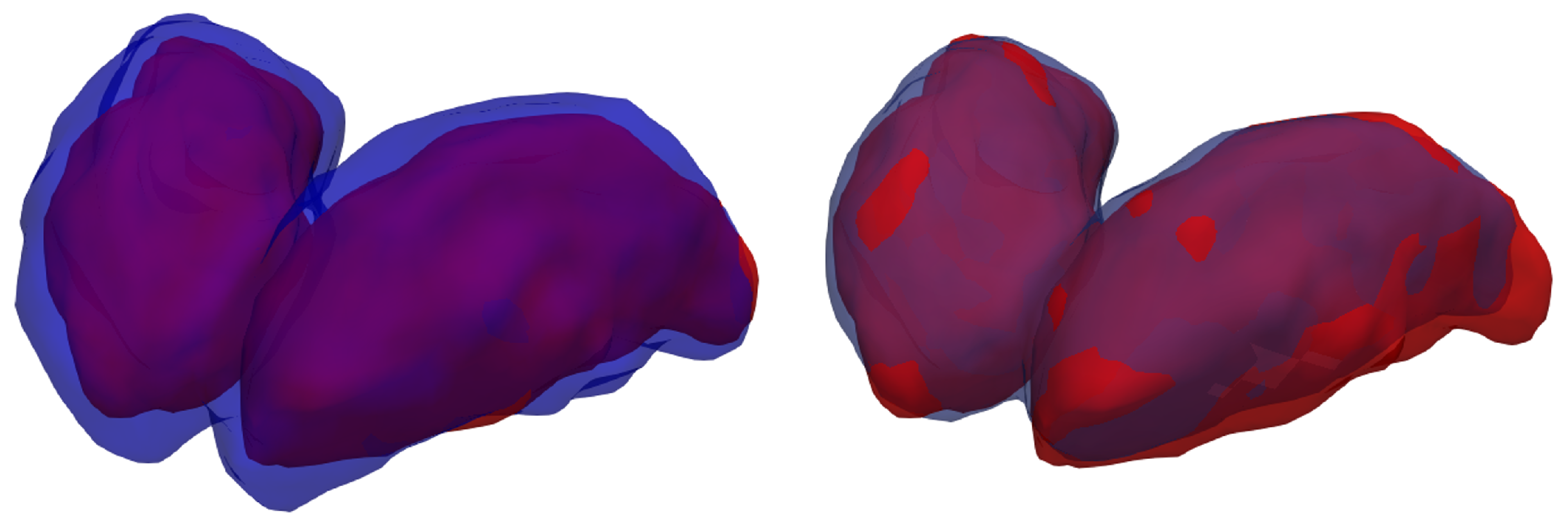
A visualization of the 3D segmentations is used to display the similarities and differences between the ground-truth and each method’s results (
Figure 11).
When comparing the manual annotation with the silver-standard mask, is is apparent that the latter considers the thalamus a much broader structure than the former. Other studies [
7] have observed similar results. Another important consideration is that the segmentation performed by the model after fine-tuning exhibits only minor differences when compared with the specialist’s annotation, with only a few voxels misclassified the borders of the thalami.
4. Discussion
Fine-tuning represents an effective approach when adjusting a model to manually segmented data. Prior to fine-tuning, our CNN models produced inferior results compared to those achieved by the atlas-based methods and QuickNAT segmentation. However, the fine-tuning process yielded an absolute improvement of approximately 0.12 in the Dice coefficient. It is important to remember that the encoder was frozen throughout the fine-tuning phase, and only the decoder weights that reconstructed the segmentation were trained.
Although minor differences in metrics were observed when aggregating all input, the diffusion indices computed from DTI clearly improved the quality of thalamus segmentation when used as input channels to the CNN. These differences in metrics were more significant for the FA map and combination of all available maps when compared to the case of using T1-weighted images alone as input. Further improvements may be obtained by extending the proposed approach to other microstructural indices [
65], especially when multi-shell data, such as NODDI and MAP-MRI, are available, as for HCP.
As a single-input channel, T1-weighted achieved a Dice coefficient of approximately 0.88, representing the current state-of-the-art in thalamus segmentation, as reported in the original QuickNAT work [
17]. Therefore, the proposed method surpasses state-of-the-art performance by incorporating dMRI, showing that aggregated multimodal information is beneficial for the thalamus-segmentation task.
The DC attained by our reproduction of the QuickNAT was in the range of 0.79, as opposed to the result of 0.88 reported by [
17]. However, we stress that the QuickNAT model was not fine-tuned to this specific dataset, and the only addition to the framework was the “FreeSurfer conform”, as it is a requirement for the QuickNAT pipeline.
Among the three possible views, the sagittal view yielded the lowest dice coefficient. A possible reason for this occurrence is the lack of thalamus symmetry under this view, which restricts the horizontal-reflection technique. Furthermore, the thalamus shape is more elongated in the anteroposterior axis, favoring the partial volume issue being more pronounced in this view. This also explains the best segmentation quality in the coronal view, where the thalamus exhibits the smallest cross section.
Our best results were obtained when using all input maps simultaneously (diffusion combined with T1). However, certain specific combinations unexpectedly led to deteriorated performance; i.e., the combination of the FA and MD yielded worse results than either of its constituent maps. We hypothesize that the aggregation of maps with small statistical differences is disadvantageous for the CNN model, as the resultant increase in information does not outweigh the increase in complexity. However, further investigation is required to understand this mechanism and determine the optimal map combinations for this task.
Although the FSL masks yield better validation metrics compared to other automatic masks, they were not selected as the silver standard during the training phase. Instead, the masks created by combining FSL, FreeSurfer, and QuickNAT via STAPLE were used for this purpose, as the combination of atlas- and CNN-based methods is more likely to eliminate model bias.
As all CNN models used and shared throughout this study were trained and evaluated on these specific benchmark data, we do not expect identical results if they are applied directly to other datasets. This is one of the limitations of the presented method. To successfully use our models and framework with other data, we recommended retraining or fine-tuning the models in the new data domain. With appropriate fine-tuning, the model is expected to yield comparable performance irrespective of dataset.
Additionally, our method was not tested on data from patients. Thus, in the presence of disease, the performance of the method cannot be ensured. Actually, the performance is expected to decrease if the model is not fine-tuned to adverse conditions.
The only segmented structure considered throughout this study was the thalamus. However, the framework proposed here also offers the possibility of working with other structures—such as the caudate, hippocampus, and putamen—as the dataset is published with a variety of pre-segmented structures.
Future work will focus on segmenting the thalamus nuclei. The presented framework is also able to perform structure parcellation—e.g., thalamus parcellation into nuclei—if the proper ground truth is available. For this purpose, other diffusion maps, such as the tensorial morphological gradient [
22], could be beneficial to achieving optimal results.
5. Conclusions
This study presents a ready-to-use framework for the development of thalamus-segmentation methods, comprising a processed multimodal dataset, code for reproducing the baseline model, and a test set for benchmarking. The dataset, based on the HCP data, encompasses a total of 1063 processed subjects with diffusion data, T1-weighted images, segmentation masks from FSL, FreeSurfer, QuickNAT, and a combination of the aforementioned masks through the STAPLE method. Furthermore, the dataset includes a subset with professionally segmented images.
For benchmarking purposes, researchers can submit their predictions to a leaderboard made available on our Codalab platform. A complete framework for training a CNN model is also available on our GitHub for other researchers to build upon.
Our proposed method combines T1-weighted images with diffusion MRI, representing a valid option for accurate segmentation of the thalamic structure. We demonstrated that the addition of diffusion MRI yields improvements in thalamus segmentation. Comparisons with existing state-of-the-art methods indicate the superiority of our approach, although a more fair comparison would demand the fine-tuning of QuickNAT using our manual masks.
The automatic generation of silver-standard masks circumvented the lack of a large volume of manually annotated data. The model, pre-trained on the silver-standard mask and fine-tuned on a small quantity of manual masks, led to an absolute improvement of 0.122 in the Dice coefficient.

 and
and 


