Multi-View Joint Learning and BEV Feature-Fusion Network for 3D Object Detection

Abstract

Traditional 3D object detectors use BEV (bird’s eye view) feature maps to generate 3D object proposals, but in a single BEV feature map, there are inevitably the problems of high compression and information loss. To solve this problem, we propose a multi-view joint learning and BEV feature-fusion network. In this network, we mainly propose two fusion modules: the multi-view feature-fusion module and the multi-BEV feature-fusion module. The multi-view feature fusion module performs joint learning from multiple views, fusing features learned from multiple views, and supplementing missing information in the BEV feature map. The multi-BEV feature-fusion module fuses BEV feature map outputs from different feature extractors to further enrich the feature information in the BEV feature map, in order to generate better quality 3D object proposals. We conducted experiments on a widely used KITTI dataset. The results show that our method has significantly improved the detection accuracy of the cyclist category.For cyclist detection tasks at the easy, moderate, and hard levels of the KITTI test dataset, our method improves by $1.57\%$, $2.03\%$, and $0.67\%$, respectively, compared to PV-RCNN.

1. Introduction

With developments in the field of automatic driving, the 2D object-detection network in the traditional image domain has increasingly failed to meet the safe driving requirements of autonomous vehicles in real-world scenes. When an autonomous vehicle drives in 3D space, it needs to recognize the 3D spatial information of obstacles to plan a safe path and avoid obstacles. Therefore, in the field of automatic driving, a powerful 3D object-detection network is needed to perceive and understand 3D scenes.

The point cloud obtained by Lidar contains spatial geometric information of objects, which can be used to measure the shape and position of objects in 3D space. Therefore, the 3D object-detection network [1,2] for Lidar point clouds is one of the most important research directions in this field. In general, 3D object detectors for Lidar are divided into single-stage detectors and two-stage detectors. The single-stage detector includes a preprocessing module, feature-extraction module, and detection head, while the two-stage detector includes an additional refinement module.

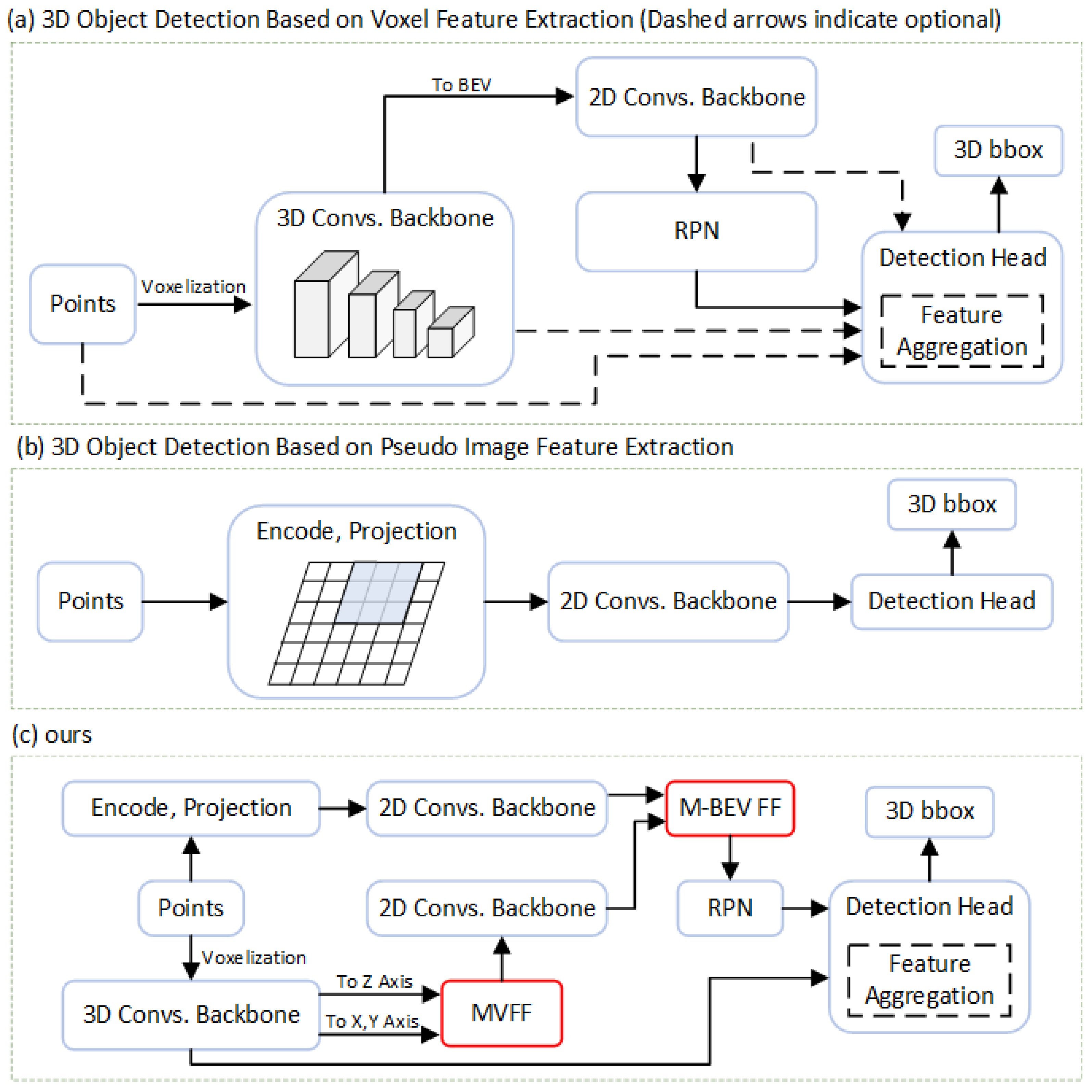
Lidar provides disordered point clouds. If we directly extract the features of the point clouds, numerous query operations will result, with low efficiency. Figure 1a,b show two commonly utilized methods for 3D object detection. In method (a) [3,4,5,6], first, the 3D space is discretized into voxels of the same size, and then the attributes of the points in each voxel are extracted as features of the voxel. At the voxel level, the 3D convolution operation is used to extract the features of the voxels. Second, the convolved voxel features are projected onto the 2D BEV input to the RPN (region proposal network) to predict the 3D region of interest (ROI). For a two-stage detector, the ROI is also refined in the detection head to achieve better 3D object-detection results. Method (b) [7,8,9] encodes the point cloud and directly projects it to obtain a BEV feature map. After feature extraction by the 2D backbone, the BEV feature map is input to the detection head to obtain detection results.

For certain reasons, most 3D object detection methods based on Lidar point clouds generate 3D object proposals using the 2D BEV feature map [10,11,12]. First, we can use or improve the mature 2D object-detection technology to extract the BEV feature map at a deeper level. Second, the projection of 3D objects (e.g., cars, pedestrians, and cyclists) is naturally separated in the BEV angle, and there is no serious occlusion problem. If we project in the X or Y direction, serious occlusion problems will occur in scenes with dense objects. Therefore, it is a good choice to use the 2D BEV feature map to predict 3D object proposals. Last, we perform similar operations without the occlusion problem in 3D space, but it requires considerable computation and time, and the inference efficiency is low.

The 2D BEV feature map occupies a key position in the entire 3D object detector, so the amount of information it contains will directly affect the prediction performance of the detector. The current popular 3D object detection methods [10,13] only use a single BEV feature map to predict 3D proposals. However, during the generation of BEV feature maps, voxel features are projected into the 2D plane, resulting in a significant reduction in the resolution of the z-axis and a compression of dimensions, which can lead to incomplete feature information in the 2D BEV feature map.

To solve the above problems and provide the missing information of the BEV feature map, as shown in Figure 1c, we propose a multi-view joint learning and BEV feature-fusion network that fuses the BEV feature map output from multiple modules to supplement the feature information of the BEV feature map. The enriched BEV features enable the RPN to predict high-quality 3D proposals, thereby improving network detection performance, especially for detection tasks with smaller targets such as cyclists and pedestrians. Our contributions are summarized as follows:

(1)

We propose a new multi-view joint learning and BEV feature-fusion network, which can overcome the information loss with a single view and enrich BEV features by adaptively fusing BEV feature maps.

(2)

We propose a new module in the voxel-based feature extraction branch that supplements the information lost in the BEV feature map due to the compression of the Z-axis resolution by projecting 3D features in the RV (range view) and SV (side view) and by incorporating them into the BEV feature map.

(3)

We compare the KITTI dataset with popular 3D object-detection methods. The results show that our network improves the detection performance of cyclist categories.

The remainder of this paper is structured as follows. We discuss the related work in Section 2, introduce our 3D object-detection network in Section 3, discuss our experimental results in Section 4, and summarize this paper in Section 5.

2. Related Work

In recent years, various 3D object-detection networks have been introduced. Generally, according to different feature extraction methods, existing networks are divided into the following categories: point-based methods, voxel-based methods, pseudo-image based methods, and hybrid methods.

Point-based 3D detection: A point cloud can directly represent the underlying spatial geometric information of an object and has the characteristics of sparsity, irregularity, and disorder. Therefore, in a point-based network, feature extractors need to be able to learn features from the original points. Because traditional feature extraction methods, such as CNN, cannot be directly used for irregular original point clouds, most point-based methods directly extract features point by point. PointRCNN [14] extracts features point by point, divides the point cloud into front attractions and background points, and then uses a bottom-up approach to generate high-quality 3D region recommendations for each front attraction. Point-GNN [15] directly uses a graph neural network on a point cloud to retain the irregularity of the point cloud and then extracts the point cloud features by iterating vertex features on the same graph. Point-based feature extractors can retain high-resolution 3D structure information, but point-by-point feature extraction will incur high computing and time costs. 3DSSD [16] proposes a lightweight single-stage target detector that uses a fusion sampling strategy to ensure sufficient internal points in the foreground instance, and then designs an anchor-free frame-prediction network to meet the requirements of high accuracy and speed.

Voxel-based 3D detection: Voxelization divides a point cloud into evenly spaced voxel grids, converts irregular shape data into regular shape data, and then uses traditional mature feature extractors to extract voxel features to complete 3D object-detection tasks. VoxelNet [17] uses the above idea to voxelize a point cloud and then uses a 3D CNN to extract the features of sparse voxel mesh to aggregate the spatial context information and obtain the expression of local geometric information of 3D objects. SECOND [12] introduces a sparse convolution method, which improves the speed and efficiency of feature extraction and enables finer voxel granularity when voxelizing point clouds. The voxel R-CNN [10] network fully utilizes voxel features and spatial context information and proposes a fast query technology in the ROI refinement stage to improve the accuracy and speed of 3D object detection. The SE-SSD [18] network adopts the idea of knowledge distillation, introduces the teacher–student model, and uses IoU-based matching strategies to filter soft objects from the teacher network and to encourage the student network to infer complete object shapes. AGO-Net [19] associates the perceptual features from point clouds with more complete features from conceptual models, enhancing the robustness of extracted features, especially for occluded and distant objects.

Pseudo-image-based 3D detection A pseudo image is obtained by sparsely and irregularly projecting onto a plane. Pseudo images are compact and orderly representations of point clouds, which have at least the following two advantages. First, pseudo images are 2D, and rich features can be extracted using mature, 2D feature extractors or backbone networks. Second, because pseudo images are obtained by point cloud projection, 3D spatial geometric information is retained to a certain extent, which is conducive to accurate position estimation. The PointPillars [9] network divides point cloud data into pillars along the X and Y axis (regardless of the Z axis direction), encodes the characteristics of the midpoint of the pillar and projects them onto the BEV to obtain a pseudo BEV image, and then uses a 2D CNN with high computational efficiency to replace the 3D CNN for end-to-end 3D object detection. The RangeDet [7] network projects the point cloud onto RV and introduces a meta-kernel convolution operation, which makes the convolution kernel weight depend on the geometric information of the convolution center point and neighborhood points and improves the detection accuracy of distant objects and pedestrians. The RangeRCNN [8] network uses the expansion convolution to extract features of RV images, uses the RV-PV (point view)-BEV module to convert features from RV to BEV, and then generates 3D proposals on BEV.

Hybrid 3D detection The hybrid method attempts to fuse the point-based method, voxel-based method, and pseudo-image-based method to achieve the purpose of complementation and then to obtain feature vectors containing rich information to improve the performance of the 3D object detector. The PV-RCNN [11] network uses PointNet++, sparse convolution and 2D convolution to extract original point features, voxel features, and BEV features, respectively, and then aggregates these features to a small number of key points sampled for refinement of 3D object recommendations in the second stage. The PV-RCNN++ [20] network improves the strategy of the original network sampling key points and the feature aggregation method, reduces the network computing cost and improves the running speed while ensuring the accuracy.Considering the sparsity of point clouds, deformable PV-RCNN [21] adds the idea of deformability to PV-RCNN, adaptively extracting features based on the density and object size of point clouds and improving the detection accuracy of small and distant targets. RSN [22] predicts the foreground spots from RV images, voxelizes the predicted foreground spots, and applies sparse convolution, which increases the efficiency of sparse convolution and object detection accuracy.

Among the above methods, most methods generate 3D object proposals using single-view feature maps, but there is a problem of information loss in single feature maps. Therefore, we propose the multi-view joint learning and BEV feature-fusion network to fuse the features of multiple feature maps for information compensation, thereby generating fused feature maps for predicting high-quality 3D object proposals.

3. Method

In this section, we introduce our 3D object-detection network, which is a two-stage 3D object-detection framework based on voxel and pseudo images.

The voxel-based two-stage 3D object-detection network generally uses the voxel CNN with sparse convolution [10,12] as the backbone of feature extraction, directly extracts 3D features, projects the features onto the BEV, predicts 3D ROI using the RPN, and refines the ROI in the detection head to obtain the detection results. The pseudo-image-based 3D object-detection [7,9] network uses sophisticated feature extractors to extract richer feature information, including 2D features and 3D features, for final result prediction.

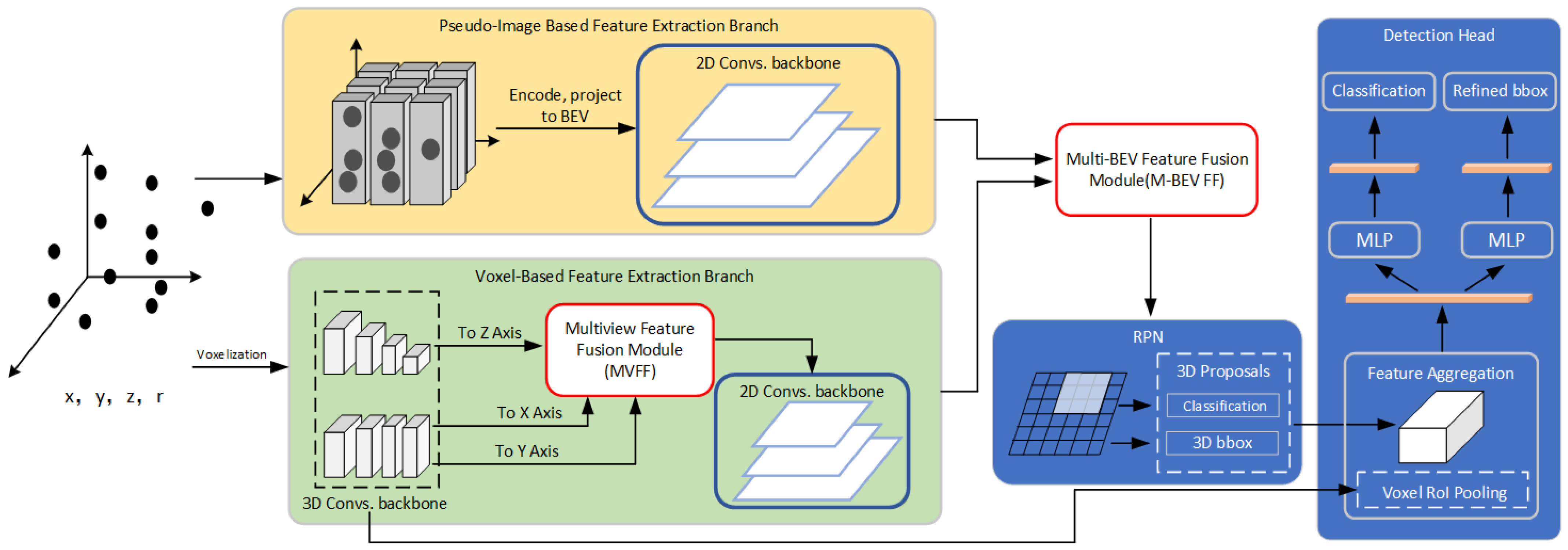
Our proposed 3D object-detection network combines the feature extraction methods of the above two networks. We use multiple methods to extract the spatial geometric features of the point clouds and then perform feature fusion. The network mainly consists of four parts: (1) the pseudo-image-based feature extraction branch; (2) the voxel-based feature extraction branch, where we propose a multiple-view feature-fusion (MVFF) module that effectively fuses the features projected on the other two views (RV and SV) into BEV features; (3) the multi-BEV feature-fusion module (M- BEV FF) which can adaptively fuse the BEV feature map generated by two branches; and (4) a detection head used to refine the detection results. The structure of our network is shown in Figure 2 and the pseudo-code of our method in PyTorch style is shown in Algorithm 1.

Algorithm 1 Pseudo-code of our proposed method in PyTorch style

Input:

1: $F_{pc}:$ Point Cloud Data 2: Initialize Hyper-parameters: 4 NVIDIA Tesla T4 GPUs, Adam optimizer, Learning Rate = 0.01, Batch Size = 2, Epochs = 80;

Output: Detected Objects(x,y,z,dx,dy,dz,heading-angle);

3: while train is True: # whether the work is training 4:     # Point Cloud Data Preprocessing 5:     $F_v$ = mean(voxelization($F_{pc}$)), $F_{pseudo-img}$ = mapToBev($F_{pc}$) 6:     # Feature Extraction and Fusion 7:     # Image Feature Extractor Module(2DExtractor) 8:     # Voxel Feature Extractor Module(3DExtractor) 9:     # Multi-view Feature Fusion Module(MVFF) 10:   # Multi-BEV Feature Fusion Module(M-BEV FF) 11:   $F_v^{{}^{\prime }}$ = 3DExtractor($F_v$) 12:   $F_{rv}$, $F_{sv}$, $F_{bev}$ = mapToXYZ($F_v^{{}^{\prime }}$) 13:   $F_{bev-voxel}$ = 2DExtractor(MVFF($F_{rv}$, $F_{sv}$, $F_{bev}$)) 14:   $F_{bev-pseudo-img}$ = 2DExtractor($F_{pseudo-img}$) 15:   $F_{bev-fusion}$ = M-BEV FF($F_{bev-voxel}$, $F_{bev-pseudo-img}$) 16:   # Detection Head 17:   prediction = refine(RPN($F_{bev-fusion}$)) 18:   loss = L(prediction) 19:   loss.backward() 20:   Update()

3.1. Assumptions of Our Method

In our method, there are several assumptions: (1) the road surface is horizontal; (2) the 3D bounding box of the detected object is parallel to the road surface; and (3) the detected object only rotates along its own Z-axis. Based on the above assumptions, the parameters that the network needs to predict are reduced from nine to seven dimensions, reducing the complexity of the network. For the detection tasks of the car, cyclist, and pedestrian categories, the above assumptions are relatively reasonable and are also common assumptions in current 3D object-detection methods [11,20].

3.2. Pseudo-Image-Based Feature Extraction Branch

This branch projects the point cloud onto the BEV to create a pseudo image and then uses the 2D feature-extraction network to extract features.

We refer to the practice of PointPillars [9] to convert point clouds into pseudo images. First, the point cloud space is discretized into cylinders. Second, according to the description in PointPillars, the original four-dimensional feature of the point cloud is expanded to a nine-dimensional feature. Third, for the points in each pillar, a small PointNet [23] network is employed for feature coding. When the coding features output by PointNet are scattered to the position of each pillar, a pseudo image with a size of $C\times H\times W$ is created, where C, H, and W represent the channel, height, and width, respectively, of the feature map.

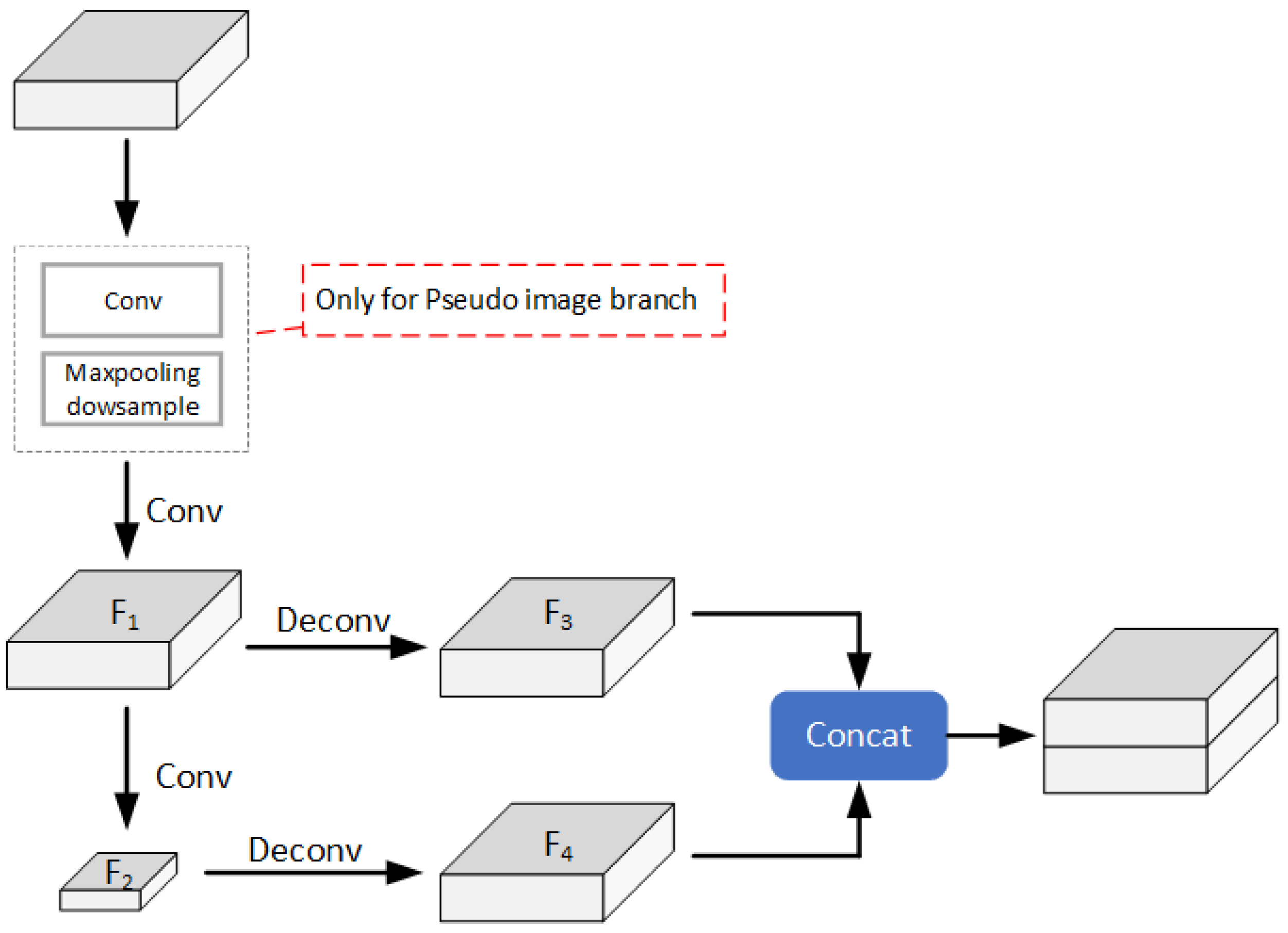
We input the created pseudo image into a 2D feature-extraction network for feature extraction. The 2D backbone network is shown in Figure 3. First, we use the convolution layer and maximum pooling layer to compress the size of the pseudo image, that is, we input the pseudo image of $C_{in}\times H\times W$ to obtain the original feature map of $C_{out}\times \frac{H}{4}\times \frac{W}{4}$. Second, the original feature map is multilayer convolved while the size of the feature map is kept unchanged to obtain the feature map $F_1$ after the first feature extraction. Third, we use multilayer convolution to further compress the size of feature map $F_1$, extract more abstract features, and obtain a new feature map $F_2$. We input feature maps $F_1$ and $F_2$ into a deconvolution layer to adjust the number of channels of $F_1$ and restore $F_2$ to the width and height dimensions of the original feature map to obtain feature maps $F_3$ and $F_4$. Last, we concatenate $F_3$ and $F_4$ in series as the output features of this branch and input them into the M-BEV FF module (Section 3.3).

3.3. Voxel-Based Feature Extraction Branch

This branch discretizes the point cloud into voxels, extracts spatial features at the voxel level, and then transforms the features into the BEV to complete the task of the feature-extraction phase. Figure 4 shows the overall structure of the voxel-based feature-extraction branch, which is divided into two parts. The first part (red part) projects voxel features in the Z direction (BEV), and the second part (blue part) projects voxel features in the X and Y directions. The multi-view feature-fusion module fuses the feature maps from three views as output.

Specifically, the point cloud is discretized into voxels according to a fixed size, with K points in each voxel. For the convenience of uniformly coding point features into voxel features, we suppose that there are N points in each voxel. If $K<N$, we fill the vacancy with 0; if $K>N$, we randomly sample N points from K points [11]. Then, the original features $(x_i,y_i,z_i,c_{raw})$ of all points in the nonempty voxel are encoded as voxel features $(f_1,f_2,\cdots ,f_N)$ by using the averaging operation. Here, $c_{raw}$ represents other attributes of the point cloud, such as reflectivity, color, and so on, in addition to the three-dimensional coordinates of the point.

To accelerate the calculation process of 3D convolution, we choose sparse convolution [12] as the main operation of feature extraction. For a feature map with input dimension $C_{in}\times D_{in}\times H_{in}\times W_{in}$, where the $D_{in}$ represents the size of the input feature map in the Z direction, we conducted four downsamplings with $1\times ,2\times ,4\times ,8\times$, and each downsampling uses 3D ResNet structure [24]. In the process of downsampling, we also introduce the residual structure and obtain a 3D feature map with shape $C_{out}\times \frac{D_{in}}{8}\times \frac{H_{in}}{8}\times \frac{W_{in}}{8}$. The 3D feature map will be projected onto the Z axis. The final output shape of the BEV feature map is $C_{bev}\times \frac{H_{in}}{8}\times \frac{W_{in}}{8}$, where $C_{bev}=C_{out}\times \frac{D_{in}}{8}$.

The above feature-extraction operation has been downsampled 4 times. With the exception of the first time, each downsampling will reduce the resolution of the feature map by half. The resolution on the Z-axis will gradually decrease; thus, some of the geometric information in this direction will be lost. We believe that the high resolution on the Z-axis can provide more geometric information in the Z-axis direction. Adding this information to the BEV feature map will help predict better 3D object proposals. Therefore, as shown in the blue part of Figure 4, we introduced another feature extraction module to enhance the Z-axis information in the BEV feature map. This part also uses sparse convolution to extract features of voxels. However, differently from the other part, the resolution is compressed only in the X and Y directions during the downsampling process, while the resolution is always fixed in the Z direction, that is, we enter a feature map with the shape of $C_{in}\times D_{in}\times H_{in}\times W_{in}$ and obtain a feature map with the shape of $C_{out}\times D_{in}\times \frac{H_{in}}{8}\times \frac{W_{in}}{8}$ after sparse convolution downsampling. Sparse convolution results are projected onto the X-axis and Y-axis to obtain the projection features in the RV and SV.

To fuse feature maps from the RV, SV, and BEV, we designed a multi-view feature-fusion module (refer to Figure 4). First, using a 1 × 1 convolution, we reduce the dimensions of the feature maps from the RV and SV to ensure consistency in their channel numbers. Second, we multiply them, model the features from three views, and obtain a feature map with the shape of $C_{bev}\times \frac{H_{in}}{8}\times \frac{W_{in}}{8}$. Third, we use the upsampling operation to adjust the number of feature map channels to an appropriate size. Last, we concatenate the above feature map with the BEV feature map obtained by sparse convolution projection of the red part, use a 2D convolution layer for fusion, and then input it into an attention module [25] to obtain the final multi-view fusion feature map.

The 2D convolution backbone also uses the structure of Figure 3 for feature extraction but removes the convolution layer and maximum pooling layer used to initially compress the size of the feature map. The final output feature map has the same width, height. and channel size as the input feature map.

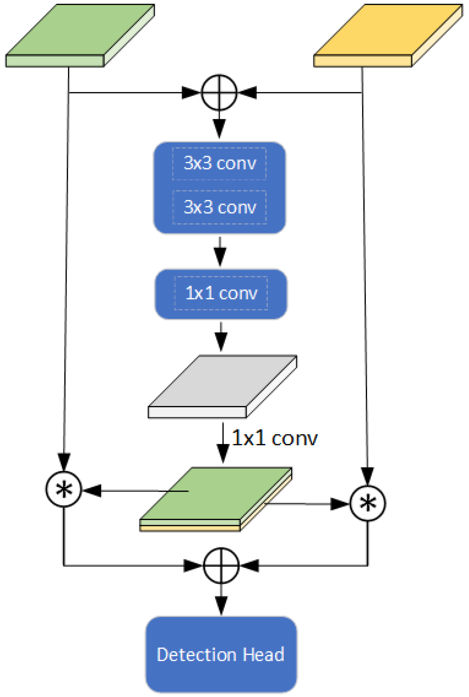
3.4. Multi-BEV Feature-Fusion Module

When multiple feature maps are fused, useful features among them can be aggregated to complement each other’s advantages [26,27]. Therefore, We developed a multi-BEV feature-fusion module (refer to Figure 5) to adaptively fuse BEV features from pseudo-image-based and voxel-based feature-extraction branches. First, we use two layers of convolution for spatial modeling and one layer $1\times 1$ for channel modeling. Second, we use a $1\times 1$ convolution layer to compress the number of channels in the feature map to two channels. We divide the feature map cuts of the two channels, use them as the BEV feature map weights from the two branches and multiply them, and then add the elements to fuse the weighted features. The multi-BEV feature fusion module effectively fuses the features extracted by different feature-extraction methods and adds richer geometric and semantic information to the BEV features to predict higher-quality 3D object proposals.

3.5. Detection Head

The detection head uses the 3D ROI output of the first stage as input and refines it to produce higher-quality detection results. Specifically, we refer to the voxel R-CNN [10] method. First, the ROI is divided into sub-voxels of the same size according to the $6\times 6\times 6$ resolution. Second, the voxel features extracted by sparse convolution are aggregated to the sub-voxels of the ROI using the voxel ROI pooling module to obtain ROI features. Last, the ROI features are flattened into feature vectors and input into two MLPs: the first MLP is utilized for confidence value prediction and the second MLP is utilized for regression refinement of the 3D bounding box parameters.

4. Experiments

In this section, we list the implementation details of the experiment and describe the dataset used in the experiment. We then show and discuss our experimental results.

4.1. Dataset

We choose the popular KITTI [28] dataset for 3D object-detection experiments. The KITTI dataset has three main object categories: cars, pedestrians, and cyclists.The data are divided into training data and test data. The training data include 7481 Lidar point cloud frames, and the test data include 7518 Lidar point cloud frames. We show the performance of the network on the val set and test set. For the val set, we divide the training data into 3712 samples for the training set and 3769 samples for the val set according to the usual practice. For the test set, we randomly select $80\%$ of the original training samples to train the network and use the remaining $20\%$ of the samples for verification as PV-RCNN [11].

4.2. Implementation Details

We set the number of training cycles to 80 and the batch size to 2 and use Adam as the optimizer. The initial learning rate is set to 0.01, and the cosine annealing strategy is applied to update it. Since the KITTI dataset only gives the object results within the camera’s field of view angle, for the three XYZ axes, we clip the point cloud space to $[0,70.4] \mathrm{m}\times [-40,-40] \mathrm{m}\times [-3,1] \mathrm{m}$. For the pseudo-image-based branch, the point cloud space is discretized into individual cylinders with a resolution of (0.1 m, 0.1 m). For voxel branches, the point cloud space is discretized into voxels using a resolution of (0.05 m, 0.05 m, 0.1 m).

4.3. Main Results

We will submit the results to KITTI’s online testing server, as shown in

Table 1. Performance comparison on the KITTI test set. The AP with 40 recall positions (R40) is selected to evaluate the 3D object detection.

Methods	Modality	FPS	Car—${AP}_{3D}(\%)$			Cyclist—${AP}_{3D}(\%)$			Pedestrian—${AP}_{3D}(\%)$
		(Hz)	Easy	Mod.	Hard	Easy	Mod.	Hard	Easy	Mod.	Hard
3D-CVF at SPA [29]	RGB + Lidar	-	89.20	80.05	73.11	-	-	-	-	-	-
CLOCs [30]	RGB + Lidar	10.0	88.94	80.67	77.15	-	-	-	-	-	-
UberATG-MMF [31]	RGB + Lidar	-	88.40	77.43	70.22	-	-	-	-	-	-
EPNet [32]	RGB + Lidar	10.0	89.81	79.28	74.59	-	-	-	-	-	-
EPNet++ [33]	RGB + Lidar	10.0	91.37	81.96	76.71	76.15	59.71	53.67	52.79	44.38	41.29
PointRCNN [14]	Lidar only	10.0	86.96	75.64	70.70	74.96	58.82	52.53	47.98	39.37	36.01
Point-GNN [15]	Lidar only	-	88.33	79.47	72.29	78.60	63.48	57.08	51.92	43.77	40.14
3DSSD [16]	Lidar only	26.3	88.36	79.57	74.55	82.48	64.10	56.90	54.64	44.27	40.23
SECOND [12]	Lidar only	30.4	85.29	76.60	71.77	71.05	55.64	49.83	43.04	35.92	33.56
PointPillars [9]	Lidar only	42.4	82.58	74.31	68.99	77.10	58.65	51.92	51.45	41.92	38.89
Part-A2-Net [34]	Lidar only	12.5	87.81	78.49	73.51	79.17	63.52	56.93	53.10	43.35	40.06
Voxel R-CNN [10]	Lidar only	25.2	90.90	81.62	77.06	-	-	-	-	-	-
Fast Point R-CNN [35]	Lidar only	-	85.29	77.40	70.24	-	-	-	-	-	-
STD [36]	Lidar only	12.5	87.95	79.71	75.09	78.69	61.59	55.30	53.29	42.47	38.35
SA-SSD [4]	Lidar only	25.0	88.75	79.79	74.16	-	-	-	-	-	-
PV-RCNN [11]	Lidar only	8.9	90.25	81.43	76.82	78.60	63.71	57.65	52.17	43.29	40.29
ours	Lidar only	14.2	87.91	80.09	76.28	80.17	65.74	58.32	45.47	39.39	36.78

and

Table 2. Performance comparison on the KITTI test set. The AP with 40 recall positions (R40) is selected to evaluate the BEV object detection.

Methods	Modality	FPS	Car—${AP}_{BEV}(\%)$			Cyclist—${AP}_{BEV}(\%)$			Pedestrian—${AP}_{BEV}(\%)$
		(Hz)	Easy	Mod.	Hard	Easy	Mod.	Hard	Easy	Mod.	Hard
3D-CVF at SPA [29]	RGB + Lidar	-	93.52	89.56	82.45	-	-	-	-	-	-
CLOCs [30]	RGB + Lidar	10.0	93.05	89.80	86.57	-	-	-	-	-	-
UberATG-MMF [31]	RGB + Lidar	-	93.67	88.21	81.99	-	-	-	-	-	-
EPNet [32]	RGB + Lidar	10.0	94.22	88.47	83.69	-	-	-	-	-	-
EPNet++ [33]	RGB + Lidar	10.0	95.41	89.00	85.73	78.57	62.94	56.62	56.24	48.47	45.73
PointRCNN [14]	Lidar only	10.0	92.13	87.39	82.72	82.56	67.24	60.28	54.77	46.13	42.84
Point-GNN [15]	Lidar only	-	93.11	89.17	83.90	81.17	67.28	59.67	55.36	47.07	44.61
3DSSD [16]	Lidar only	26.3	92.66	89.02	85.86	85.04	67.62	61.14	60.54	49.94	45.73
SECOND [12]	Lidar only	30.4	90.98	87.48	84.22	78.30	63.95	57.28	47.55	40.96	38.85
PointPillars [9]	Lidar only	42.4	90.07	86.56	82.81	79.90	62.73	55.58	57.60	48.64	45.78
Part-A2-Net [34]	Lidar only	12.5	91.70	87.79	84.61	83.43	68.73	61.85	59.04	49.81	45.92
Voxel R-CNN [10]	Lidar only	-	94.85	88.83	86.13	-	-	-	-	-	-
Fast Point R-CNN [35]	Lidar only	-	90.87	87.84	80.52	-	-	-	-	-	-
STD [36]	Lidar only	12.5	94.74	89.19	86.42	81.36	67.23	59.35	60.02	48.72	44.55
SA-SSD [4]	Lidar only	25.0	95.03	91.03	85.96	-	-	-	-	-	-
PV-RCNN [11]	Lidar only	8.9	94.98	90.65	86.14	82.49	68.89	62.41	52.17	43.29	40.29
ours	Lidar only	14.2	91.83	87.74	85.18	82.58	69.61	62.47	50.70	44.34	42.27

. Overall, our method significantly improves the detection accuracy of bicycle categories. In terms of 3D object detection, the average detection accuracy ($A{P}_{3D}$) of the easy, moderate, and hard level cyclist categories are $80.17\%$, $65.74\%$, and $58.32\%$, respectively. In terms of BEV object detection, the average detection accuracy ($A{P}_{BEV}$) of the easy, moderate, and hard level level cyclist category are $82.58\%$, $69.61\%$, and $62.47\%$, respectively.

We compared the test results with several classic 3D object-detection methods based on LiDAR point clouds. Compared with the SECOND network, our method has improved the accuracy of 3D object detection at a moderate level in three categories by $3.49\%$, $10.10\%$, and $3.47\%$, respectively, while the accuracy of BEV object detection has improved by $0.26\%$, $5.66\%$, and $3.38\%$, respectively. Compared with the PV-RCNN method, our method has improved 3D object-detection accuracy by $1.57\%$, $2.03\%$, and $0.67\%$, and BEV detection accuracy by $0.09\%$, $0.72\%$, and $0.06\%$ in the cyclist category. This discovery indicates that our algorithm supplements some of the feature information required to detect cyclist category objects on the basis of the original method. It can be noted that our method performs poorly in the detection tasks of the car and the pedestrian. We will discuss this problem later.

Table 1 also shows a comparison of the average detection runtime between different algorithms. Because our network has introduced more modules and parameters, the number of detection frames has decreased to 14.2Hz, but it can basically meet actual usage requirements.

We set 40 recall locations and IoU threshold values of 0.7 (for car) and 0.5 (for cyclist) and calculated the AP of 3D object detection of the network on the val set of the KITTI dataset for further comparison.

Table 3. Performance comparison on the KITTI val set with AP calculated by 40 recall positions for car class.

Methods	Car—${AP}_{3D}(\%)$			Cyclist—${AP}_{3D}(\%)$			Pedestrian—${AP}_{3D}(\%)$
	Easy	Mod.	Hard	Easy	Mod.	Hard	Easy	Mod.	Hard
SECOND [12]	90.55	81.61	78.61	82.96	66.74	62.78	55.94	51.14	46.17
PV-RCNN [11]	91.89	84.52	82.43	91.57	72.64	69.23	68.35	60.52	55.11
Voxel R-CNN [10]	93.09	85.04	82.31	92.10	73.28	70.13	63.27	56.94	51.56
ours	91.65	84.31	82.20	93.58	74.57	71.10	65.86	59.39	54.61

shows the specific calculation results: our method has a detection accuracy of $84.31\%$, $74.57\%$, and $59.39\%$ at the moderate level for three categories, performing well on detection tasks in the cyclist and pedestrian, but not well on detection in the car. According to the results in Table 3, our method is comprehensively superior to SECOND, and the accuracy of moderate level detection for the three categories improve by $2.70\%$, $7.83\%$ and $8.25\%$. At the three levels of the cyclist category, our method is $2.01\%$, $1.93\%$, and $1.87\%$ higher than PV-RCNN’s AP, $1.48\%$, $1.29\%$, and $0.97\%$ higher than the original Voxel R-CNN, with an obvious improvement effect. At three levels of pedestrian category, our method is $2.49\%$, $1.13\%$ and $0.50\%$ lower than the original PV-RCNN, but $2.59\%$, $2.42\%$ and $3.05\%$ higher than Voxel R-CNN using the same second stage network. At the three levels of the car category, the performance of our method is similar to PV-RCNN, but lower than Voxel R-CNN with $1.44\%$, $0.73\%$, and $0.11\%$.

Although our method has effectively improved the detection results of the cyclist category, combined with the comparison results in Table 1, Table 2 and Table 3, our method has not performed well in the detection task in the automobile category. There are several possible reasons for this. First, we project the voxel features to the X and Y directions, and then integrate the projection feature maps of the X and Y directions into the BEV feature map to supplement the geometric feature information missing from the BEV feature map due to dimension compression. Because the volume of cyclists and pedestrians in the three-dimensional space is small, and the projection area under the BEV perspective is also small, the detection network that only relies on the BEV perspective learns less features related to these two objects. In addition, in the KITTI dataset, the number of labels in the car category is three to four times that of cyclist and pedestrian. This imbalance makes it more difficult for the network to learn feature information related to cyclist and pedestrian detection tasks, making features related to car category dominant. Although our network has learned more features that are helpful for cyclist and pedestrian detection tasks, these features have certain side effects on car category detection tasks. Therefore, the detection performance of the cyclist and pedestrian has improved, while the detection performance of the car has slightly decreased.

In addition, in Table 1 and Table 2, the performance of our network in the pedestrian category is not very good. We believe there are two main reasons for this. First, the 3D spatial features extracted from our network are only voxel features. Due to the small volume of pedestrians in 3D space, it is difficult to extract effective features only with voxels, so the networks that perform well in pedestrian categories in Table 1 and Table 2 are extracted original point features, or both voxels and original point features are extracted and fused. Second, the second stage network we selected is not suitable for the detection of pedestrians.The results in Table 3 show that at three levels of pedestrian category, the original Voxel R-CNN’s $A{P}_{3D}$ is $63.27\%$, $56.94\%$, and $51.56\%$, respectively. And our method is $2.59\%$, $2.42\%$, and $3.05\%$ higher than the original Voxel R-CNN’s $A{P}_{3D}$.This means that our method has indeed learned more features of the pedestrian category, which proves our view.

4.4. Ablation Study

Table 4. Effect of the two modules that we propose on the performance of the KITTI val set. PI-based is pseudo-image based feature extraction. V-based is Voxel-based feature extraction. “MV” and “M-BEV” represent the multi-view feature fusion module and multi-BEV feature fusion module, respectively. The results are evaluated with the average precision calculated by 40 recall positions for the cyclist class.

Methods	PI-Based	V-Based	MV	M-BEV	Car—${AP}_{3D}(\%)$			Cyclist—${AP}_{3D}(\%)$			Pedestrian—${AP}_{3D}(\%)$
					Easy	Mod.	Hard	Easy	Mod.	Hard	Easy	Mod.	Hard
(a)	✓				87.89	78.28	75.46	83.07	64.42	60.09	53.29	47.77	43.88
(b)		✓			93.09	85.04	82.31	92.10	73.28	70.13	63.27	56.94	51.56
(c)	✓	✓		✓	91.57	82.64	81.86	92.47	73.29	68.71	65.50	58.97	54.59
(d)	✓	✓	✓	✓	91.65	84.31	82.20	93.58	74.57	71.10	65.86	59.39	54.61

shows the actual impact of the two modules that we proposed on the detection results. The AP is evaluated at three levels in the cyclist category.

Methods (a) and (b) are the baselines for the outcome evaluation. In method (a), only the feature extraction branch based on the pseudo image is retained, and the whole network degenerates into a single-stage object-detection network. Method (b) only retains the voxel-based feature-extraction branch.

In method (c), we introduce our multi-BEV feature fusion module to adaptively fuse BEV feature maps from two branches. Compared with method (b), method (c) has significantly improved performance in pedestrian detection tasks, with $A{P}_{3D}$ improving $2.23\%$, $2.03\%$ and $3.03\%$ respectively, verifying the practical role of our multi-BEV feature fusion module. However, method (c) performs poorly in the detection tasks of the car and the cyclist.

Method (d) is based on method (c), and we have added the multi-view feature fusion module. Compared to method (c), on all detection tasks, $A{P}_{3D}$ have a certain improvement effect. Especially for the cyclist detection task, $A{P}_{3D}$ has improved $1.11\%$, $1.28\%$ and $2.39\%$, respectively. The results show that our multi-view feature fusion module can effectively fuse RV and SV features with BEV features, supplement some missing feature information in BEV feature maps, and obtain better 3D target-detection results. However, for the overall network, as we discussed in Section 4.3, although our method has learned more features related to pedestrian and cyclist, it has somewhat reduced the detection performance of car categories.

5. Conclusions

In this work, we propose a multi-view joint learning and BEV feature-fusion network that combines BEV features extracted from different point cloud representations. The backbone of the feature extraction network consists of two branches. The pseudo-image-based feature-extraction branch encodes the point cloud and projects it onto the BEV perspective to directly extract BEV features. The voxel-based feature-extraction branch discretizes the point cloud into voxels. After spatial sparse convolution, the feature is projected onto the RV, SV, and the BEV. The features of the three perspectives are fused in the MVFF module to obtain BEV features. Then, the network adaptively fuses the BEV features of the two branch outputs through the M-BEV FF module to generate a 3D ROI, which is refined in the second stage of the network. According to the experimental results of the test set and the val set of the KITTI dataset, our network has successfully improved the detection results for the cyclist and pedestrian categories, which shows the effectiveness of our proposed network structure and the new modules.

Although our network performs well in bicycle and pedestrian detection tasks, there are also certain limitations. For example, the network improves the detection performance of bicycle and pedestrian categories while reducing the detection performance of vehicle categories. Therefore, it is worth considering using a better fusion strategy to fuse features from multiple views, including RV, SV, BEV, and perform joint learning to obtain fusion features that contain more information, achieving better 3D object-detection results.In addition, because our network has two feature-extraction branches, it consumes a large amount of computing resources and time resources in feature extraction. Therefore, we can also consider improving the network in the future to ensure that the detection accuracy is equivalent to or slightly lower than the existing detection accuracy, while reducing complexity or computing costs, so that the network has better practical performance.