A Comprehensive Review of GNSS/INS Integration Techniques for Land and Air Vehicle Applications

Abstract

Navigation systems are of interest for applications in both civilian and military vehicles. Satellite navigation systems and inertial navigation systems are the most applied in this area. They have complementary properties, which has led to a trend of integrating these systems. At present, there are several approaches to GNSS/INS integration: loosely coupled, tightly coupled and deeply coupled and many approaches to their modifications in dependence of application and arising problems with measurements, such as lack of GNSS measurements or poor quality of GNSS and INS measurements. This article presents an extensive review of the available modern approaches and their modifications for integrating INS and GNSS measurements, arranging them and highlights the main problems arising for the considered type of integration approach. The article includes a review of various integration tools based on the Kalman filter and intelligent systems, INS mechanization and features of development of an INS measurement error model that is necessary for integration, the main problems of GNSS/INS integration and a comparative description of the solutions proposed by the authors for solving these problems. The findings of this work are useful for further research in the field of inertial and satellite navigation, as well as for engineers involved in the practical implementation of integrated GNSS/INS systems.

1. Introduction

The field of application of autonomously functioning navigation systems is growing every day and includes applications in both civilian and military vehicles. Generally, navigation systems can be divided into inertial navigation systems and satellite navigation systems [1,2]. Inertial navigation systems determine the current position of an object based on the measurement of the velocity and acceleration of the object. Satellite navigation systems determine the position of an object based on measurements related to other objects, in particular the moments of receiving a synchronized signal from navigation satellites that is used for calculation of the ranges and pseudoranges of navigation satellites [1].

Satellite navigation systems (SNS) based on GNSS receiver subject to the availability of measurements from four navigation satellites can provide an accuracy in determining the position of an object up to 20 m, and accuracy improvement is possible through the use of differential correction methods [3]. However, in cases when the satellite navigation system consists of one navigation GNSS receiver with one antenna, it is impossible to estimate the angular position of the object, which is a disadvantage in cases of application to flying objects. In addition, satellite navigation systems are quite sensitive to external conditions: the presence of obstacles in the form of vegetation and civil buildings, as well as blocking the signals of navigation satellites [3,4].

Inertial navigation systems (INS) are devices that are completely autonomous from external conditions. They include sensors for measuring velocity and acceleration [5,6]. Modern inertial navigation systems are platform INS mechanically stabilized using a special platform and strapdown INS (SINS) that are numerically stabilized using special algorithms implemented in an additional computing device of the navigation system [6]. The raw output of the SINS is represented by the angular velocity and the specific force in the associated coordinate system. The position and attitude of the object are determined by integration using initial conditions. Thus, inertial navigation systems make it possible to calculate the position of an object and its attitude. However, inertial navigation systems with all their advantages have a significant drawback, which is that their accuracy decreases over time. The presence of an error in the INS measurements leads to a large error in determination of the object position when integrating the measurement data [6,7].

Thus, satellite and inertial navigation systems have complementary properties, which has led to a trend of integrating these systems to obtain reliable autonomous navigation systems. Currently, there are many techniques of SNS/INS integration. The simplest and most obvious approach is to use the output data of the SNS on the position and velocity of the object as initial conditions for the INS [7,8]. This technique is called INS with GPS resetting. However, this technique has several disadvantages. In the most general case, a GNSS with a single antenna provides only an estimation of the position and velocity of an object, which will be used as initial conditions in the INS, while the initial conditions for the angular velocity and attitude will be selected. An inaccurate choice of initial conditions for the attitude for the INS will lead to an unlimited accumulation of errors. In addition, the “correction” of the initial conditions for the INS is possible at those moments when the SNS measurements are available. As is known, the operation of the SNS can be disrupted due to intentional signal suppression or unintentional suppression associated with the presence of obstacles. In this regard, using more advanced integration techniques is preferable.

Traditionally, more advanced integration techniques are based on the use of the Kalman filter as a tool for estimating INS error based on the use of SNS measurements [8]. This approach is called complementary or GPS-aided INS.

The first technique based on the GPS-aided INS approach is called loosely coupled integration technique. In a loosely coupled integration system, when obtaining measurements of the SNS in the form of the velocity and position of the object, they are used to construct a complementary vector of measurements of the Kalman filter, which estimates the error of the INS. In the absence of SNS measurements, the estimated error of the INS is equal to the predicted error of the INS in the Kalman filter. The resulting INS error estimate is then subtracted from the INS measurements, thereby providing the output parameter of the integrated system. In this case, the complementary measurement vector is the difference between the measurements of the position of the object determined by the SNS and the INS [7,8,9,10,11,12]. That is, the SNS has already implemented a solution to the navigation problem of determining the position and velocity of an object in the presence of measurements from four satellites. This integration scheme is the simplest but has obvious drawbacks. Namely, if signals from four navigation satellites are unavailable, the SNS will not determine the position of the object and then the integrated system works as INS, which, as is known, accumulates an error over time [7]. Despite this, the loosely coupled scheme is the most commonly implemented integration scheme, since, in fact, separate data of INS and SNS are used to “correct” the error of the integrated SNS/INS system. This allows the use of any commercially available SNS and INS. Currently, some modifications of the loosely coupled integration system are known. For example, in [13], it is proposed to introduce a model of fictitious navigation satellites having a certain position in space. It is proposed to use satellites that are not currently in sight, as well as artificial (fictitious) navigation satellites. In [14], a quasi tightly coupled integration technique based on a loosely coupled scheme is proposed. In this case, the Kalman filter is also used to estimate the INS error. Two processes are added to the integration scheme: calculation of the a priori position of the GNSS receiver installed on the object based on the current position and the attitude determined by the INS. Further, the SNS makes a correction of the obtained a priori position. In [15], it is proposed to use a multilayer perceptron neural network in combination with the Kalman filter for predicting and estimating the position of GNSS satellites when they are not available.

The second technique based on the GPS-aided INS approach is called the tightly coupled integration technique. A tightly coupled integration system also uses a Kalman filter to estimate the error of the INS. However, in contrast to the loosely coupled integration system, the GNSS measurements are used here to estimate the pseudorange, carrier phase or Doppler shift which are then used to construct a complementary measurement vector in the Kalman filter [11,16,17,18]. Accordingly, the complementary measurement vector is the difference between the pseudoranges, carrier phase or Doppler shift measurements determined by the INS and GNSS [7,8]. This integration scheme is more difficult to numerically implement than a loosely coupled scheme since it is necessary to implement the calculation of ephemeris, the GNSS receiver clock model, etc., to determine the pseudorange, carrier phase or Doppler shift. However, it allows to carry out a partial “correction” of the INS error in the presence of limited GNSS measurements since the measurements in the Kalman filter are updated even when measurements from one navigation satellite are available [7,11].

The third basic technique is called the deeply (or ultra-tight) coupled integration technique that is implemented at the hardware level. A deeply coupled system is an extended version of a tightly connected integration system by supplementing the process of SNS operation with INS functionality [7]. In particular, the integration of INS and SNS measurements is performed at the level of combining GNSS RF samples with inertial measurement samples [7,19].

In general, even in case of using the tightly coupled and deeply coupled integration schemes, it cannot help reducing the accuracy of the integrated system when GNSS signals are unavailable. To solve this problem, many developers offer several approaches. One of the approaches is the use of the ZUPT (Zero Velocity Update) method, based on curve approximation methods for estimating the error in determining the velocity and position of an object using INS [20]. When implementing the proposed approach for moving objects, it may be difficult to approximate curves due to the presence of many rapidly changing parameters, such as time, acceleration and motion trajectory. In most cases, this approach is applicable to objects that make many stops so that the algorithm can work in static mode. For the most part, it is more applicable to the implementation of an integrated INS/GNSS system for pedestrians. Approaches based on the use of additional equipment, such as computer vision [21], odometer [22] or odometer and compass [23], are also much applicable. In particular, in [22], a street return algorithm was proposed that makes it possible to refine the position determined using the INS in the absence of GNSS measurements. In [23], an upgrade and improvement of this algorithm using a compass is proposed. Moreover, methods based on neural networks [24,25] are widely used. In [24], it is proposed to use a neural network to predict INS errors in determining the velocity and position of an object during restrictions on access to GNSS signals. The authors of [24] propose to use a neural network for simulation of temporarily absent GNSS signals. In connection with the effect of multipath of GNSS signal, as well as with the effects of the ionosphere and troposphere [5,26], there is a problem associated with the need to reduce the outliers, for example, for pseudorange, leading to a deterioration in the positioning accuracy of an object [27]. To reduce the outliers, the authors of [27] propose a method for estimating the measurement error, which involves the use of a nonlinear filter in real time. In [28], an adaptive robust Kalman filter is proposed that makes it possible to eliminate low-quality measurements and outliers and improve the accuracy of determining the position and velocity of an object.

Approaches based on accurate modelling and estimation of INS stochastic errors are also used to improve the accuracy of integrated INS/GNSS systems. Several methods are proposed in open publications, in particular methods based on the use of an autoregressive model, a Gauss–Markov model [29], Allan variance [30] and a combination of the proposed approaches [31]. The paper [32] proposes an INS error model based on two tools: a technique for modeling nonlinear errors called fast orthogonal search (FOS) and the support vector machine (SVM) to estimate and eliminate the errors of the INS gyro sensor without the need to use the output parameters of the Kalman filter to estimate the error of the INS when GNSS measurements are unavailable. Other tools, such as the robust Kalman filter [33], unscented Kalman filter [34,35] and complex algorithms based on neural networks [36,37,38], are also used for improving the accuracy of the integrated SNS/INS system.

The development of integrated INS/GNSS systems in relation to land vehicle is based on the principles listed above. The Kalman filter [6,39,40], deeply coupled [40], loosely coupled [41], and tightly coupled [42] integration schemes are used as the main tool for integration. The main features of the application of integrated INS/GNSS systems to vehicles are the limitations caused by the trajectory of motion within the urban space. In particular, it is assumed that, when a ground vehicle moves, it does not slip off the trajectory and does not bounce, that is, the motion occurs in a constant direction; the velocity of the object in the direction perpendicular to the direction of its motion is equal to zero. Taking into account the considered kinematic limitations and features of the vehicle dynamics will improve its positioning accuracy. If we do not consider the proposed restrictions on maintaining the direction of motion, a lever arm effect arises due to the fact that the INS and GNSS are installed in different places on the vehicle, which leads to a difference in the velocity measurements of the INS and GNSS [6]. These limitations can be considered in the Kalman filter to obtain better positioning accuracy. As shown in [43], the constrained Kalman filter provides better accuracy than the traditional filter. In [44], the error from the lever arm effect is included in the INS error vector for estimation in the Kalman filter. Further, in [45,46], the authors continued their work and assessed the influence of the lever arm for the integrated SNS/INS system installed on a car driving along a given trajectory. The research results showed that the estimation of the effect of the lever arm and the angular position of the object are quite sensitive to the trajectory of the object and the nature of its motion. In [47], a new way of specifying the lever arm in the form of spherical coordinates in the Kalman filter was proposed to estimate its influence. In [48], it is proposed to use “virtual” measurements of the lever arm for use in the Kalman filter, which estimates the error of the INS.

The development of integrated INS/GNSS systems for air transport, in particular unmanned aerial vehicles, also uses the main integration tools, such as the Kalman filter. The main difference from ground transport is that the UAV has more complex dynamics and, accordingly, a trajectory. In the works of the authors, both loosely coupled and tightly coupled integration schemes are used. In particular, in [49], the implementation of a loosely coupled navigation system for an agricultural UAV is considered. In [50], both a loosely coupled and a tightly coupled system for a helicopter-type UAV under various conditions imposed on the flight path, as well as under various conditions of availability of GNSS signals, is considered. The problem of development of an integrated system for helicopter-type UAVs in the presence of a magnetic sensor in addition to the integrated INS/SNS system is considered in [51]. In [52], the problem of creating a tightly coupled system for an UAV copter based on commercially available INS and GNSS navigation sensors with multiple antennas is considered. The main advantage of this work consists of using double differences instead of single difference. It helps to remove the clock errors. Although [52] is out of the scope of this article, devoted to the use of single-antenna GNSS receivers, it deserves attention as one of the interesting engineering approaches to the design of integrated systems. In [53], a tightly coupled system based on a broadband GNSS receiver and an INS is considered using the factor graph optimization method as an integration tool, allowing you to reduce the problem of finding a navigation solution to a non-linear least squares method, which improves the accuracy of the UAV navigation system in indoor conditions, with a high probability of the influence of the multipath effect in the absence of direct radio visibility. The papers [54,55] consider budget integrated SNS/INS systems for UAVs based on cheap commercially available INS with a low accuracy included strapdown system. Works [56,57] are devoted to improving the integrated INS/SNS system by developing an adaptive Kalman filter that is improved using machine learning to classify GNSS errors. For air transport applications, where safety is a concern, it is important to improve the reliability of measurements conditioned by the integrity of the measurements. Integrity of GNSS measurements can be broken by various factors, including environmental factors, atmospheric effects and interference. To provide reliability and integrity of measurements, one can use augmentation systems, receiver autonomous integrity monitoring (RAIM), redundancy, etc. [58,59].

Thus, the main problems faced by developers of integrated systems are as follows:

−

unavailability of GNSS signals, leading to the accumulation of errors in determining the position and velocity of the object due to the functioning of the integrated system in the INS mode;

−

the presence of outliers and violation of integrity of GNSS measurements (for example, pseudorange) due to multipath effect, ionospheric and tropospheric effects, interference, environmental factors, which can lead to instability of SNS measurements;

−

the presence of errors and effects in INS measurements due to the characteristics of the sensors, such as static and dynamic errors (bias) of the INS, the lever arm effect, crosslinks, etc.

This paper considers the analysis of the current state in the field of available approaches for INS/GNSS integration for accurate determination of the position and velocity of moving objects. The focus will be on integrated systems designed for mobile land and aerial vehicles, on the main factors affecting the accuracy and functionality of the integrated system and on the issues for solving of related problems. The Section 2 discusses various approaches to INS/GNSS integration based on filters and measurements. The Section 3 discusses the functionality of GNSS and INS to determine the position and velocity of an object and the features of development of an INS measurement error model that are necessary for integration. The Section 4 considers the main problems of GNSS/INS integration, a comparative description of the solutions for these problems proposed by the authors and their analysis. The Section 5 contains conclusions and recommendations.

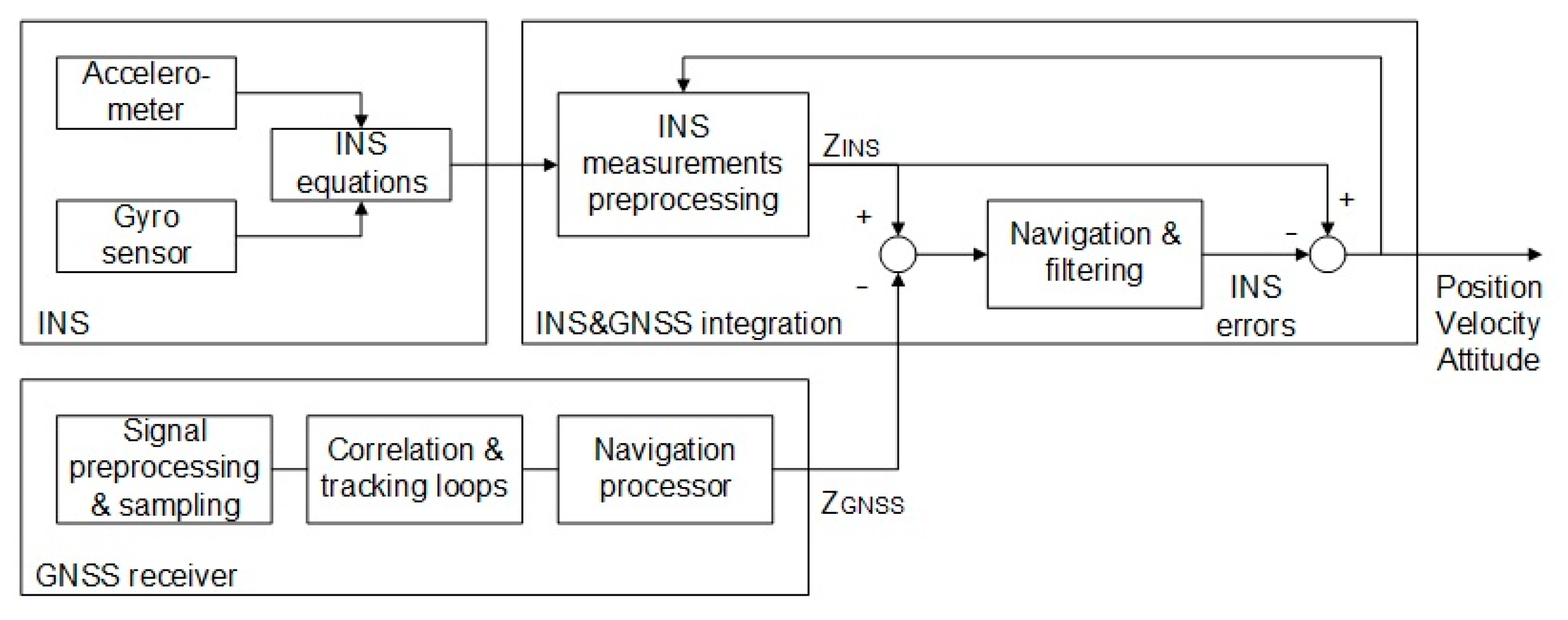
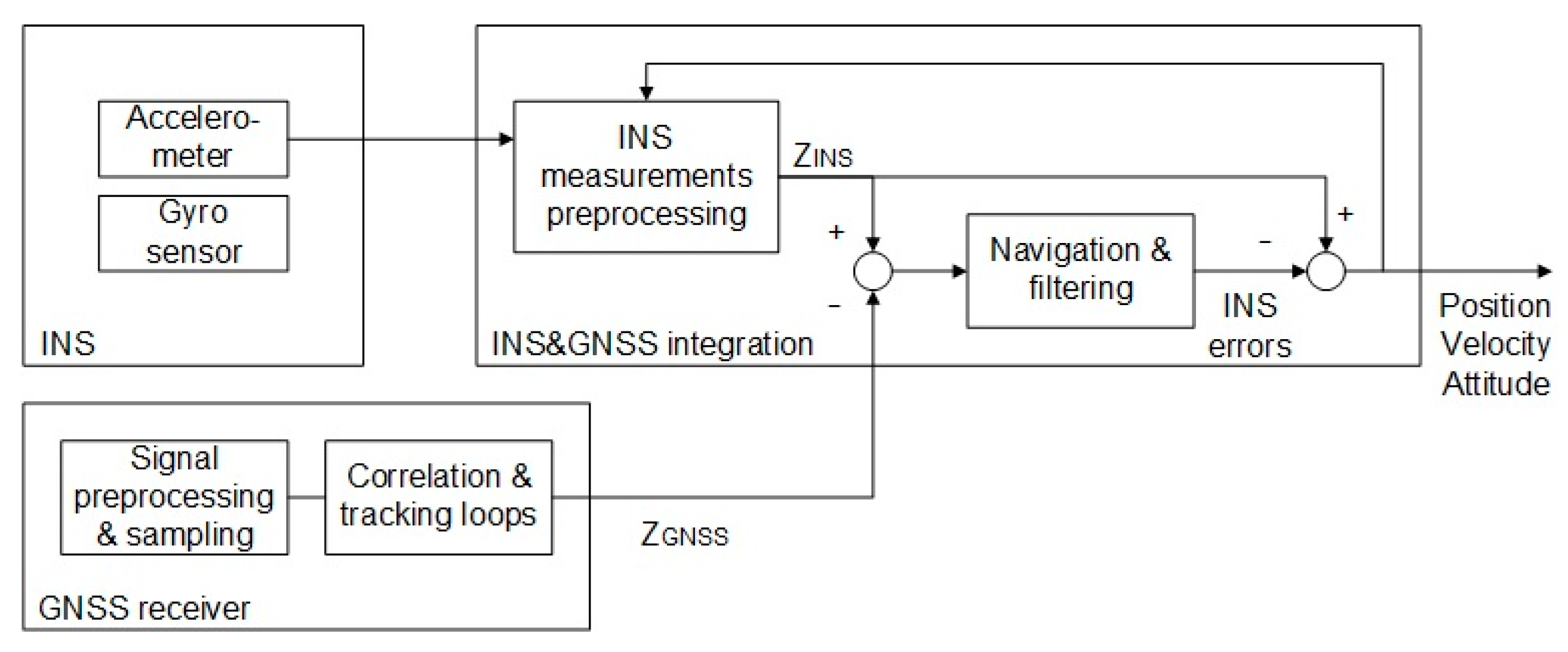
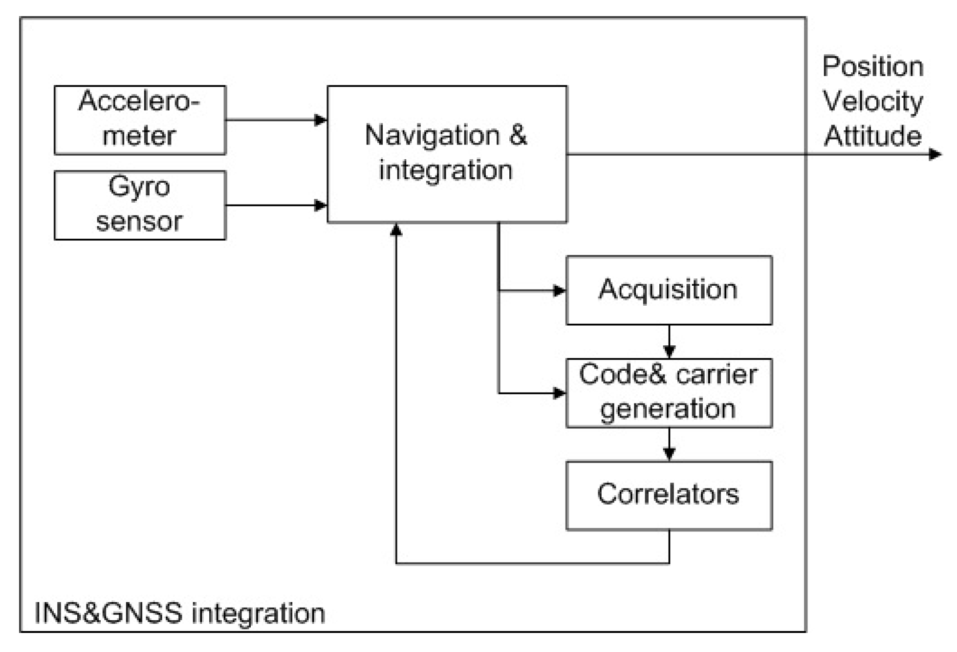
2. GNSS/INS Integration Techniques

In most cases, INS/SNS measurements are integrated using the filtering algorithm in loosely coupled, tightly coupled and deeply coupled integration schemes. In loosely coupled and tightly coupled integration schemes, the difference between INS and SNS measurements is used to estimate the INS error, and then the INS navigation solution is corrected with resulting INS error estimate [7,8] (Figure 1 and Figure 2). In the case of a loosely coupled scheme, the difference between the position and velocity measurements obtained by GNSS and INS is used. In the case of a tightly coupled scheme, the difference between the pseudorange, carrier phase or Doppler shift measurements obtained by GNSS and INS is used.

In the deep integration scheme, GNSS receiver and INS are not independent devices. GNSS measurements are used to estimate INS errors and INS measurements are used to aid GNSS receiver tracking loops (Figure 3). In [19], the deep integration approach is considered that starts fusion of GPS and inertial data at the earliest processing stage possible by combining radiofrequency GNSS samples with sampled INS measurements. Obtained integrated signals are applied to estimate GNSS solution, including code phase, carrier Doppler frequency shift and carrier phase. After that, these GNSS estimates are used in Kalman filter to update INS error state.

As can be noted, deep integration is performed at the level that requires the access to the GNSS receiver source code, which is usually available only for receiver manufacturers. For this reason, we have not considered this type of integration in this manuscript and have studied in detail the loosely coupled and tightly coupled integration schemes that are more available to implementation by most GNSS users.

From the review, the Kalman filter is the most used integration tool. The Kalman filter is implemented according to the standard scheme. At the first stage, the estimate of the INS error vector and the covariance matrix for the INS error are predicted based on the available measurements of the INS and SNS. At the next stage, after receiving the measurements, the predicted INS measurement error vector and the covariance matrix are corrected.

Since the INS and SNS operate at different frequencies, the integration in the Kalman filter is performed at the moments ${t_k=t}_{GNSS}$ when the GNSS measurements are obtained. The Kalman filter algorithm is as follows:

(1)

Predicting the estimate of the INS measurement error vector.

Since, after receiving each new SNS measurement, the INS measurements are corrected, the best current estimate of the INS error is zero $\delta {\widehat{\mathit{x}}}_{k/k}=0$. Then, the predicted score at $t_{k+1}$ is:

$$\delta {\widehat{\mathit{x}}}_{k+1/k}=0$$

(1)

The predicted value of the covariance matrix at $t_{k+1}$ is determined based on the expression:

$${\mathit{P}}_{k+1/k}={\mathit{\Phi }}_k{\mathit{P}}_{k/k}{\mathit{\Phi }}_k+{\mathit{Q}}_k$$

(2)

where ${\mathit{P}}_{k/k}$ is the covariance matrix at the moment of time $t_k$, ${\mathit{\Phi }}_k=\mathit{I}+\mathit{F}\Delta t$, ${\mathit{Q}}_k=\mathit{G}\mathit{Q}{\mathit{G}}^T\Delta t$, $\Delta t=t_{k+1}-t_k$, matrices $\mathit{F}$ and $\mathit{Q}$, respectively, depend on the INS measurement error model and the type of the INS measurement error vector.

(2)

Correction of the predicted INS measurement error vector.

To perform this step, it is necessary to update the measurements of the INS and SNS and calculate their difference $\delta {\widehat{\mathit{z}}}_{k+1}$. After that, update the matrix ${\mathit{H}}_{k+1}$ and calculate the coefficient matrix:

$${\mathit{K}}_{k+1/k+1}=\left({\mathit{P}}_{k+1/k}{\mathit{H}}_{k+1}^T\right){({\mathit{R}}_k+{\mathit{H}}_{k+1}{\mathit{P}}_{k+1/k}{\mathit{H}}_{k+1}^T)}^{-1}$$

(3)

where the matrix ${\mathit{H}}_{k+1}$ depends on the type of SNS and INS measurements, ${\mathit{R}}_k$ is the covariance matrix built on the basis of knowledge of the measurement error of the SNS.

After that, it is possible to correct the estimation of the INS measurement error vector and the covariance matrix:

$$\delta {\widehat{\mathit{x}}}_{k+1/k+1}={\mathit{K}}_{k+1/k+1}\delta {\widehat{\mathit{z}}}_{k+1}$$

(4)

$${\mathit{P}}_{k+1/k+1}=[\mathit{I}-{\mathit{K}}_{k+1/k+1}{\mathit{H}}_{k+1}]{\mathit{P}}_{k+1/k}.$$

(5)

The considered algorithm is common for most integration schemes. The vector of the difference between the measurements of INS and SNS will differ. In particular, for a loosely coupled integration scheme, the vector is formed based on the difference between the position and velocity measurements obtained by GNSS and INS [8]:

$$\delta {\widehat{\mathit{z}}}_{k+1}=\delta {\widehat{\mathit{z}}}_{k+1}^{GNSS}-\delta {\widehat{\mathit{z}}}_{k+1}^{INS}=\left[\begin{array}{ccc}1& 0& 0\\ 0& 1& 0\\ 0& 0& 1\end{array}\right]\left[\begin{array}{c}\delta n\\ \delta e\\ \delta d\end{array}\right]+\mathbf{\eta }$$

(6)

where $\delta \mathit{p}=\left[\delta n,\delta e,\delta d\right]$ is the error vector of the object position in the local coordinate system NED (North, East, Down) or ENU (East, Nort, Up), $\mathbf{\eta }$ is the noise.

In the case of a tightly coupled integration scheme, this vector has the form [8]:

$$\delta {\widehat{\mathit{z}}}_{k+1}=\left[\begin{array}{c}{h}_1{C}_n^e, 1\\ h_2{C}_n^e, 1\\ \begin{array}{c}\dots \\ \begin{array}{c}{h}_m{C}_n^e\\ 1\end{array}\end{array}\end{array}\right]\left[\begin{array}{c}\delta n\\ \delta e\\ \begin{array}{c}\delta d\\ b_u\end{array}\end{array}\right]$$

(7)

where ${\mathit{h}}_i$ is the vector in the direction from the satellite to the object (line of sight vector); $b_u$ is the clock bias in GNSS measurements.

Accordingly, depending on the type of vector, $\delta {\widehat{\mathit{z}}}_{k+1}$ the matrix ${\mathit{H}}_{k+1}$ will differ.

The measurement error vector $\delta \mathit{x}$ usually includes the error in determining the position of the object $\delta \mathit{p}=\left[\delta n,\delta e,\delta d\right]$ in the local coordinate system NED/ENU, the error in determining the velocity of the object $\delta \mathit{v}=\left[\delta v_n,\delta v_e,\delta v_d\right]$ in the local coordinate system ENU, the error in determining the angular position of the object $\delta \mathit{e}=[\delta \varphi ,\delta \theta ,\delta \psi ]$, the static bias of the accelerometer ${\mathit{b}}_a$ and the static bias of the gyro sensor ${\mathit{b}}_g$. Accordingly, for a given measurement error vector $\delta \mathit{x}=\left[\delta \mathit{p},\delta \mathit{v},\delta \mathit{e},{\mathit{b}}_a,{\mathit{b}}_g\right]$, there is its own measurement error model described by differential equations and the corresponding matrix $F$, for example, given in equation 3.68 in [8], in equation 6.97 [10], in equation 12.28 in [60]. A similar model was used in most of the available papers [2,4,5,6,11]. In [48], the error due to the lever arm effect is included in the measurement error model for its subsequent evaluation in the Kalman filter. Some authors include additional parameters for evaluation in the Kalman filter; for example, in [61,62], in addition to static bias for the accelerometer and gyro sensor, dynamic biases $\sigma {\mathit{b}}_a, \sigma {\mathit{b}}_g$ are also introduced into the measurement error model, respectively; the state vector of the Kalman filter takes the form $\delta \mathit{x}=\left[\delta \mathit{p},\delta \mathit{v},\delta \mathit{e},{\mathit{b}}_a,{\mathit{b}}_g,\sigma {\mathit{b}}_a,\sigma {\mathit{b}}_g\right]$. It contributes to obtaining the most complete model but greatly complicates the algorithm.

To improve the reliability and performance of the integrated INS/SNS system, various modifications of the integration algorithm based on the Kalman filter are used. For example, the use of neural networks for learning to predict the motion of GNSS satellites during the periods when their measurements are unavailable [15,24], the use of a robust Kalman filter to eliminate outliers in the measurements of the position and velocity of GNSS satellites, unscented Kalman filter [35,63,64]. The accuracy of various implementations of loosely coupled and tightly coupled integrated systems in terms of mean error or root mean square error (RMSE) characterizing the deviation of estimated data from reference data are provided in

Table 1. Comparative characteristics of loosely coupled integrated GNSS/INS systems in terms of mean error or RMSE and methods used to improve the operation of integrated INS/SNS systems.

Publication	RMSE/Mean Position [NED]/ [Lat,Lon,Alt]	RMSE/ Mean Position 3D	RMSE/Mean Velocity $[{\mathit{v}}_{\mathit{N}}$$, {\mathit{v}}_{\mathit{E}}$$, {\mathit{v}}_{\mathit{D}}]$	RMSE/ Mean Velocity 3D	RMSE/ Mean Attitude [P,R,Y]	Integration Technique	Improving Method
Integrated INS/GPS Navigation System [2]	RMSE N = 2.379 m E = 1.901 m D = 3.438 m	-	RMSE $v_N=0.3067 \mathrm{m}/\mathrm{s}$ $v_E=$ 0.1048 $\mathrm{m}/\mathrm{s}$ $v_D=0.9269$ m/s	-	-	15-state KF	Update rate increasing
The Performance Analysis of a Real-Time Integrated INS/GPS Vehicle Navigation System with Abnormal GPS Measurement Elimination [5]	RMSE N = 5.9 m E = 6.0 m D = 22.3 m	RMSE 23.8 m	RMSE $v_N=0.35 \mathrm{m}/\mathrm{s}$ $v_E=$ 0.54 $\mathrm{m}/\mathrm{s}$ $v_D=0.22$ m/s	RMSE 0.68 m/s	RMSE $P={0.26}^{°}$ $R={0.15}^{°}$ $Y={9.02}^{°}$	15-state KF	-
Performance analysis of GNSS/INS loosely coupled integration systems under GNSS signal blocking environment [11]	RMSE N = 0.01 m E = 0.02 m D = 0.011 m	-	RMSE $v_N=0.005 \mathrm{m}/\mathrm{s}$ $v_E=$ 0.005 $\mathrm{m}/\mathrm{s}$ $v_D=0.006$ m/s	-	RMSE $P={0.0096}^{°}$ $R={0.007}^{°}$ $Y={0.007}^{°}$	15-state KF	Smoothing in postprocessing smoothing
Performance Evaluation of GPS/INS Main Integration Approach [12]	RMSE $\mathrm{Lon}={0.000228}^{°}$	-	RMSE $v_N=0.1013 \mathrm{m}/\mathrm{s}$ $v_E=$ 0.227 $\mathrm{m}/\mathrm{s}$ $v_D=0.0$ m/s	-	-	18-state KF	-
A modified loosely coupled approach [13]	-	Mean 6.41 m	-	Mean 2.26 m/s	-	15-state KF	DOP of real GPS satellites
A modified loosely coupled approach to INS/GPS integration [13]	-	Mean 6.54 m	-	Mean 2.21 m/s	-	15-state KF	DOP of artificial GPS satellites
Bridging GPS outages using neural network estimates of INS position and velocity errors [24]	RMSE Lat = 4.7 m Lon = 6.8 m Alt = 3.6 m	-	-	-	-	AI-base segmented forward predictor	Radial basis functions neural network
A new method of seamless land navigation for GPS/INS integrated system [25]	-	RMSE 6 m	-	-	-	14-state KF	Neural network, magnetometer in SINS, wavelet multi-resolution analysis
GNSS/INS Integrated Navigation System Based on Adaptive Robust Kalman Filter Restraining Outliers [28]	-	RMSE 4.76 m	-	RMSE 0.0768 m/s	-	17-state KF	Robust Kalman filter
Analysis of a robust Kalman filter in loosely coupled GPS/INS navigation system [33]	RMSE N = 1.78 m E = 1.82 m D = 2.17 m	-	-	-	-	15-state KF	Norm bounded robust KF with recursive form by solving two Riccatti equations
A Novel KGP Algorithm for Improving INS/GPS Integrated Navigation Positioning Accuracy [36]	-	RMSE 2.63 m	-	-	-	Kalman filter	Gradient Boosting Decision Tree, Particle Swarm Optimization
A new source difference artificial neural network for enhanced positioning accuracy [37]	RMSE N = 0.38 m Y = 1.60 m	-	-	-	-	Artificial neural network	Source difference artificial neural network
Integration Using Neural Networks for Land Vehicular Navigation Applications [38]	-	RMSE 15.85 m	-	-	-	Artificial neural network	Artificial neural network
Land Vehicle Navigation System Based on the Integration of Strap-Down INS and GPS [39]	RMSE N = 6.917 m E = 10.297 m	-	RMSE $v_N=1.054 \mathrm{m}/\mathrm{s}$ $v_E=$ 0.593 $\mathrm{m}/\mathrm{s}$	-	-	15-State Kalman filter	Error damping of INS
Experimental Study on the Estimation of Lever Arm in GPS/INS [45]	-	-	-	-	RMSE $P={0.15}^{°}$ $R={0.16}^{°}$ $Y={0.23}^{°}$	18-State Kalman filter	Estimation of lever arm
GNSS/INS Fusion with Virtual Lever Arm Measurements [48]	RMSE N = 0.6 m E = 0.6 m D = 0.5 m	-	RMSE $v_N=0.3 \mathrm{m}/\mathrm{s}$ $v_E=$ 0.3 $\mathrm{m}/\mathrm{s}$ $v_D=0.2$ m/s	-	RMSE $P={0.2}^{°}$ $R={0.2}^{°}$ $Y={0.4}^{°}$	18-State Kalman filter	Virtual lever arm measurements
A GNSS/INS Integrated Navigation Algorithm Based on Kalman Filter [49]	RMSE N = 0.0043 m E = 0.0062 m	-	RMSE $v_N=0.61 \mathrm{m}/\mathrm{s}$ $v_E=$ 0.24 $\mathrm{m}/\mathrm{s}$	-	-	15-State Kalman filter	-
Adaptive GNSS/INS Integration Based on Supervised Machine Learning Approach [56]	-	RMSE 3.9 m	-	-	-	15-State Kalman filter	Random forest and fuzzy logic adaptive Kalman filter
An approach to benchmarking of loosely coupled low-cost navigation systems [61]	RMSE Lat = 0.446 m Lon = 0.357 m Alt = 0.233	-	RMSE $v_N=0.337 \mathrm{m}/\mathrm{s}$ $v_E=$ 0.6560 $\mathrm{m}/\mathrm{s}$ $v_D=2.518$ m/s	-	RMSE $P={0.201}^{°}$ $R={0.168}^{°}$ $Y={0.021}^{°}$	21-State Kalman filter	-
Application of Unscented Kalman Filter in GPS/INS [63]	-	RMSE 1.4 m	RMSE $v_N=0.16 \mathrm{m}/\mathrm{s}$ $v_E=$ 0.22 $\mathrm{m}/\mathrm{s}$ $v_D=0.81$ m/s	-	-	15-State Unscented Kalman filter	GPS latency compensation
Unscented Kalman filter with process noise covariance estimation for vehicular INS/GPS integration system [64]	RMSE N = 3.83 m E = 3.87 m	-	$v_N=0.052 \mathrm{m}/\mathrm{s}$ $v_E=$ 0.054 $\mathrm{m}/\mathrm{s}$	-	-	15-State Unscented Kalman filter	Maximum-likelihood-based adaptive UKF

and

Table 2. Comparative characteristics of tightly coupled integrated GNSS/INS systems in terms of mean error or RMSE and methods used to improve the operation of integrated INS/SNS systems.

Publication	RMSE/Mean Position [NED]/ [Lat,Lon,Alt]	RMSE/ Mean Position 3D	RMSE/Mean Velocity $[{\mathit{v}}_{\mathit{N}}$$, {\mathit{v}}_{\mathit{E}}$$, {\mathit{v}}_{\mathit{D}}]$	RMSE/ Mean Velocity 3D	RMSE/ Mean Attitude [P,R,Y]	Integration Technique	Improving Method
Integrated INS/GPS Navigation System [2]	RMSE N = 0.2547 m E = 1.367 m D = 2.322 m	-	RMSE $v_N=0.0558 \mathrm{m}/\mathrm{s}$ $v_E=$ 0.4048 $\mathrm{m}/\mathrm{s}$ $v_D=0.7974$ m/s	-	-	15-state KF	Update rate increasing
The Performance Analysis of a Real-Time Integrated INS/GPS Vehicle Navigation System with Abnormal GPS Measurement Elimination [5]	RMSE N = 5.4 m E = 3.9 m D = 6.3 m	RMSE 9.2 m	RMSE $v_N=0.12 \mathrm{m}/\mathrm{s}$ $v_E=$ 0.35 $\mathrm{m}/\mathrm{s}$ $v_D=3.05$ m/s	RMSE 0.28 m/s	RMSE $P={0.22}^{°}$ $R={0.16}^{°}$ $Y={0.39}^{°}$	15-state KF	-
Performance Evaluation of GPS/INS Main Integration Approach [12]	RMSE $\mathrm{Lon}={0.000085}^{°}$	-	RMSE $v_N=0.2614 \mathrm{m}/\mathrm{s}$ $v_E=$ 0.3282 $\mathrm{m}/\mathrm{s}$	-	-	18-state KF	-
The Modeling and Analysis for Autonomous Navigation System Based on Tightly Coupled GPS/INS [17]	-	Mean 1.24 m	-	-	-	17-State KF	-
Implementation of tightly coupled GPSI/INS navigation algorithm on DSP [18]	RMSE N = 0.947 m E = 1.719 m D = 1.435 m	-	RMSE $v_N=0.00643 \mathrm{m}/\mathrm{s}$ $v_E=$ 0.0229 $\mathrm{m}/\mathrm{s}$ $v_D=0.0380$ m/s	-	-	17-State KF	UD covariance factorization with sequence processing algorithm
A derivative UKF for tightly coupled INS/GPS integrated navigation [34]	RMSE Lat = 1.803 m Lon = 1.789 m Alt = 3.411 m	-	RMSE $v_N=0.0012 \mathrm{m}/\mathrm{s}$ $v_E=$ 0.00115 $\mathrm{m}/\mathrm{s}$ $v_D=0.00314$ m/s	-	-	15-state U KF	Derivative UKF
Tightly Coupled GNSS/INS Integration with Robust Sequential Kalman Filter for Accurate Vehicular Navigation [42]	-	RMSE 3.966 m	-	RMSE 0.107 m	-	15-state U KF	Robust sequential KF for accurate vehicular navigation
Low-Cost INS/GPS Data Fusion with Extended Kalman Filter for Airborne Applications [50]	-	RMSE 1.36 m	-	RMSE 0.116 m	-	27-state KF	INS/GPS+Galileo system, User Equivalent Range Error
Tightly coupled integrated navigation system via factor graph for UAV indoor localization [53]	RMSE N = 0.21 m E = 0.21 m D = 0.09 m	-	-	-	-	Factor graph optimization	Ultra wideband

, respectively.

As can be seen from Table 1 and Table 2, the integration techniques based on the Kalman filter or intelligent algorithms are quite complex and cumbersome. The state vector usually includes a minimum of 15 terms and more, including both an estimate of the error in determining the position, attitude, velocity and angular velocity of the object as well as various static and dynamic errors of the INS sensors. To use the above integration techniques, it is necessary to introduce measurement error models, which greatly complicates the integration algorithms. On this basis, the researchers came up with the idea of transforming integration techniques, with a slight increase in the complexity and cost of the final product, suggesting to rely more on the properties of INS sensors. It became possible by introducing additional sensors into the integrated system, namely magnetic sensors [51], thereby forming an attitude heading reference system (AHRS) and separating the processes of estimating the attitude and position of the object. In [65], it is proposed to use a nonlinear complementary filter to estimate the gyro sensor bias and the attitude of the object. The position, velocity and the accelerometer bias are proposed to be estimated by EKF. The nonlinear complementary filter [66] evaluates the affine transformation matrix, on the basis of which the attitude of the object and gyro sensor static bias are subsequently calculated. In [67], the Kalman filter is used integrate the AHRS and GNSS measurements. It estimates the attitude described by the quaternion and the gyro sensor static bias, and GNSS measurements are used to correct the acceleration determined by the accelerometer.

3. GNSS Solution. Strapdown INS Approach. Strapdown INS Mechanization. Inertial Error Propagation

Extended KF is commonly used to process GNSS receiver measurements in integrated systems. For this purpose, it is necessary to compose the equations of the state of the object, which are integrated to predict the state vector of the object. It is also necessary to construct a measurement model to determine the pseudorange prediction. After receiving the measurements, the deviations between the real measurements and the measurement model are calculated. These deviations are then used in EKF to correct the state vector of the object and obtain its estimate. At the next stage, the obtained estimate of the state vector of the object is used as initial data to obtain a predictive estimate of the state vector. Thus, the complexity and scale of the algorithm depend on the model of the state vector of the object, namely on the dynamics of the object. Several types of models of the state vector of an object are distinguished in the literature, in particular a model of an object at rest when the velocity is zero (P model), a model of an object with weak dynamics when the velocity is described by a random walk model (PV model) and a model of an object with accelerated motion when the state vector contains not only coordinates and velocities but also accelerations, which are modeled as Markov processes (PVA model) [8]. In most cases, the PV model is sufficient, but the PVA model is considered the most appropriate for air transport applications. This model was applied in [41,68,69]. In view of the peculiarities of the functioning of the GNSS receiver together with the model of the state vector of the object, the clock bias model, which is the integral of the receiver clock frequency error, is used.

As mentioned above, INS are usually gyroscopically stabilized using mechanical devices, which are a special platform on which the integrated system is installed. INS rigidly attached directly to the body of the object; the so-called strapdown INS (SINS) have recently been used to simplify the structure. This imposes certain conditions on the sensors and computing devices of SINS. They must be able to measure high speeds of turns and perform computational operations to handle coordinate systems and calculate the position, velocity, attitude and angular velocity of an object in the required coordinate system based on measurements of INS sensors.

As is known, a classical INS includes a gyro sensor that measures the angular velocity of an object relative to the inertial coordinate system and an accelerometer that measures the acceleration of the object due to the influence of gravity relative to the inertial coordinate system. This value measured by an accelerometer is often called the specific force [60]. The basic equation of inertial navigation, as is known, has the form [60]:

$$\frac{d^2\mathit{r}}{d{t}^2}=\mathit{f}+\mathit{g}$$

(8)

where $\mathit{r}$ is the position of the object in the inertial coordinate system, $\mathit{g}$ is the gravitational acceleration and $\mathit{f}$ is the specific force.

Equation (8) can be resolved in different coordinate systems; in other words, the INS can operate in different coordinate systems. There are many possible implementations of Equation (8) called mechanization equations in coordinate systems associated with the Earth. Typically, these equations contain additional forces that are functions of the parameters of motion associated with the SINS coordinate system relative to the inertial coordinate system, for example, Coriolis forces. In particular, if the navigation system is implemented relative to the inertial coordinate system (ECI) associated with the Earth, then the mechanization equations for determining the velocity of an object relative to the Earth have the form [60]:

$$\frac{d{v}_e}{dt}={\mathit{C}}_b^i{\mathit{f}}^b-{\mathit{\omega }}_{ie}\times {\mathit{v}}_e-{\mathit{\omega }}_{ie}\times \left[{\mathit{\omega }}_{ie}\times \mathit{r}\right]+\mathit{g}$$

(9)

where ${\mathit{v}}_e$ is the velocity of the object in the inertial coordinate system, ${\mathit{C}}_b^i$ is the matrix of the affine transformation between the ECI and the body coordinate system (BCS), ${\mathit{f}}^b$ is the specific force measured in the BCS, ${\mathit{\omega }}_{ie}$ is the rotation velocity of the Earth in the ECI, ${\mathit{\omega }}_{ie}\times {\mathit{v}}_e$ is the Coriolis acceleration due to the Earth’s rotation and ${\mathit{\omega }}_{ie}\times \left[{\mathit{\omega }}_{ie}\times \mathit{r}\right]$ is the centripetal acceleration.

If the navigation system is implemented relative to the fixed coordinate system associated with the Earth (ECEF), then the velocity is determined from the following mechanization equations [60]:

$$\frac{d{v}_e}{dt}={\mathit{C}}_b^e{\mathit{f}}^b-2{\mathit{\omega }}_{ie}\times {\mathit{v}}_e-{\mathit{\omega }}_{ie}\times \left[{\mathit{\omega }}_{ie}\times \mathit{r}\right]+\mathit{g}$$

(10)

where ${\mathit{v}}_e$ is the velocity of the object in ECEF, ${\mathit{C}}_b^e$ is the affine transformation matrix between BCS and ECEF, ${\mathit{\omega }}_{ie}$ is the velocity of the Earth’s rotation in ECEF.

In the case of using the local geographic coordinate system NED, the velocity is determined from the following equations [8,60]:

$$\frac{d{v}_e}{dt}={\mathit{C}}_b^n{\mathit{f}}^b-\left[2{\mathit{\omega }}_{ie}+{\mathit{\omega }}_{en}\right]\times {\mathit{v}}_e-{\mathit{\omega }}_{ie}\times \left[{\mathit{\omega }}_{ie}\times \mathit{r}\right]+\mathit{g}$$

(11)

where ${\mathit{v}}_e$ is the velocity of the object in ECI, ${\mathit{\omega }}_{en}$ is the angular velocity of rotation of local NED coordinate system relative ECI, ${\mathit{\omega }}_{ie}$ is the rotational velocity of the Earth in NED and ${\mathit{C}}_b^n$ is the matrix of the affine transformation between NED and BCS.

The SINS computing device operates in the following sequence: at the first stage, the attitude of the object is determined based on the measurements of the angular velocity of the object with gyro sensors and the angular velocity of the INS coordinate system by applying the appropriate mechanization equations. Based on the obtained angular position, a transformation matrix is formed for the specific force measured by the accelerometers and used in the SINS equations provided above: (9), (10) or (11). At the same time it is necessary to consider the choice of the coordinate system for the INS and the parameters for attitude representation: Euler angles, direction cosine matrix or quaternion. The local geographic coordinate system and quaternions are used to determine the attitude of an object in most of the works in this review. The main algorithms of INS operation for determining the position and velocity of an object are detailed in [60].

As noted above, in order to form the Kalman filter algorithm that evaluates the INS error in the integrated INS/GNSS systems, an INS error prediction model considering all possible sources of errors or only a part of them depending on the complexity of the algorithm is obviously needed.

Alignment errors, biases and computation errors are usually the sources of INS error [60]. In the most basic case, the measurement error vector $\delta \mathit{x}$ usually includes the error in determining the position of the object $\delta \mathit{p}=\left[\delta n,\delta e,\delta d\right]$ in the local coordinate system (NED/ENU), the error in determining the velocity of the object $\delta \mathit{v}=\left[\delta v_n,\delta v_e,\delta v_d\right]$ in the local coordinate system (NED/ENU) and the error in determining the attitude of the object $\delta \mathit{e}=[\delta \varphi ,\delta \theta ,\delta \psi ]$. Each SINS developer can formulate distinct model for SINS error.

The attitude error model can be obtained based on the fact that there is a relationship between the attitude of the object calculated on the basis of measurements in the INS coordinate system ${\tilde{\mathit{C}}}_b^n$ and the true attitude of the object ${\mathit{C}}_b^n$:

$${\tilde{\mathit{C}}}_b^n=\mathit{B}{\mathit{C}}_b^n$$

(12)

where $\mathit{B}=\left(\mathit{I}-\delta \mathit{C}\right)$ is the error matrix for determining the attitude, $\mathit{I}$ is the identity matrix, the matrix $\delta \mathit{C}$ is determined as follows:

$$\delta \mathit{C}=\left(\begin{array}{ccc}0& -\delta \psi & \delta \theta \\ \delta \psi & 0& -\delta \varphi \\ -\delta \theta & \delta \varphi & 0\end{array}\right)$$

(13)

Differentiating (12) with respect to time and expressing $\frac{d\delta C}{dt}$ from there, we obtain an INS attitude error model.

The velocity error model can be obtained on the basis of the following statements. Let the model for predicting the true velocity of an object be determined by one of the Equations (9)–(11) depending on the coordinate system of INS. The model for predicting the velocity of the object using INS is also based on one of the Equations (9–11), where all components are estimates of the object motion parameters and the matrix ${\tilde{\mathit{C}}}_b^n$ is determined based on Expression (12). The difference between the obtained velocity prediction equations can be used as the basis for determining the velocity error model. A more detailed derivation of the equations for the INS measurement error models can be found in [60]. As a result of all operations, we obtain the equation of the INS measurement error model in the state space:

$$\delta \dot{\mathit{x}}=\mathit{F} \delta \mathit{x}+G\mathit{u}$$

(14)

where $\delta \mathit{x}=\left[\delta \varphi ,\delta \theta ,\delta \psi ,\delta v_n,\delta v_e,\delta v_d,\delta n,\delta e,\delta d\right]$, $\mathit{u}=\left[\delta {\omega }_x,\delta {\omega }_y,\delta {\omega }_z,\delta f_x,\delta f_y,\delta f_z\right]$, $\delta {\omega }_x,\delta {\omega }_y,\delta {\omega }_z$ are the errors of determining the angular velocity by the gyro sensor, $\delta f_x,\delta f_y,\delta f_z$ are the errors of determining the specific force by the accelerometer.

The inclusion of INS errors in the state vector of the Kalman filter leads to the need of development a model for predicting the errors of the gyro sensor and the accelerometer. All types of accelerometers and gyro sensors are subject to bias, crosslinks errors and random noise [70].

Bias is a constant error exhibited by all accelerometers and gyro sensors. It does not depend on the specific force and angular velocity. Since this is a constant value, its prediction model for gyro sensors and accelerometers has the form:

$${\dot{\mathit{b}}}_a=0, {\dot{\mathit{b}}}_g=0.$$

(15)

where ${\mathit{b}}_a$ is the constant bias of the accelerometer, ${\mathit{b}}_g$ is the constant bias of the gyro sensor.

Cross-coupling errors occur due to misalignment of the sensitive axes of the sensors and the axes of the BCS due to manufacturing defects. However, these errors are minor.

Random noise or dynamic errors can come from various sources. In most works, the dynamic errors of the accelerometer $\sigma {\mathit{b}}_a$ and gyro sensor $\sigma {\mathit{b}}_g$ are modeled as Gauss–Markov scalar processes [70,71]:

$$\sigma {\dot{\mathit{b}}}_a=-\frac{1}{{\tau }_a}\sigma {\mathit{b}}_a+G_a\mathit{w}, \sigma {\dot{\mathit{b}}}_g=-\frac{1}{{\tau }_g}\sigma {\mathit{b}}_g+G_g\mathit{w}$$

(16)

where ${\tau }_a$, ${\tau }_g$ is the correlation time and $w$ is white noise.

4. Main Problems of GNSS/INS Integration and Their Solutions

The review identified several key challenges faced by developers of integrated INS/GNSS systems:

−

unavailability of GNSS signals, leading to the accumulation of errors in determining the position and velocity of the object due to the functioning of the integrated system in the INS mode;

−

the presence of outliers and violation of integrity of GNSS measurements due to multipath effect, ionospheric and tropospheric effects, interference and environmental factors, which can lead to instability of INS measurements;

−

the presence of errors and effects due to the characteristics of the sensors used in the integrated system, such as static and dynamic bias of the INS, lever arm effect, crosslinks, etc.

Table 3 provides a comparative description of various approaches to the implementation of integrated INS/GNSS systems with complete or partial unavailability of GNSS signals. In the considered publications, the capabilities of integrated INS/GNSS systems were studied with up to four available navigation satellites and the absence of a navigation signal up to 1200 s.

The neural networks are used to restore a temporarily absent GNSS signal in most of the works considered. Positioning accuracy of these systems reaches 4 m. Definitely, the characteristics and quality of GNSS receivers and INS sensors are of great importance as the integrated system actually operates in the INS mode in the periods of absence of GNSS signal. This increases the requirements for the accuracy and reliability of INS sensors. In particular, the accuracy of the integrated system is up to $5\times {10}^{-7}$ degrees in longitude and latitude in [15], where the gyro sensor with a constant bias $<{0.01}^{\circ }/\mathrm{h}$, an accelerometer with a constant bias $<50 \mathsf{\mu }\mathrm{g}$ and NovAtel FlexPark6 dual-frequency GNSS receiver were used. In [24], an accuracy in longitude and latitude of up to 25 m was achieved using two NovATel OEM-4 GNSS receivers, a gyro sensor with a constant bias $1^{\circ }/\mathrm{h}$ and an accelerometer with a constant bias $0.3 \mathsf{\mu }\mathrm{g}$. Two Novatel OEM-4 GNSS receivers, the INS Honeywell HG 1700 with gyro sensor bias $1^{\circ }/\mathrm{h}$ and accelerometer bias $1 \mathsf{\mu }\mathrm{g}$, were used in [37], which made it possible to achieve an accuracy of 18 m in a northerly direction and 80 m in an easterly direction. The best accuracy of 8.33 m in the north direction and 2.94 m in the east direction in the considered publications using neural networks was obtained in [38] using the NovATel OEM-4 GNSS receiver, CIMU INS with gyro sensor bias ${0.0022}^{\circ }/\mathrm{h}$ and accelerometer bias $25 \mathsf{\mu }\mathrm{g}$. The listed results of the work are more applicable to ground equipment. Some researchers offer interesting solutions with magnetometers for air vehicles, for example in [50] or [51].

Good accuracy results were also obtained using tightly coupled systems and robust filters. In particular, a tightly coupled system was developed in [42] using pseudoranges. Doppler shift and carrier frequency and a robust Kalman filter using measurements of the Novatel OEMV-3 receiver, INS STIM300 with a gyro sensor bias ${0.0022}^{\circ }/\mathrm{h}$ and accelerometer bias $0.75 \mathsf{\mu }\mathrm{g}$ resulted in a positioning accuracy up to 4 m.

As can be seen from the research above, the use of neural networks provides relatively good results in terms of accuracy when used in integrated GNSS/INS systems. However, the implementation of neural networks in comparison with standard approaches can significantly increase the computation time even when using high-performance digital devices. The use of tightly coupled integration systems, as well as navigation receivers that work with several navigation systems (GPS, Beidou, GLONASS), is a more reliable approach to solve the problem of temporary unavailability of GNSS measurements.

Table 3. Comparative characteristics of various approaches to the implementation of integrated INS/GNSS systems with complete or partial unavailability of GNSS signals.

Publication	RMSE/Mean Position [NED]/ [Lat,Lon,Alt]	RMSE/ Mean Position 3D	RMSE/Mean Velocity $[{\mathit{v}}_{\mathit{N}}$$, {\mathit{v}}_{\mathit{E}}$$, {\mathit{v}}_{\mathit{D}}]$	RMSE/ Mean Velocity 3D	RMSE/ Mean Attitude [P,R,Y]	Integration Technique, Integration Tool, Improving Method	Number of Satellites in LOS, Period of Unavailability of the SNS
Performance analysis of GNSS/INS loosely coupled integration systems under GNSS signal blocking environment [11]	RMSE N = 0.010 m E = 0.020 m D = 0.011 m	-	RMSE $v_N=0.009 \mathrm{m}/\mathrm{s}$ $v_E=$ 0.007 $\mathrm{m}/\mathrm{s}$ $v_D=0.007$ m/s	-	RMSE $P={0.005}^{°}$ $R={0.005}^{°}$ $Y={0.006}^{°}$	LC, 15-state KF, Smoothing in postprocessing	0, 60 s
A modified loosely coupled approach [13]	-	Mean 82.2 m	-	Mean 10.4 m	-	LC, 15-state KF, Dilution of Precision with artificial GPS satellites	1, 30 s
A modified loosely coupled approach to INS/GPS integration [13]	-	Mean 23.1	-	Mean 4.41 m	-	LC, 15-state KF, Dilution of Precision with artificial GPS satellites, height and velocity constraints	1, 30 s
A hybrid fusion algorithm for GPS/INS integration during GPS outages [15]	RMSE $\mathrm{Lat}=5.5\times {10}^{-7}{}^{°}$ $\mathrm{Lon}=4.6\times {10}^{-7}{}^{°}$	-	-	-	-	LC, 15-state KF, Multi-Layer Perceptron network	0, 300 s
Bridging GPS outages using neural network estimates of INS position and velocity errors [24]	RMSE Lat = 19 m Lon = 24 m Alt = 16 m	-	-	-	-	LC, AI-base segmented forward predictor, Radial basis functions neural network	0, 100 s
A new method of seamless land navigation for GPS/INS integrated system [25]	-	Mean 7 m	-	-	-	LC, 14-state KF, Neural network, magnetometer + SINS, wavelet multi-resolution analysis	0, 97 s
A Novel KGP Algorithm for Improving INS/GPS Integrated Navigation Positioning Accuracy [36]	-	RMSE 2.63 m	-	-	-	LC, Kalman filter, Gradient Boosting Decision Tree, Particle Swarm Optimization	0, 60 s
A new source difference artificial neural network for enhanced positioning accuracy [37]	RMSE N = 18.23 m E = 80.64 m	-	-	-	-	LC, Artificial neural network, Position and velocity update architecture utilizing source difference ANN method	0, 90 s
Integration Using Neural Networks for Land Vehicular Navigation Applications [38]	RMSE N = 8.33 m E = 2.94 m	-	RMSE $v_N=0.17 \mathrm{m}/\mathrm{s}$ $v_E=$ 0.18 $\mathrm{m}/\mathrm{s}$	-	-	LC, Artificial neural network, Position update architecture utilizing multi-layer feed-forward NN	0, 1200 s
Land Vehicle Navigation System Based on the Integration of Strap-Down INS and GPS [39]	RMSE N = 6.917 m E = 10.279 m	-	RMSE $v_N=1.054 \mathrm{m}/\mathrm{s}$ $v_E=$ 0.593 $\mathrm{m}/\mathrm{s}$	-	-	LC, 15-state KF, Error damping of INS	0, 20 s
Tightly Coupled GNSS/INS Integration with Robust Sequential Kalman Filter for Accurate Vehicular Navigation [42]	-	RMSE 3.966 m	-	RMSE 0.092 m/s	-	TC, 15-state KF, Robust sequential KF for accurate vehicular navigation	0, 60 s

Table 3. Comparative characteristics of various approaches to the implementation of integrated INS/GNSS systems with complete or partial unavailability of GNSS signals.

Publication	RMSE/Mean Position [NED]/ [Lat,Lon,Alt]	RMSE/ Mean Position 3D	RMSE/Mean Velocity $[{\mathit{v}}_{\mathit{N}}$$, {\mathit{v}}_{\mathit{E}}$$, {\mathit{v}}_{\mathit{D}}]$	RMSE/ Mean Velocity 3D	RMSE/ Mean Attitude [P,R,Y]	Integration Technique, Integration Tool, Improving Method	Number of Satellites in LOS, Period of Unavailability of the SNS
Performance analysis of GNSS/INS loosely coupled integration systems under GNSS signal blocking environment [11]	RMSE N = 0.010 m E = 0.020 m D = 0.011 m	-	RMSE $v_N=0.009 \mathrm{m}/\mathrm{s}$ $v_E=$ 0.007 $\mathrm{m}/\mathrm{s}$ $v_D=0.007$ m/s	-	RMSE $P={0.005}^{°}$ $R={0.005}^{°}$ $Y={0.006}^{°}$	LC, 15-state KF, Smoothing in postprocessing	0, 60 s
A modified loosely coupled approach [13]	-	Mean 82.2 m	-	Mean 10.4 m	-	LC, 15-state KF, Dilution of Precision with artificial GPS satellites	1, 30 s
A modified loosely coupled approach to INS/GPS integration [13]	-	Mean 23.1	-	Mean 4.41 m	-	LC, 15-state KF, Dilution of Precision with artificial GPS satellites, height and velocity constraints	1, 30 s
A hybrid fusion algorithm for GPS/INS integration during GPS outages [15]	RMSE $\mathrm{Lat}=5.5\times {10}^{-7}{}^{°}$ $\mathrm{Lon}=4.6\times {10}^{-7}{}^{°}$	-	-	-	-	LC, 15-state KF, Multi-Layer Perceptron network	0, 300 s
Bridging GPS outages using neural network estimates of INS position and velocity errors [24]	RMSE Lat = 19 m Lon = 24 m Alt = 16 m	-	-	-	-	LC, AI-base segmented forward predictor, Radial basis functions neural network	0, 100 s
A new method of seamless land navigation for GPS/INS integrated system [25]	-	Mean 7 m	-	-	-	LC, 14-state KF, Neural network, magnetometer + SINS, wavelet multi-resolution analysis	0, 97 s
A Novel KGP Algorithm for Improving INS/GPS Integrated Navigation Positioning Accuracy [36]	-	RMSE 2.63 m	-	-	-	LC, Kalman filter, Gradient Boosting Decision Tree, Particle Swarm Optimization	0, 60 s
A new source difference artificial neural network for enhanced positioning accuracy [37]	RMSE N = 18.23 m E = 80.64 m	-	-	-	-	LC, Artificial neural network, Position and velocity update architecture utilizing source difference ANN method	0, 90 s
Integration Using Neural Networks for Land Vehicular Navigation Applications [38]	RMSE N = 8.33 m E = 2.94 m	-	RMSE $v_N=0.17 \mathrm{m}/\mathrm{s}$ $v_E=$ 0.18 $\mathrm{m}/\mathrm{s}$	-	-	LC, Artificial neural network, Position update architecture utilizing multi-layer feed-forward NN	0, 1200 s
Land Vehicle Navigation System Based on the Integration of Strap-Down INS and GPS [39]	RMSE N = 6.917 m E = 10.279 m	-	RMSE $v_N=1.054 \mathrm{m}/\mathrm{s}$ $v_E=$ 0.593 $\mathrm{m}/\mathrm{s}$	-	-	LC, 15-state KF, Error damping of INS	0, 20 s
Tightly Coupled GNSS/INS Integration with Robust Sequential Kalman Filter for Accurate Vehicular Navigation [42]	-	RMSE 3.966 m	-	RMSE 0.092 m/s	-	TC, 15-state KF, Robust sequential KF for accurate vehicular navigation	0, 60 s

Table 4 provides a comparative description of various approaches to the implementation of integrated INS/GNSS systems in the presence of outliers and violation of integrity. The multipath effect of the GNSS signal due to the reflection of the direct signal from volumetric objects is the most common reason in the reviewed studies. The ionospheric and tropospheric effects due to signal delays in the ionosphere and troposphere are less common reasons.

Several approaches have been explored by authors to reduce the effect of outliers. It is proposed to use a robust Kalman filter with an equivalent weighted matrix in the measurement model [6], which makes it possible to suppress the effect of measurements with large errors. The use of a robust Kalman filter for an integrated system with INS NovAtel IMU-FSAS with a frequency of 100 Hz, which has a gyro sensor bias $<{0.75}^{\circ }/\mathrm{h}$ and an accelerometer bias $1.0 \mathsf{\mu }\mathrm{g}$, and a GPS receiver with a frequency of 1 Hz, makes it possible to achieve a positioning accuracy in the northern direction of up to 2.2 m. Simulation modeling of integrated system with a positioning accuracy of the GNSS receiver up to 5 m with non-specific fluctuation of the carrier frequency contour, causing the presence of non-specific low-quality GNSS measurements, was carried out in [28]. A method for reducing the influence of poor-quality measurements using a weighted matrix of coefficients (gain matrix) is presented in [72]. This method made it possible to obtain a positioning accuracy of up to 5 m with a loosely coupled and tightly coupled integration scheme based on the use of a GNSS receiver Novatel OEMV-3 and INS STIM-300 with gyro sensor bias $<{250}^{\circ }/\mathrm{h}$ and accelerometer bias $0.75 \mathsf{\mu }\mathrm{g}$.

Factor graph optimization (FGO) method is gaining some popularity to ensure the integration of GNSS and INS measurements. Previously, this method was mostly used in robotics and is similar to the well-known SLAM approach in robotics. This method is presented as a probabilistic graphical model containing various nodes associated with system states and factors representing measurements. Unlike traditional EKF-based integration, the FGO method takes into account both the entire set of measurements and system updates to optimize the entire state vector. After all measurements and states are encoded in the factorial graph, the integration problem is iteratively solved through optimization using the Gauss–Newton method. FGO also processes the delayed measurements as they are simply additional sources of factors that are added to the factor graph as they arrive [73]. In [53], this technique was applied to determine the position of an object inside a premises where outliers appear due to reflection. According to the results of the work, the obtained positioning accuracy of the object in the plane of motion is 0.21 m, and 0.09 m in the vertical direction when using the high-precision SNS system LinkTrack UWB and INS Xsens Mti-10. The authors of [74] developed an integration system with the detection of low-quality pseudorange measurements based on the factor graph and tested it on a simulation model. The authors of [73,75] also applied the factor graph optimization for tightly coupled integration of INS/GNSS measurements, which made it possible to obtain an average position error of up to 4 m based on measurements of the Xsens Ti-10 INS and the Ublox M8T GNSS receiver working with both the GPS system and the Beidou system. In the process of research, it was also determined that scaling measurements that are not included in the direct field of view of the GNSS receiver will reduce the effect of outliers.

Machine learning and neural network technologies are also used in the development of adaptive integration techniques in the presence outliers. For example, in [56], a classification model based on machine learning that predicts various changes in the properties of the GNSS signal depending on the reason of outliers was used to develop an integration method based on the Kalman filter. The integration algorithm makes it possible to weight GNSS and INS measurements in different situations. The use of this approach in [56] made it possible to obtain a position determination accuracy of 3.9 m based on the measurements of the Ublox NEO-M8N GNSS receiver and the Pixhawk 2 autopilot with a built-in INS. The idea of measurement classification is also implemented in [76] by using the K-means method, which will divide all incoming raw GNSS receiver data into two main classes: line-of-sight (LOS) or non-line-of-sight (NLOS) signals obtained as a result of multiple reflections. Verification of the technique was carried out on an experimental setup based on the GNSS receiver NovAtel ProPak6 and INS with gyro sensor bias $<{0.5}^{\circ }/\mathrm{h}$ and accelerometer bias $1250 \mathsf{\mu }\mathrm{g}$. As a result, the accuracy of positioning in the northern and eastern directions was up to 0.5 m and 1.66 m along the vertical direction.

Factor graph optimization is one of the most interesting and effective methods of delivering good positioning accuracy of three common approaches considered for reducing the outliers. However, the need to accumulate and use a set of measurements for the entire period of use of the system in this method will lead to a significant computational load and a possible increase in the response of the system. High positioning accuracy in the presence of outliers is also provided by methods based on neural networks that allow classifying and excluding low-quality measurements. However, the time and computational costs of this operation can significantly exceed similar costs when using a standard EKF with a weighted matrix of coefficients that allows ranking and suppressing low-quality measurements.

To provide the integrity of GNSS measurements, the augmentation systems, such as ground-based augmentation system, satellite-based augmentation system and aircraft-based augmentation system, are usually used. Another approach consists of using receiver autonomous integrity monitoring methods (RAIM) [58]. For integrated GNSS/INS systems, one can develop the fault detection and exclusion method by using INS as adding device for fault detection of GNSS receiver. In particular, in [58], the novel integrity monitoring algorithm for the detection of step and ramp errors based on the autonomous integrity monitored extrapolation (AIME) method is represented. In [59], the RTK/GNSS integrated with INS, odometer and Doppler observations is considered. In this work, a new model for computation of protection level that should bound the true position error at a certain probability of risk is presented.

Table 4. Comparative characteristics of various approaches to the implementation of integrated INS/GNSS systems in the presence of outliers and violation of integrity.

Publication	RMSE/Mean Position [NED]/ [Lat,Lon,Alt]	RMSE/ Mean Position 3D	RMSE/Mean Velocity $[{\mathit{v}}_{\mathit{N}}$$, {\mathit{v}}_{\mathit{E}}$$, {\mathit{v}}_{\mathit{D}}]$	RMSE/ Mean Velocity 3D	RMSE/ Mean Attitude [P,R,Y]	Integration Technique, Integration Tool, Improving Method	Reason of Outliers
The Performance Analysis of a Real-Time Integrated INS/GPS Vehicle Navigation System with Abnormal GPS Measurement Elimination [5]	RMSE N = 3.9 m E = 5.4 m D = 6.3 m	RMSE 9.2 m	RMSE $v_N=0.28 \mathrm{m}/\mathrm{s}$ $v_E=$$0.22 \mathrm{m}/\mathrm{s}$ $v_D=0.16$ m/s	RMSE 0.39 m/s	RMSE $P={0.12}^{°}$ $R={0.35}^{°}$ $Y={3.05}^{°}$	LC, 21-state KF, Detection and elimination of abnormal GPS measurements	Ionospheric delay, tropospheric delay, the multipath effect
GPS/IMU Integrated System for Land Vehicle Navigation based on MEMS [6]	RMSE N = 2.2 m	-	-	-	-	LC, 15-state KF, Robust KF with equivalent weight matrix	Random outliers
GNSS/INS Integrated Navigation System Based on Adaptive Robust Kalman Filter Restraining Outliers [28]	-	RMSE 4.76 m	-	RMSE 0.0768 m/s	-	LC, 17-state KF, Robust KF	Abnor-mal vibration of code tracking loop and carrier tracking
Tightly coupled integrated navigation system via factor graph for UAV indoor localization [53]	RMSE N = 0.21 m E = 0.21 m D = 0.09 m	-	-	-	-	TC, Factory graph optimization, Ultra wideband	Multipath effect
Adaptive GNSS/INS Integration Based on Supervised Machine Learning Approach [56]	-	RMSE 3.9 m	-	-	-	LC, 15-state KF, Machine learning	Multipath effect
Fault Detection of Resilient Navigation System Based on GNSS Pseudorange Measurement [74]	RMSE Lat = 4.7 m Lon = 3.1 m Alt = 5.5 m	-	RMSE $v_N=0.08 \mathrm{m}/\mathrm{s}$ $v_E=$$0.18 \mathrm{m}/\mathrm{s}$ $v_D=0.14$ m/s	-	-	Factor graph method, Fault detection and isolation method	Vibration interference, multipath effect
Multipath/NLOS Detection Based on K-Means Clustering for GNSS/INS Tightly Coupled System in Urban Areas [76]	RMSE Lat = 0.53 m Lon = 0.25 m Alt = 1.66 m	-	-	-	-	15-state EKF, GNSS multipath/NLOS observation detection algorithm based on K-means clustering	Multipath/NLOS
Tightly Coupled GNSS/INS Integration Via Factor Graph and Aided by Fish-eye Camera [75]	-	RMSE 3.96 m	-	-	-	TC, Factor graph method	Multipath effects and NLOS reception
Multipath Detection with 3D Digital Maps for Robust Multi-Constellation GNSS/INS Vehicle Localization in Urban Areas [77]	-	RMSE 5.2 m	-	-	-	LC, Bayes filter, UKF, multipath prediction and detection model using raytracing model and built-in 3D environmental map, simultaneous use of GPS and GLONASS	Multipath effects
Constrained MEMS-based GNSS/INS tightly coupled system with robust Kalman filter for accurate land vehicular navigation [72]	-	RMSE 4.56 m	-	RMSE 0.13 m/s	-	LC, 15-state Robust KF, Nonholonomic virtual velocity constraint	Outliers due to urban area
Factor graph optimization for GNSS/INS integration: A comparison with the extended Kalman filter [73]	-	Mean, 3.64 m	-	-	-	TC, Factor graph optimization	Multipath effect, urban area
GNSS/INS integration with integrity monitoring for UAV no-fly zone management [58]	RMSE N = 2.007 m E = 0.557 m	-	-	-	-	TC, 23-state KF	Integrity violation, fault detection and exclusion
A new Approach for Positioning Integrity Monitoring of Intelligent Transport Systems Using Integrated RTK/GNSS, IMU and Vehicle Odometer [59]	-	RMSE 0.077 m	-	-	-	TC, Kalman filter	Integrity violation, computation of the protection level

Table 4. Comparative characteristics of various approaches to the implementation of integrated INS/GNSS systems in the presence of outliers and violation of integrity.

Publication	RMSE/Mean Position [NED]/ [Lat,Lon,Alt]	RMSE/ Mean Position 3D	RMSE/Mean Velocity $[{\mathit{v}}_{\mathit{N}}$$, {\mathit{v}}_{\mathit{E}}$$, {\mathit{v}}_{\mathit{D}}]$	RMSE/ Mean Velocity 3D	RMSE/ Mean Attitude [P,R,Y]	Integration Technique, Integration Tool, Improving Method	Reason of Outliers
The Performance Analysis of a Real-Time Integrated INS/GPS Vehicle Navigation System with Abnormal GPS Measurement Elimination [5]	RMSE N = 3.9 m E = 5.4 m D = 6.3 m	RMSE 9.2 m	RMSE $v_N=0.28 \mathrm{m}/\mathrm{s}$ $v_E=$$0.22 \mathrm{m}/\mathrm{s}$ $v_D=0.16$ m/s	RMSE 0.39 m/s	RMSE $P={0.12}^{°}$ $R={0.35}^{°}$ $Y={3.05}^{°}$	LC, 21-state KF, Detection and elimination of abnormal GPS measurements	Ionospheric delay, tropospheric delay, the multipath effect
GPS/IMU Integrated System for Land Vehicle Navigation based on MEMS [6]	RMSE N = 2.2 m	-	-	-	-	LC, 15-state KF, Robust KF with equivalent weight matrix	Random outliers
GNSS/INS Integrated Navigation System Based on Adaptive Robust Kalman Filter Restraining Outliers [28]	-	RMSE 4.76 m	-	RMSE 0.0768 m/s	-	LC, 17-state KF, Robust KF	Abnor-mal vibration of code tracking loop and carrier tracking
Tightly coupled integrated navigation system via factor graph for UAV indoor localization [53]	RMSE N = 0.21 m E = 0.21 m D = 0.09 m	-	-	-	-	TC, Factory graph optimization, Ultra wideband	Multipath effect
Adaptive GNSS/INS Integration Based on Supervised Machine Learning Approach [56]	-	RMSE 3.9 m	-	-	-	LC, 15-state KF, Machine learning	Multipath effect
Fault Detection of Resilient Navigation System Based on GNSS Pseudorange Measurement [74]	RMSE Lat = 4.7 m Lon = 3.1 m Alt = 5.5 m	-	RMSE $v_N=0.08 \mathrm{m}/\mathrm{s}$ $v_E=$$0.18 \mathrm{m}/\mathrm{s}$ $v_D=0.14$ m/s	-	-	Factor graph method, Fault detection and isolation method	Vibration interference, multipath effect
Multipath/NLOS Detection Based on K-Means Clustering for GNSS/INS Tightly Coupled System in Urban Areas [76]	RMSE Lat = 0.53 m Lon = 0.25 m Alt = 1.66 m	-	-	-	-	15-state EKF, GNSS multipath/NLOS observation detection algorithm based on K-means clustering	Multipath/NLOS
Tightly Coupled GNSS/INS Integration Via Factor Graph and Aided by Fish-eye Camera [75]	-	RMSE 3.96 m	-	-	-	TC, Factor graph method	Multipath effects and NLOS reception
Multipath Detection with 3D Digital Maps for Robust Multi-Constellation GNSS/INS Vehicle Localization in Urban Areas [77]	-	RMSE 5.2 m	-	-	-	LC, Bayes filter, UKF, multipath prediction and detection model using raytracing model and built-in 3D environmental map, simultaneous use of GPS and GLONASS	Multipath effects
Constrained MEMS-based GNSS/INS tightly coupled system with robust Kalman filter for accurate land vehicular navigation [72]	-	RMSE 4.56 m	-	RMSE 0.13 m/s	-	LC, 15-state Robust KF, Nonholonomic virtual velocity constraint	Outliers due to urban area
Factor graph optimization for GNSS/INS integration: A comparison with the extended Kalman filter [73]	-	Mean, 3.64 m	-	-	-	TC, Factor graph optimization	Multipath effect, urban area
GNSS/INS integration with integrity monitoring for UAV no-fly zone management [58]	RMSE N = 2.007 m E = 0.557 m	-	-	-	-	TC, 23-state KF	Integrity violation, fault detection and exclusion
A new Approach for Positioning Integrity Monitoring of Intelligent Transport Systems Using Integrated RTK/GNSS, IMU and Vehicle Odometer [59]	-	RMSE 0.077 m	-	-	-	TC, Kalman filter	Integrity violation, computation of the protection level

Table 5 provides a comparative description of various approaches to the implementation of integrated INS/GNSS systems in the presence of errors and effects due to the characteristics of the sensors: INS drift, INS sensor alignment error with respect to the GNSS receiver and resulting lever arm effect, etc. Reducing of INS sensor errors is necessary to a large extent since the integrated system actually operates as an INS system when the GNSS signals are unavailable or inaccurate.

Mainly, the approaches based on the exact construction of models and estimation of stochastic errors of INS are used in the considered works to deal with these errors. In particular, a method based on the use of an autoregressive model instead of the Gauss–Markov model, which is often used in INS systems [29,31,78], is proposed. In this case, the measurement error model is a linear combination of previous measurements. In [29,31,78], an autoregressive INS error model was used in conjunction with additional noise filtering based on the wavelet analysis technique. A NovAtel OEM4 GNSS receiver and Honeywell HG1700 IMU INS were used in this research that made it possible to obtain an average positioning accuracy of up to 1.5 m in the absence of a GNSS signal from 70 to 180 s. In [78], an average positioning accuracy of 4.12 m was achieved using the 3DM-GX3-25 INS and the Ublox LEA-5X GNSS receiver.

The authors of [30,78,79] proposed a method based on the Allan variance technique that makes it possible to consider long-term noise in the measurement error model. In [30], the error covariance of INS sensors was estimated based on the Allan variance analysis for INS MI-GA3350. The resulting sensor error model was further used in the Kalman filter with a state vector of dimension 24. In the course of verification, the authors obtained an average positioning error up to 4 m. In [78], an average positioning accuracy of 2.71 m was achieved using the 3DM-GX3-25 INS and the Ublox LEA-5X GNSS receiver in case of GNSS signal outage for the period of 60 sec. Stochastic error modelling using the Allan variance technique and the evaluation of error covariance of INS sensors MP-POS 830 (Wuhan MP Space–Time technology Company) was performed in [79]. Further, integrating the measurements of the INS with those of a GNSS receiver developed on the basis of the NovAtel receiver OEMV-3 and HX-BS581A (Harxon) in the Kalman filter, an average positioning accuracy of 4.23 was obtained in the absence of a GNSS signal for 60 s.

The next three works are devoted tomethods for compensating errors in INS sensors. The paper [32] proposes an INS error model based on two tools. One of the tools is the fast orthogonal search (FOS)—a technique for nonlinear errors modeling. The second one is the support vector machine (SVM) method to estimate and eliminate the errors of the INS gyro sensor without the need to use the output parameters of the Kalman filter to estimate the error of the INS in the periods of unavailability of GNSS measurements. An approach for compensating INS errors based on the integration of the Kalman filter and Gradient Boosting Decision Tree is proposed in [36] for the periods of absence of GNSS signals. In [39], a method for compensating of INS errors by introducing damping coefficients is proposed.

Many works are devoted to the study of the lever arm effect on the quality of measurements of an integrated system. The lever arm represents the position of the GPS antenna in relation to the INS system. The presence of this relative distance can lead to the fact that the velocity of the object determined on the basis of GNSS measurements will differ from the velocity determined on the basis of the INS when the direction of motion of the object changes in the plane of its motion. The resulting error is called the lever arm effect. The error from the lever arm effect on large vehicles can significantly exceed the GNSS positioning error. To consider the influence of the lever arm effect, it can be taken into account when compiling the GNSS measurement vector. However, in practice, this distance is much more difficult to measure and consider in the integration algorithm, which can lead to error accumulation after a while. In this regard, the researchers carried out the work on assessing the influence of the lever arm effect and proposed to take it into account in the Kalman filter to estimate the INS error. In particular, the error due to the lever arm effect was included in the INS error vector for estimation in the Kalman filter in [44]. Further, in [45,46], the authors continued their work and assessed the influence of the lever arm effect for the integrated GNSS/SNS system installed on a car driving along a given trajectory. The results of the research showed that the lever arm effect is quite sensitive to the trajectory of the object and the nature of its motion. In [47], a new way of specifying the lever arm in the form of spherical coordinates in the Kalman filter was proposed. In [48], it was proposed to use “virtual” measurements of the lever arm for use in the Kalman filter that estimates the INS error.

From the analysis of publications on the influence of INS errors on the accuracy of the integrated INS/GNSS system, it is obvious that a long absence of data from the SNS can lead to a significant decrease in the accuracy of the integrated INS/GNSS system even when using the most accurate models of INS errors. The proposed approaches to the elimination of INS errors based on the exact construction of models and estimation of INS stochastic errors, for example, the autoregressive model or the Allan variance, provide almost the same accuracy of the integrated system. The choice between one or another approach is determined by the computational capabilities of the designed system and the characteristics of the INS sensors. As to the lever arm effect, it makes sense to take it into account when used on objects with a complex trajectory.

Table 5. Comparative characteristics of various approaches to the implementation of integrated INS/GNSS systems in the presence of INS sensor errors.

Publication	RMSE/Mean Position [NED]/ [Lat,Lon,Alt]	RMSE/ Mean Position 3D	RMSE/Mean Velocity $[{\mathit{v}}_{\mathit{N}}$$, {\mathit{v}}_{\mathit{E}}$$, {\mathit{v}}_{\mathit{D}}]$	RMSE/ Mean Velocity 3D	RMSE/ Mean Attitude [P,R,Y]	Integration Technique, Integration Tool, Improving Method	Reason of Outliers
Accurate INS/DGPS positioning using INS data de-noising and autoregressive (AR) modeling of inertial sensor errors [29]		Mean 1.16 m	-	-	-	LC, Kalman filter, AR modeling of INS errors	Accelerometer and gyro sensor biases
Performance Improvement of GPS/INS Integrated System Using Allan Variance Analysis [30]	-	Mean 4.08 m	-	-	-	LC, 24-state KF, Allan variance analysis method for modeling the inertial sensor noise	Random bias, random walk
Combined Algorithm of Improving INS Error Modeling and Sensor Measurements for Accurate INS/GPS Navigation, GPS Solutions [31]	-	Mean 0.80 m	-	-	-	LC, Kalman filter, AR modeling of INS errors, wavelet de-nosing	Accelerometer and gyro sensor biases
A hybrid error modeling for MEMS IMU in integrated GPS/INS navigation system [32]	-	RMSE 3.8 m	-	-	-	LC, 9-state KF, Nonlinear error modeling techniques (fast orthogonal search)	Accelerometer and gyro sensor noises
A Novel KGP Algorithm for Improving INS/GPS Integrated Navigation Positioning Accuracy [36]	-	RMSE 2.63 m	-	-	-	LC, Kalman filter, Gradient Boosting Decision Tree, Particle Swarm Optimization	Accelerometer and gyro sensor noises
Land Vehicle Navigation System Based on the Integration of Strap-Down INS and GPS [39]	RMSE N = 6.917 m E = 10.279 m	-	RMSE $v_N=1.054 \mathrm{m}/\mathrm{s}$ $v_E=$$0.593 \mathrm{m}/\mathrm{s}$	-	-	LC, 15-state KF, Error damping of INS	Accelerometer biases, slow varying components of gyro drifts
GNSS antenna lever arm compensation aided inertial navigation of UAVs [47]	-	-	-	-	RMSE $P={2.57}^{°}$ $R={2.33}^{°}$ $Y={12.4}^{°}$	LC, 20-state KF, Estimation of lever arm	Lever arm effect, accelerometer and gyro sensor biases
GNSS/INS Fusion with Virtual Lever Arm Measurements [48]	RMSE N = 0.6 m E = 0.6 m D = 0.5 m	-	-	-	-	LC, 18-state KF, Virtual lever arm measurements	Lever arm effect, accelerometer and gyro sensor biases
A Comparison between Different Error Modeling of MEMS Applied to GPS/INS Integrated Systems [78]	-	Mean 4.12 m	-	-	-	LC, KF, Autoregressive modeling of INS errors	Accelerometer and gyro sensor bias
A Comparison between Different Error Modeling of MEMS Applied to GPS/INS Integrated Systems [78]	-	Mean 2.71 m	-	-	-	LC, KF, Allan variance analysis	Accelerometer and gyro sensor bias
Using Allan variance to improve stochastic modeling for accurate GNSS/INS integrated navigation [79]	-	RMSE 4.23 m	-	RMSE 0.10 m	-	Adaptive KF, Allan-variance-based error modeling	Accelerometer and gyro sensor bias

Table 5. Comparative characteristics of various approaches to the implementation of integrated INS/GNSS systems in the presence of INS sensor errors.

Publication	RMSE/Mean Position [NED]/ [Lat,Lon,Alt]	RMSE/ Mean Position 3D	RMSE/Mean Velocity $[{\mathit{v}}_{\mathit{N}}$$, {\mathit{v}}_{\mathit{E}}$$, {\mathit{v}}_{\mathit{D}}]$	RMSE/ Mean Velocity 3D	RMSE/ Mean Attitude [P,R,Y]	Integration Technique, Integration Tool, Improving Method	Reason of Outliers
Accurate INS/DGPS positioning using INS data de-noising and autoregressive (AR) modeling of inertial sensor errors [29]		Mean 1.16 m	-	-	-	LC, Kalman filter, AR modeling of INS errors	Accelerometer and gyro sensor biases
Performance Improvement of GPS/INS Integrated System Using Allan Variance Analysis [30]	-	Mean 4.08 m	-	-	-	LC, 24-state KF, Allan variance analysis method for modeling the inertial sensor noise	Random bias, random walk
Combined Algorithm of Improving INS Error Modeling and Sensor Measurements for Accurate INS/GPS Navigation, GPS Solutions [31]	-	Mean 0.80 m	-	-	-	LC, Kalman filter, AR modeling of INS errors, wavelet de-nosing	Accelerometer and gyro sensor biases
A hybrid error modeling for MEMS IMU in integrated GPS/INS navigation system [32]	-	RMSE 3.8 m	-	-	-	LC, 9-state KF, Nonlinear error modeling techniques (fast orthogonal search)	Accelerometer and gyro sensor noises
A Novel KGP Algorithm for Improving INS/GPS Integrated Navigation Positioning Accuracy [36]	-	RMSE 2.63 m	-	-	-	LC, Kalman filter, Gradient Boosting Decision Tree, Particle Swarm Optimization	Accelerometer and gyro sensor noises
Land Vehicle Navigation System Based on the Integration of Strap-Down INS and GPS [39]	RMSE N = 6.917 m E = 10.279 m	-	RMSE $v_N=1.054 \mathrm{m}/\mathrm{s}$ $v_E=$$0.593 \mathrm{m}/\mathrm{s}$	-	-	LC, 15-state KF, Error damping of INS	Accelerometer biases, slow varying components of gyro drifts
GNSS antenna lever arm compensation aided inertial navigation of UAVs [47]	-	-	-	-	RMSE $P={2.57}^{°}$ $R={2.33}^{°}$ $Y={12.4}^{°}$	LC, 20-state KF, Estimation of lever arm	Lever arm effect, accelerometer and gyro sensor biases
GNSS/INS Fusion with Virtual Lever Arm Measurements [48]	RMSE N = 0.6 m E = 0.6 m D = 0.5 m	-	-	-	-	LC, 18-state KF, Virtual lever arm measurements	Lever arm effect, accelerometer and gyro sensor biases
A Comparison between Different Error Modeling of MEMS Applied to GPS/INS Integrated Systems [78]	-	Mean 4.12 m	-	-	-	LC, KF, Autoregressive modeling of INS errors	Accelerometer and gyro sensor bias
A Comparison between Different Error Modeling of MEMS Applied to GPS/INS Integrated Systems [78]	-	Mean 2.71 m	-	-	-	LC, KF, Allan variance analysis	Accelerometer and gyro sensor bias
Using Allan variance to improve stochastic modeling for accurate GNSS/INS integrated navigation [79]	-	RMSE 4.23 m	-	RMSE 0.10 m	-	Adaptive KF, Allan-variance-based error modeling	Accelerometer and gyro sensor bias

This manuscript mainly addresses the issues of positioning of land and air vehicles. There is another important problem for autonomous driving vehicles that is not covered here. This problem is tracking of moving autonomous vehicles. To solve this problem, simultaneous localization and mapping (SLAM) method using various sets of sensors, such as camera, LIDAR, INS, GNSS receiver and radar, depending on the application and desired level of accuracy, can be implemented. In [80], an integrated GNSS/INS/monocular vision camera system is proposed for autonomous land vehicle tracking. The authors of this work established the accurate dynamics model of the vehicle, proposed a prior height model for pose initialization and optimized the process of multisensory fusion by using factor graph optimization. This combination allowed the authors to achieve the absolute trajectory error of 0.03 m.

5. Conclusions and Future Directions

In this paper, an analysis of the current state in the field of available approaches of INS/GNSS integration for determination of the position of mobile objects representing land or air vehicles is carried out.

The main integration approaches are considered. Loosely coupled and tightly coupled integration systems are of the greatest interest in this review. The main integration techniques based on the extended Kalman filter and its modifications, for example, unscented Kalman filter, are considered. However, in this case, for loosely coupled and tightly coupled systems, it is necessary to consider all the static and dynamic errors of the INS sensors in the state vector of the Kalman filter, the dimension of which can reach 21 elements. For these errors, accordingly, sensor error models should be introduced, which greatly complicates and burdens the algorithm. In this regard, for more practical benefit, it is convenient to introduce simplifications. Some authors have proposed ideas for separating the processes of estimating the attitude and position of an object with separate algorithms of estimation. By introducing magnetic sensors into an integrated system, they obtain an AHRS system (attitude heading reference system) that can estimate the attitude of the object and the gyro sensor error by using a certain algorithm, while the position and velocity of the object, as well as the accelerometer bias, are determined in another filter. This approach to integration can be of great practical use due to its relative simplicity.

The main factors affecting the accuracy and functionality of the system, in particular the temporary unavailability of GNSS signals, outliers and integrity violation and INS errors, are identified.

According to the results of the analysis, the use of neural networks for simulation of GNSS signals that are not in the field of view provides a relatively good result in terms of accuracy when used in integrated GNSS/INS systems. However, the time and computational costs for their implementation can significantly exceed similar costs when using the standard EKF. In this regard, in many cases, the use of approaches to integration based on the Kalman filter is most preferable. A more reliable approach to solve the problem of temporary unavailability of GNSS measurements is the use of tightly coupled integration systems, as well as GNSS receivers that work with several navigation systems: GPS, Beidou, GLONASS. Machine learning and neural network technologies are also used in the development of adaptive integration techniques in the presence of outliers. However, for the reason described above, their use may not be beneficial in terms of computing resources. An EKF with a weighted coefficient matrix to rank and suppress poor measurements can solve the problem with outliers just as well.

INS sensors have many static and dynamic errors. Reducing INS sensor errors is necessary to a large extent as the integrated system actually operates as an INS system in the periods of absence of GNSS signals or their quality deterioration. The approaches to the elimination of INS errors considered in various works are based on the exact construction of models and estimation of INS stochastic errors. For example, the autoregressive model or the Allan variance provide almost the same accuracy of the integrated system. The choice between one or another approach is determined by the computational capabilities of the designed system and the characteristics of the INS sensors. The lever arm effect makes sense to consider when an integrated system is used on objects with a complex trajectory.

References

1. Lee, J. Introduction to navigation systems. In Multi-Purposeful Application of Geospatial Data; Rustamov, R., Zeynalova, M., Eds.; IntechOpen: London, UK, 2018. [Google Scholar] [CrossRef] [Green Version]
2. Mahmoud, T.; Trilaksono, R. Integrated INS/GPS Navigation System. Int. J. Electr. Eng. Inform. 2018, 10, 491–512. [Google Scholar] [CrossRef]
3. Milanés, V.; Naranjo, J.E.; González, C.; Alonso, J.; de Pedro, T. Autonomous vehicle based in cooperative GPS and inertial systems. Robotica 2018, 26, 627–633. [Google Scholar] [CrossRef]
4. Niu, X.; Nassar, S.; el-Sheimy, N. An accurate land-vehicle MEMS IMU/GPS navigation system using 3D auxiliary velocity updates. J. Inst. Navig. 2007, 54, 177–188. [Google Scholar] [CrossRef]
5. Chiang, K.-W.; Duong, T.T.; Liao, J.-K. The Performance Analysis of a Real-Time Integrated INS/GPS Vehicle Navigation System with Abnormal GPS Measurement Elimination. Sensors 2013, 13, 10599–10622. [Google Scholar] [CrossRef] [Green Version]
6. Zhao, Y. GPS/IMU Integrated System for Land Vehicle Navigation based on MEMS. Ph.D. Thesis, Royal Institute of Technology (KTH), Stockholm, Sweden, September 2011. [Google Scholar]
7. Soloviev, A. GNSS-INS Integration. In Position, Navigation, and Timing Technologies in the 21st Century: Integrated Satellite Navigation, Sensor Systems, and Civil Applications; Jade Morton, Y.T., van Diggelen, F., Spilker, J.J., Parkinson, B.W., Jr., Lo, S., Gao, G., Eds.; IEEE: Piscataway, NJ, USA, 2020; Volume 2. [Google Scholar] [CrossRef]
8. Ge, S.S.; Lewis, F.L. Autonomous Mobile Robots; Taylor & Francis Group: London, UK; New York, NY, USA, 2006; pp. 99–149. [Google Scholar]
9. Grewal, M.S.; Andrews, A.P. Kalman Filtering: Theory and Practice Using MATLAB; John Wiley & Sons, Inc.: New York, NY, USA, 2008; pp. 225–293. [Google Scholar]
10. Farrel, J.A. The Global Positioning System & Inertial Navigation; McGraw-Hill Professional: New York, NY, USA, 1998; pp. 241–288. [Google Scholar]
11. Wang, M.; Yu, P.; Li, Y. Performance analysis of GNSS/INS loosely coupled integration systems under GNSS signal blocking environment. E3S Web Conf. 2020, 206, 02013. [Google Scholar] [CrossRef]
12. Maklouf, O.; Adwaib, A. Performance Evaluation of GPS\INS Main Integration Approach. Int. J. Aerosp. Mech. Eng. 2014, 8, 476–484. [Google Scholar]
13. Klein, I.; Filin, S.; Toledo, T. A modified loosely-coupled approach to INS/GPS integration. J. Appl. Geodesy 2011, 5, 87–97. [Google Scholar] [CrossRef]
14. Scherzinger, B. Quasi-tightly coupled GNSS-INS integration. J. Inst. Navig. 2015, 62, 253–264. [Google Scholar] [CrossRef]
15. Yao, Y.; Xu, X.; Zhu, C.; Chan, C.-Y. A hybrid fusion algorithm for GPS/INS integration during GPS outages. Measurement 2017, 103, 42–51. [Google Scholar] [CrossRef]
16. Miller, I.; Schimpf, B.; Campbell, M. Tightly-Coupled GPS/INS System Design for Autonomous Urban Navigation. In Proceedings of the 2008 IEEE/ION Position, Location and Navigation Symposium, Monterey, CA, USA, 5–8 May 2008. [Google Scholar]
17. Wang, L.; Yang, X.; Zhao, H. The Modeling and Analysis for Autonomous Navigation System Based on Tightly Coupled GPS/INS. In Proceedings of the 2007 International Conference on Microwave and Millimeter Wave Technology, Guilin, China, 18–21 April 2007. [Google Scholar]
18. Zhang, G.; Xu, X. Implementation of tightly coupled GPSI/INS navigation algorithm on DSP. In Proceedings of the 2010 International Conference on Computer Design and Applications, Qinhuangdao, China, 25–27 June 2010. [Google Scholar]
19. Soloviev, A.; Gunawardena, S.; van Graas, F. Deeply integrated GPS/low-cost IMU for low CNR signal processing: Concept description and in-flight demonstration. J. Inst. Navig. 2008, 55, 1–13. [Google Scholar] [CrossRef]
20. Li, X.; Xie, L.; Chen, J.; Han, Y.; Song, C. A ZUPT method based on SVM regression curve fitting for SINS. In Proceedings of the 33rd Chinese Control Conference, Nanjing, China, 28–30 July 2014. [Google Scholar] [CrossRef]
21. Wang, J.; Garratt, M.; Lambert, A.; Wang, J.J.; Hana, S.; Sinclair, D. Integration of GPS/INS/Vision sensors to navigate unmanned aerial vehicles. Comput. Sci. 2008, 37, 963–970. [Google Scholar]
22. Thang, N.V.; Thang, P.M.; Tan, T.D. The Performance Improvement of a Low-cost INS/GPS Integration System Using the Street Return Algorithm. Vietnam J. Mech. 2012, 34, 271–280. [Google Scholar] [CrossRef] [Green Version]
23. Vinh, N.Q. INS/GPS Integration System Using Street Return Algorithm and Compass Sensor. Procedia Comput. Sci. 2017, 103, 475–482. [Google Scholar] [CrossRef]
24. Semeniuk, L.; Noureldin, A. Bridging GPS outages using neural network estimates of INS position and velocity errors. Meas. Sci. Technol. 2006, 17, 2783–2798. [Google Scholar] [CrossRef]
25. Zhang, T.; Xu, X.S. A new method of seamless land navigation for GPS/INS integrated system. Measurement 2012, 45, 691–701. [Google Scholar] [CrossRef]
26. Nadolinets, L.; Levin, E.; Akhmedov, D. Surveying Instruments and Technology, 1st ed.; CRC Press: Boca Raton, FL, USA, 2017; pp. 1–252. [Google Scholar]
27. Roysdon, P.F.; Farrell, J.A. GPS-INS Outlier Detection & Elimination using a Sliding Window Filter. In Proceedings of the 2017 American Control Conference (ACC), Seattle, WA, USA, 24–26 May 2017. [Google Scholar] [CrossRef] [Green Version]
28. He, W.; Lian, B.; Tang, C. GNSS/INS Integrated Navigation System Based on Adaptive Robust Kalman Filter Restraining Outliers. In Proceedings of the 2014 IEEE/CIC International Conference on Communications in China—Workshops (CIC/ICCC), Shanghai, China, 13 October 2014. [Google Scholar] [CrossRef]
29. Nassar, S. Accurate INS/DGPS positioning using INS data de-noising and autoregressive (AR) modeling of inertial sensor errors. Geomatica 2005, 59, 283–294. [Google Scholar]
30. Kim, H.; Lee, J.G.; Park, C.G. Performance Improvement of GPS/INS Integrated System Using Allan Variance Analysis. In Proceedings of the 2004 International Symposium on GNSS/GPS, Sydney, Australia, 6–8 December 2004. [Google Scholar]
31. Nassar, S.; El-Sheimy, N. A Combined Algorithm of Improving INS Error Modeling and Sensor Measurements for Accurate INS/GPS Navigation. GPS Solut. 2006, 10, 29–39. [Google Scholar] [CrossRef]
32. Ismail, M.; Abdelkawy, E. A hybrid error modeling for MEMS IMU in integrated GPS/INS navigation system. J. Glob. Position. Syst. 2018, 16, 6. [Google Scholar] [CrossRef] [Green Version]
33. Zhao, L.; Qiu, H.; Feng, Y. Analysis of a robust Kalman filter in loosely coupled GPS/INS navigation system. Measurement 2016, 80, 138–147. [Google Scholar] [CrossRef]
34. Hu, G.; Gao, S.; Zhong, Y. A derivative UKF for tightly coupled INS/GPS integrated navigation. ISA Trans. 2015, 56, 135–144. [Google Scholar] [CrossRef] [PubMed]
35. Shin, E.H. A Quaternion-Based for the Integration of GPS and MEMS INS. In Proceedings of the 17th International Technical Meeting of the Satellite Division of the Institute of Navigation, Long Beach, CA, USA, 21–24 September 2004. [Google Scholar]
36. Zhang, H.; Li, T.; Yin, L.; Liu, D.; Zhou, Y.; Zhang, J.; Pan, F. A Novel KGP Algorithm for Improving INS/GPS Integrated Navigation Positioning Accuracy. Sensors 2019, 19, 1623. [Google Scholar] [CrossRef] [PubMed] [Green Version]
37. Bhatt, D.; Aggarwal, P.; Devabhaktuni, V.; Bhattacharya, P. A new source difference artificial neural network for enhanced positioning accuracy. Meas. Sci. Technol. 2012, 23, 105101. [Google Scholar] [CrossRef]
38. Chiang, K.W. INS/GPS Integration Using Neural Networks for Land Vehicular Navigation Applications. Ph.D. Thesis, The University of Calgary, Calgary, AB, Canada, 2004. [Google Scholar]
39. Stancic, R.; Graovac, S. Land Vehicle Navigation System Based on the Integration of Strap-Down INS and GPS. Electronics 2011, 15, 54–61. [Google Scholar]
40. Li, T.; Petovello, M.G.; Lachapelle, G. Ultra-tightly Coupled GPS/Vehicle Sensor Integration for Land Vehicle Navigation. J. Inst. Navig. 2010, 57, 263–274. [Google Scholar] [CrossRef]
41. Wang, M.; Feng, G.; Yu, H.; Li, Y.; Yi, Y.; Xuan, X. A Loosely Coupled MEMS-SINS/GNSS Integrated System for Land Vehicle Navigation in Urban Areas. In Proceedings of the 2017 IEEE International Conference on Vehicular Electronics and Safety (ICVES), Vienna, Austria, 27–28 June 2017. [Google Scholar] [CrossRef]
42. Dong, Y.; Wang, D.; Zhang, L.; Li, Q.; Wu, J. Tightly Coupled GNSS/INS Integration with Robust Sequential Kalman Filter for Accurate Vehicular Navigation. Sensors 2020, 20, 561. [Google Scholar] [CrossRef] [PubMed] [Green Version]
43. Simon, D.; Chia, T.L. Kalman Filtering with State Equality Constraints. Trans. Aerosp. Electr. Syst. 2020, 38, 128–136. [Google Scholar] [CrossRef] [Green Version]
44. Hong, S.; Chang, Y.-S.; Ha, S.-K.; Lee, M.-H. Estimation of Alignment Errors in GPS/INS Integration. In Proceedings of the 15th International Technical Meeting of the Satellite Division of the Institute of Navigation, Portland, OR, USA, 24–27 September 2002. [Google Scholar]
45. Hong, S.; Chun, H.W.; Speyer, J. Experimental Study on the Estimation of Lever Arm in GPS/INS. IEEE Trans. Veh. Technol. 2006, 55, 431–448. [Google Scholar] [CrossRef]
46. Hong, S.; Lee, M.H. A Car Test for the Estimation of GPS/INS Alignment Errors. IEEE Trans. Intell. Transp. Syst. 2004, 5, 208–218. [Google Scholar] [CrossRef]
47. Stovner, B.N.; Johansen, T.A. GNSS-antenna lever arm compensation in aided inertial navigation of UAVs. In Proceedings of the 2019 18th European Control Conference (ECC), Naples, Italy, 25–28 June 2019. [Google Scholar] [CrossRef]
48. Borko, A.; Klein, I.; Tzur, G.E. GNSS/INS Fusion with Virtual Lever-Arm Measurements. Sensors 2018, 18, 2228. [Google Scholar] [CrossRef] [Green Version]
49. Wang, G.; Han, Y.; Chen, J.; Wang, S.; Zhang, Z.; Du, N.; Zheng, Y. A GNSS/INS Integrated Navigation Algorithm Based on Kalman Filter. IFAC-PapersOnLine 2018, 51, 232–237. [Google Scholar] [CrossRef]
50. Solimeno, A. Low-Cost INS/GPS Data Fusion with Extended Kalman Filter for Airborne Applications. Master’s Thesis, University of Lisbon, Lisbon, Portugal, September 2007. [Google Scholar]
51. Wendel, J.; Meister, O.; Schlaile, C.; Trommer, G.F. An integrated GPS/MEMS-IMU navigation system for an autonomous helicopter. Aerosp. Sci. Technol. 2006, 10, 527–533. [Google Scholar] [CrossRef]
52. Falco, G.; Gutiérrez, M.C.-C.; Serna, E.P.; Zacchello, F.; Bories, S. Low-cost Real-time Tightly-Coupled GNSS/INS Navigation System Based on Carrier-phase Doubledifferences for UAV Applications. In Proceedings of the 27th International Technical Meeting of the Satellite Division of the Institute of Navigation, Tampa, FL, USA, 8–12 September 2014. [Google Scholar]
53. Song, Y.; Hsu, L.-T. Tightly coupled integrated navigation system via factor graph for UAV indoor localization. Aerosp. Sci. Technol. 2021, 108, 106370. [Google Scholar] [CrossRef]
54. Kim, J.-H.; Wishart, S.; Sukkarieh, S. Real-time Navigation, Guidance, and Control of a UAV using Low-cost Sensors. In Proceedings of the Conference: Field and Service Robotics, Recent Advances in Reserch and Applications, Lake Yamanaka, Japan, 14–16 July 2003. [Google Scholar]
55. Yoo, C.-S.; Ahn, L.-K. Low cost GPS/INS sensor fusion system for UAV navigation. In Proceedings of the Digital Avionics Systems Conference, Indianapolis, IN, USA, 12–16 October 2003. [Google Scholar]
56. Zhang, G.; Hsu, L.-T. Adaptive GNSS/INS Integration Based on Supervised Machine Learning Approach. In Proceedings of the International Symposium on GNSS, Hong Kong, China, 10–13 December 2017. [Google Scholar]
57. Zhang, G.; Hsu, L.-T. Intelligent GNSS/INS integrated navigation system for a commercial UAV flight control system. Aerosp. Sci. Technol. 2018, 80, 368–380. [Google Scholar] [CrossRef]
58. Sun, R.; Zhang, W.; Zheng, J.; Ochieng, W.Y. GNSS/INS integration with integrity monitoring for UAV no-fly zone management. Remote Sens. 2020, 12, 524. [Google Scholar] [CrossRef] [Green Version]
59. El-Mowafy, A.; Kubo, N. A new Approach for Positioning Integrity Monitoring of Intelligent Transport Systems Using Integrated RTK-GNSS, IMU and Vehicle Odometer. IET Intell. Transp. Syst. 2018, 12, 901–908. [Google Scholar] [CrossRef] [Green Version]
60. Titterton, D.H.; Weston, J.L. Strapdown Inertial Navigation Technology; The American Institute of Aeronautics and Astronautics: Reston, VA, USA, 2004; pp. 335–418. [Google Scholar]
61. González, R.; Giribet, J.I.; Patiño, H.D. An approach to benchmarking of loosely coupled low-cost navigation systems. Math. Comput. Model. Dyn. Syst. 2014, 21, 272–287. [Google Scholar] [CrossRef]
62. Gonzalez, R.; Giribet, J.I.; Patiño, H.D. NaveGo: A simulation framework for low-cost integrated navigation systems. Control Eng. Appl. Inform. 2015, 17, 110–120. [Google Scholar]
63. Zhai, X.; Qi, F.; Zhang, H.; Xu, H. Application of Unscented Kalman Filter in GPS /INS. In Proceedings of the 2012 Symposium on Photonics and Optoelectronics, Shanghai, China, 21–23 May 2012. [Google Scholar]
64. Hu, G.; Gao, B.; Zhong, Y.; Gu, C. Unscented Kalman filter with process noise covariance estimation for vehicular INS/GPS integration system. Inf. Fusion 2020, 64, 194–204. [Google Scholar] [CrossRef]
65. Madyastha, V.K.; Ravindra, V.C.; Vaitheeswaran, S.M.; Mallikarjunan, S. A Novel INS/GPS Fusion Architecture for Aircraft Navigation. In Proceedings of the 15th International Conference on Information Fusion, Singapore, 9–12 July 2012. [Google Scholar]
66. Mahony, R.; Hamel, T.; Pflimlin, J.M. Nonlinear Complementary Filters on the Special Orthogonal Group. IEEE Trans. Autom. Control 2008, 53, 1203–1218. [Google Scholar] [CrossRef] [Green Version]
67. Hemerly, E.M.; de Paulo Milhan, A.; Schad, V.R. Attitude and heading reference system with GPS aiding. In Proceedings of the 20th International Congress of Mechanical Engineering, Gramado, Brazil, 15–20 November 2009. [Google Scholar]
68. Angrisano, A. GNSS/INS Integration Methods. Ph.D. Thesis, Università degli Studi di Napoli Federico II, Naples, Italy, 2010. [Google Scholar]
69. Ding, W.; Wang, J.; Han, S.; Almagbile, A.; Garatt, A.M.; Lambert, A.; Wang, J.J. Adding Optical Flow into the GPS/INS Integration for UAV navigation. In Proceedings of the International Global Navigation Satellite Systems, Gold Coast, Australia, 1–3 December 2009. [Google Scholar]
70. Groves, P.D. Principles of GNSS, Inertial, and Multisensor Integrated Navigation Systems; Artech House: London, UK, 2013; pp. 279–298. [Google Scholar]
71. Farrel, J. Aided Navigation GPS with High Rate Sensors; Mc Graw Hill: New York, NY, USA, 2008; pp. 63–163. [Google Scholar]
72. Wang, D.; Dong, Y.; Li, Z.; Li, Q.; Wu, J. Constrained MEMS-based GNSS/INS tightly coupled system with robust Kalman filter for accurate land vehicular navigation. IEEE Trans. Instrum. Meas. 2020, 69, 5138–5148. [Google Scholar] [CrossRef]
73. Wen, W.; Pfeifer, T.; Bai, X.; Hsu, L.-T. Factor graph optimization for GNSS/INS integration: A comparison with the extended Kalman filter. J. Inst. Navig. 2021, 68, 315–331. [Google Scholar] [CrossRef]
74. Sun, K.; Zeng, Q.; Liu, J.; Wang, S. Fault Detection of Resilient Navigation System Based on GNSS Pseudo-Range Measurement. Appl. Sci. 2022, 12, 5313. [Google Scholar] [CrossRef]
75. Wen, W.; Bai, X.; Chiu Kan, Y.; Hsu, L.-T. Tightly Coupled GNSS/INS Integration Via Factor Graph and Aided by Fish-eye Camera. IEEE Trans. Veh. Technol. 2019, 68, 10651–10662. [Google Scholar] [CrossRef] [Green Version]
76. Wang, H.; Pan, S.; Gao, W.; Xia, Y.; Ma, C. Multipath/NLOS Detection Based on K-Means Clustering for GNSS/INS Tightly Coupled System in Urban Areas. Micromachines 2022, 13, 1128. [Google Scholar] [CrossRef]
77. Obst, M.; Bauer, S.; Reisdorf, P.; Wanielik, G. Multipath Detection with 3D Digital Maps for Robust Multi-Constellation GNSS/INS Vehicle Localization in Urban Areas. In Proceedings of the IEEE Intelligent Vehicles Symposium, Madrid, Spain, 3–7 June 2012. [Google Scholar]
78. Quinchia, A.G.; Falco, G.; Falletti, E.; Dovis, F.; Ferrer, C. A Comparison between Different Error Modeling of MEMS Applied to GPS/INS Integrated Systems. Sensors 2013, 13, 9549–9588. [Google Scholar] [CrossRef] [PubMed] [Green Version]
79. Wang, D.; Dong, Y.; Li, Q.; Li, Z.; Wu, J. Using Allan variance to improve stochastic modeling for accurate GNSS/INS integrated navigation. GPS Solut. 2018, 22, 53. [Google Scholar] [CrossRef]
80. Jin, R.; Wang, Y.; Gao, Z.; Niu, X.; Hsu, L.-T.; Liu, J. DynaVIG: Monocular Vision/INS/GNSS Integrated Navigation and Object Tracking for AGV in Dynamic Scenes. arXiv 2022, arXiv:2211.14478. [Google Scholar]
Figure 1. INS/GNSS loosely coupled integration scheme.
Applsci 13 04819 g001
Figure 2. INS/GNSS tightly coupled integration scheme.
Applsci 13 04819 g002
Figure 3. INS/GNSS deeply coupled integration scheme.
Applsci 13 04819 g003