Forecasting Stock Market Indices Using the Recurrent Neural Network Based Hybrid Models: CNN-LSTM, GRU-CNN, and Ensemble Models

Abstract

Various deep learning techniques have recently been developed in many fields due to the rapid advancement of technology and computing power. These techniques have been widely applied in finance for stock market prediction, portfolio optimization, risk management, and trading strategies. Forecasting stock indices with noisy data is a complex and challenging task, but it plays an important role in the appropriate timing of buying or selling stocks, which is one of the most popular and valuable areas in finance. In this work, we propose novel hybrid models for forecasting the one-time-step and multi-time-step close prices of DAX, DOW, and S&P500 indices by utilizing recurrent neural network (RNN)–based models; convolutional neural network-long short-term memory (CNN-LSTM), gated recurrent unit (GRU)-CNN, and ensemble models. We propose the averaging of the high and low prices of stock market indices as a novel feature. The experimental results confirmed that our models outperformed the traditional machine-learning models in 48.1% and 40.7% of the cases in terms of the mean squared error (MSE) and mean absolute error (MAE), respectively, in the case of one-time-step forecasting and 81.5% of the cases in terms of the MSE and MAE in the case of multi-time-step forecasting.

1. Introduction

Forecasting stock market indices is one of the most critical yet challenging areas in finance, as a key task in investment management. The stock market indices are used to formulate and implement economic policy, and they are also used to inform decisions about the timing and size of various investments, such as stocks and real estate for investors.

In finance, stock market forecasting is one of the most challenging tasks due to the inherently volatile, noisy, dynamic, nonlinear, complex, non-parametric, non-stationary, and chaotic nature of stock markets, making any prediction model subject to large errors [1,2]. Additionally, price fluctuations are influenced not only by historical stock trading data, but also by nonlinear factors, such as political factors, investor behavior, and unexpected events [3,4,5,6].

To overcome these difficulties, numerous studies have been conducted over the past decades to predict various types of financial time-series data.

Linear models, such as the autoregressive and moving average (ARMA) and autoregressive integrated moving average (ARIMA) models have achieved high predictive accuracy in predicting stock market trends. However, traditional statistical models assume that financial time series are linear, which is not the case in real-world scenarios. Meanwhile, as many machine learning techniques capture nonlinear relationships from the data [7], they might be very useful for decision-making with respect to financial market investments [8].

A variety of deep learning models has been shown to significantly improve upon previous machine learning models in tasks, such as speech recognition, image captioning, question answering, natural language processing, autonomous self-driving cars, sports, arts, and regression tasks [9,10,11]. Deep-learning-based models have also been widely used in financial areas, such as forecasting stock price and index, portfolio optimization, risk management, financial information processing, and trade execution strategies.

In particular, RNNs, LSTMs, and GRUs have been designed to deal with time-series data and have been shown to perform better than traditional time-series models when a series of previous events is essential to predict future events. Thus, they have been actively applied to tasks, such as stock market index prediction and language translation [12,13].

RNNs have many advantages when processing short sequences. However, when the distance between the relevant information and the point using the information increases, the learning ability of the network is significantly reduced. The reason for this problem is that the back-propagation algorithm has difficulty in long-term dependency learning. In the process of updating the weights, the gradient disappears as values smaller than one are continuously multiplied, which is called the vanishing gradient problem. To solve the long-term dependency problem of RNNs, the LSTM and GRU models have been proposed, which represent the transformation algorithms of RNNs. In the LSTM model, a structure called the cell state is added to resolve long-term dependencies. Additionally, three additional input, forget, and output gates are added where the data are computed, which partially solves the problem of long-term dependencies by storing each state value in a memory space cell. The GRU is similar to LSTM; however, it has only update and reset gates and no output gate, thus being a simpler model with fewer parameters than LSTM. Recently, the LSTM model has shown great success in various domains, including speech recognition and machine translation, outperforming vanilla RNNs and conventional machine learning algorithms.

In this study, we propose hybrid models based on a variation of RNN models, such as LSTMs and GRUs, to improve stock market index prediction performance. The proposed models are divided into three types: a CNN-LSTM model that stacks a one-dimensional CNN and LSTM, a GRU-CNN model that stacks GRU and a one-dimensional CNN, and an ensemble model that takes the average value of each output result by placing RNN, LSTM, and GRU in parallel. The experiments were conducted on various daily stock market indices (i.e., Deutscher Aktienindex (DAX), Dow Jones Industrial Average (DOW), and Standard and Poor’s 500 (S&P500)) for the periods from 1 January 2017 through 31 December 2019 and from 1 January 2019 through 31 December 2021 for three years before and after the COVID-19 pandemic, respectively. Additionally, we considered a long period of time from 1 January 2000 through 31 December 2019 for the DOW and S&P500 and from 24 October 2014 through 31 December 2019 for DAX because the DAX data were only available from 24 October 2014 in the pandas $DataReader$ module.

We considered the look-back periods of 5, 21, and 42 days and look-ahead periods of one day for one-time-step and five days for multi-time-step prediction. To verify the robustness of our results, we compared our models with conventional deep-learning models such as RNN, LSTM, GRU, and WaveNet.

The main contributions of this study include the following:

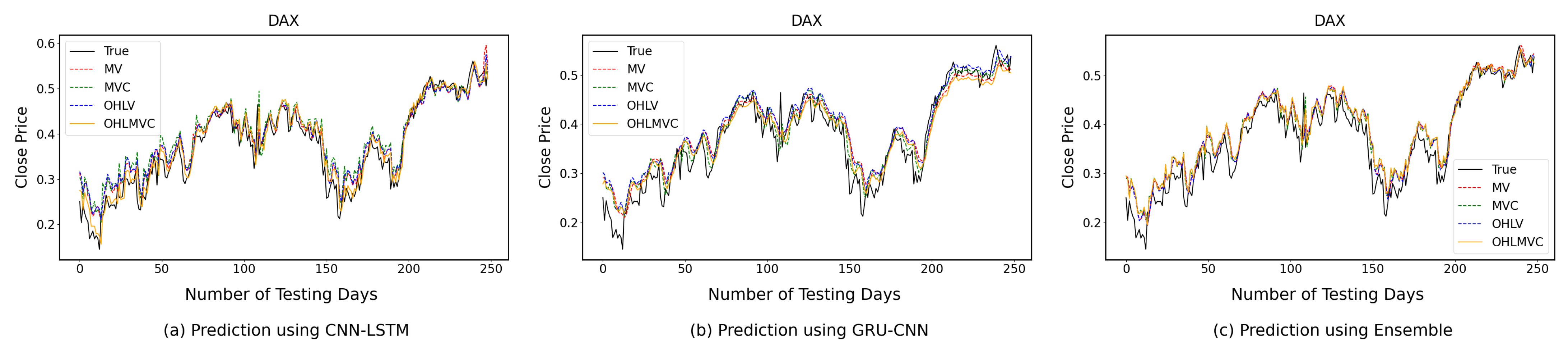
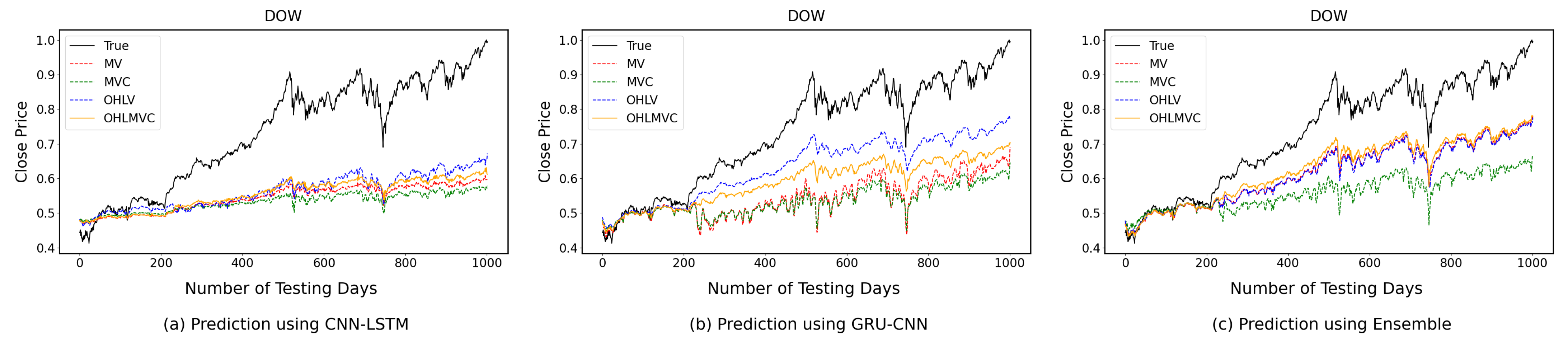
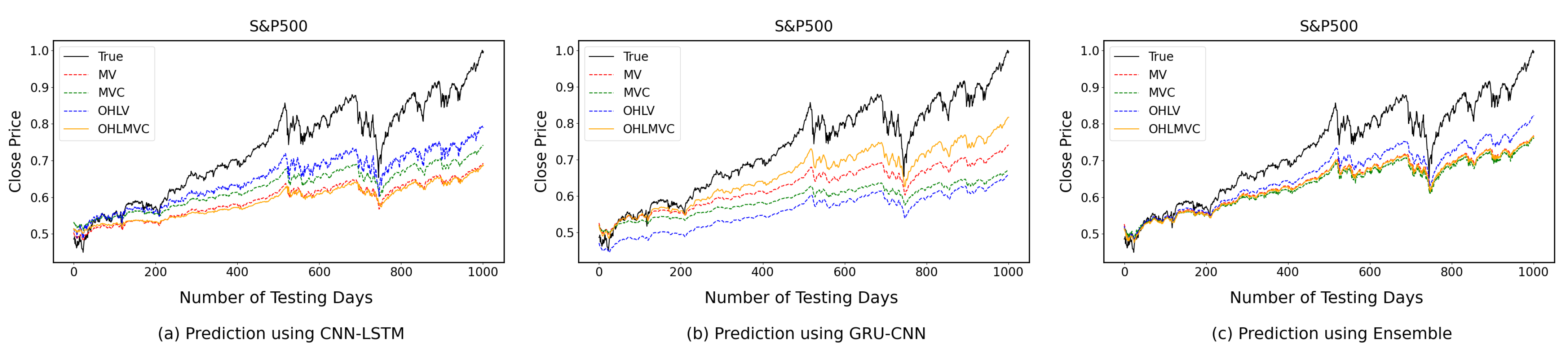
• Novel RNN-based hybrid models are proposed to forecast one-time-step and multi-time-step closing prices of the DAX, DOW, and S&P500 indices by utilizing neural network structures: CNN-LSTM, GRU-CNN, and ensemble models.
• The novel feature, which is the average of the high and low prices of stock market indices, is used as an input feature.
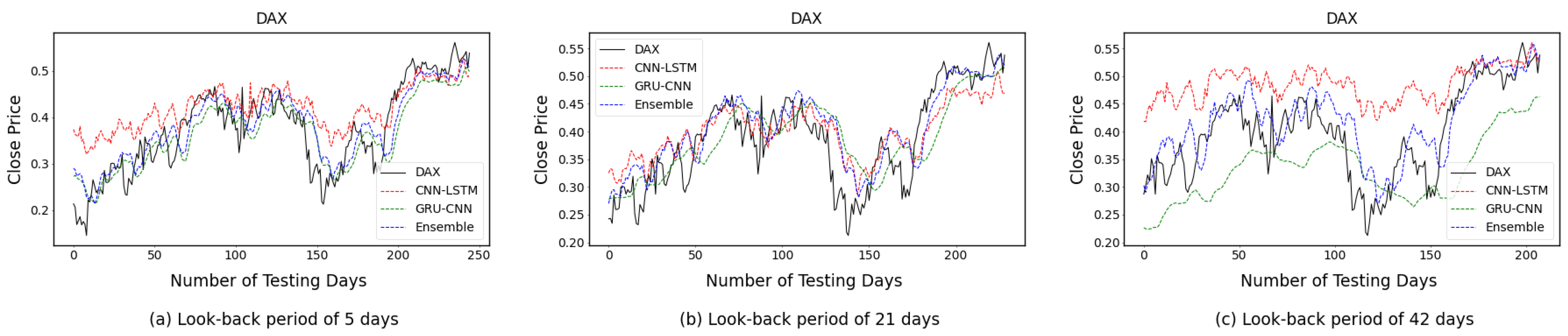
• Comparisons between the proposed and traditional benchmark models with various look-back periods and features are presented.
• The experimental results indicate that the proposed models outperform the benchmark models in 48.1% and 40.7% of the cases in terms of the mean squared error (MSE) and mean absolute error (MAE), respectively, in the case of one-time-step forecasting and 81.5% of the cases in terms of the MSE and MAE in the case of multi-time-step forecasting.
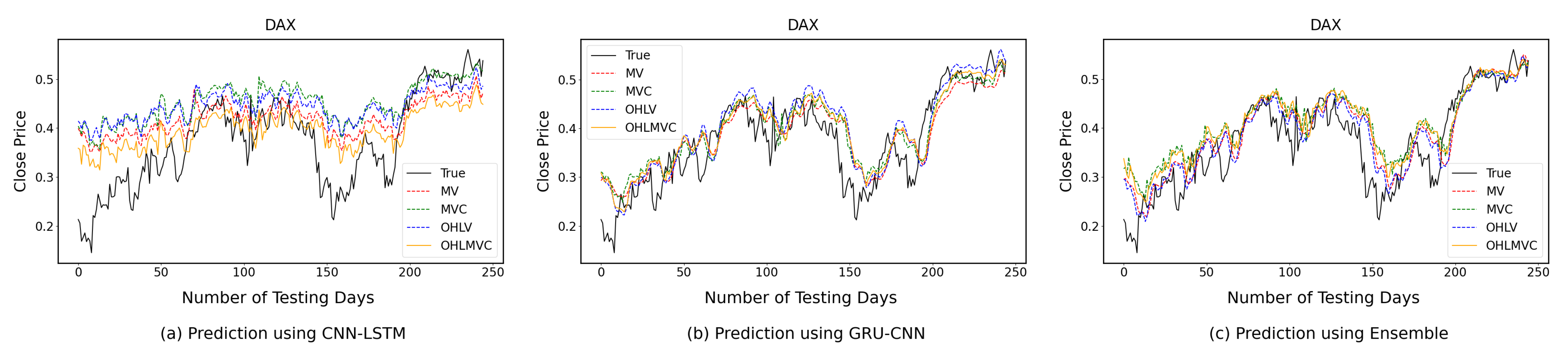
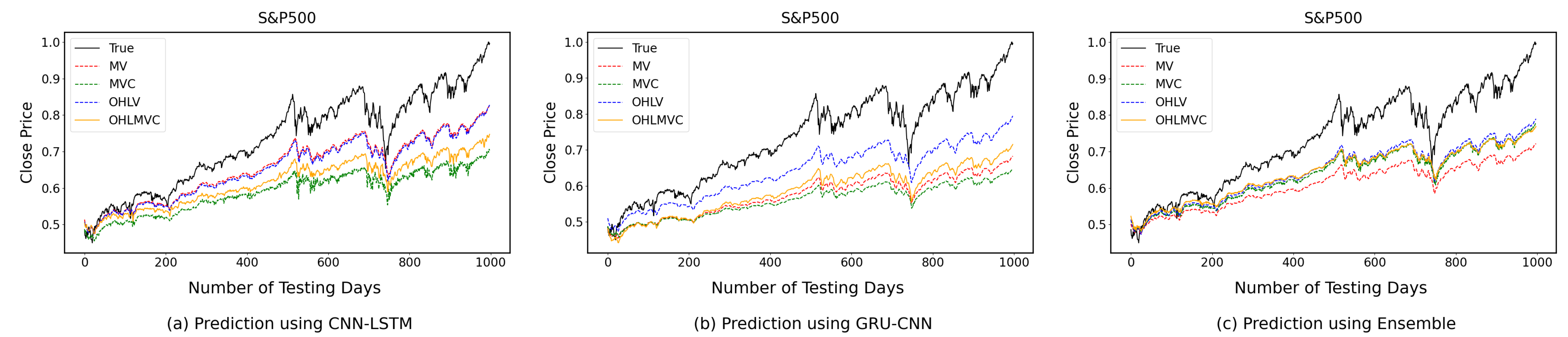
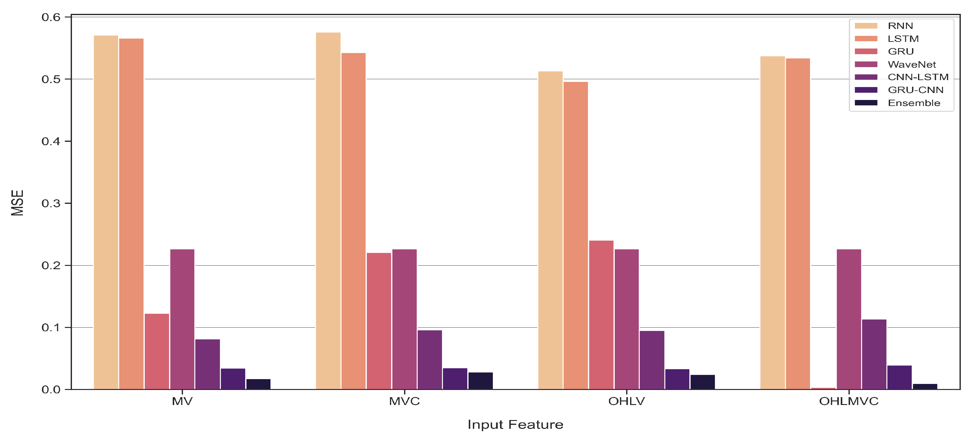
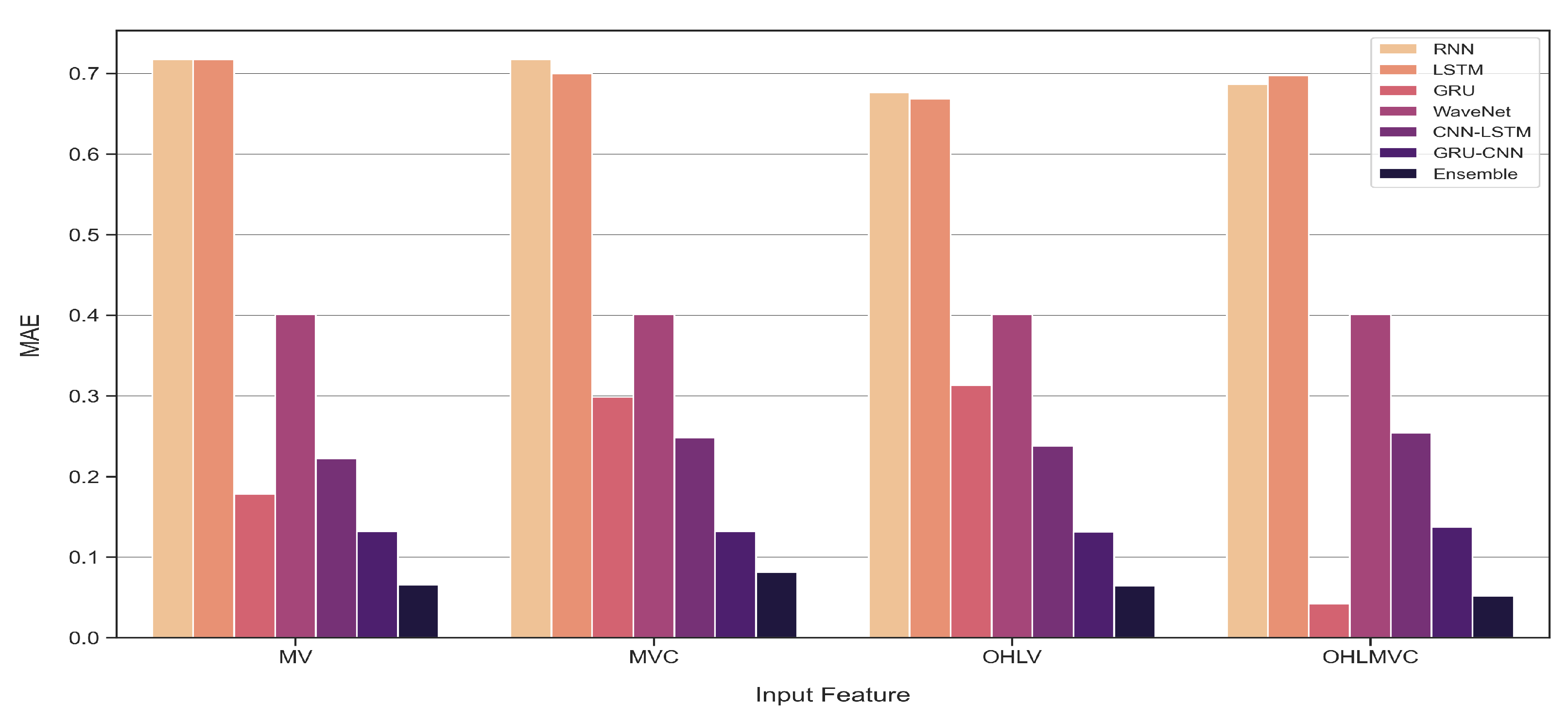
• Further, compared with previous studies that involved using open, high, and low prices, and trading volume of stock market indices as features, in this study, we evaluate the performance of our models by adding a novel feature to reduce the influence of the highest and lowest prices. The results confirm that the newly proposed feature contributes to improving the performance of the models in forecasting stock market indices.
• In particular, the ensemble model provides significant results for one-time-step forecasting.

The remainder of this paper is organized as follows. Section 2 presents an overview of deep learning models and reviews the relevant existing literature on stock market forecasting. Section 3 describes the proposed models designed using RNN-based hybrid architectures and provides the implementation details of the experiment, including the data and experimental setting. In Section 4, we present the experimental results, where we evaluate the proposed models on three stock market indices, compare them with benchmark models, and analyze the effect of the novel feature. Section 5 discusses the implications and advantages of the proposed models. Finally, Section 6 summarizes the conclusions of the study.

2. Background and Related Work

2.1. Deep-Learning Background

In this subsection, we review the artificial neural network (ANN), multilayer perceptron (MLP), CNN, RNN, LSTM, and GRU.

2.1.1. ANN

ANNs, also known as feedforward neural networks, are computing systems inspired by the biological human brain and consist of input, hidden, and output layers with connected neurons, wherein connections between neurons do not form a cycle. An ANN is capable of learning nonlinear functions and processing information in parallel [14]. Each neuron computes the weighted sum of all of its inputs, and a nonlinear activation function is applied to this sum to produce the output result of each neuron. The weights are adjusted to minimize a metric of the difference between the actual and predicted values of the data using the back-propagation algorithm [15].

2.1.2. MLP

The perceptron was proposed by [16] in 1943, representing an algorithm for the supervised learning of binary classifiers. As a linear classifier, a single-layer perceptron is the simplest feedforward neural network. Minsky and Papert [17] showed that a single-layer perceptron is incapable of learning the exclusive or (XOR) problem, whereas an MLP is capable of solving the XOR problem.

An MLP is a fully connected class of ANN. Attempts to solve linearly inseparable problems, such as the XOR problem, have led to different variations in the number of layers and neurons as well as nonlinear activation functions, such as a logistic sigmoid function or a hyperbolic tangent function [18].

2.1.3. CNN

The CNN was proposed to automatically learn spatial hierarchies of features in tasks, such as image recognition and speech recognition [19], by exploiting the spatial relationships among the pixels in an image. In [20], a CNN is composed of convolutional layers, pooling layers, and fully connected layers, and is trained with the adaptive moment estimation (Adam) optimizer on mini batches [21]. The convolutional layers extract the useful features, while the pooling layers reduce the dimensions of the feature maps. The rectified linear unit (ReLU) is applied as a nonlinear activation function [22], and a dropout layer is used as a regularization method in which the output of each hidden neuron is set to zero with a given probability [23].

2.1.4. RNN

The assumption of a traditional neural network is that all the inputs are independent of each other, which makes them ineffective when dealing with sequential data and varied sizes of inputs and outputs [24]. The RNN is an extension of the conventional feedforward neural network and is well suited to sequential data, such as time series, gene sequences, and weather data.

An RNN has memory loops and handles a variable length of input sequence by having a recurrent hidden state [25]. It is known to have a shortcoming of a significant decrease in learning ability as the gradient gradually decreases during back-propagation when the distance between the relevant information and the point is long, which is called the vanishing gradient problem [26]. Errors from later time steps are difficult to propagate back to previous time steps, which results in difficulty in training deep RNNs to preserve information over multiple time steps because the gradients tend to either vanish or explode as they cycle through feedback loops [27]. To address this problem, Hochreiter and Schmidhuber [26] proposed the LSTM, which is capable of solving the vanishing gradient problem using memory cells.

2.1.5. LSTM

The LSTM was proposed by [26] as a variant of the vanilla RNN to overcome the vanishing or exploding gradient problem by adding the cell state to the hidden state of an RNN. The LSTM is composed of a cell state and three gates: input, output, and forget gates. The following equations describe the LSTM architecture.

The forget gate ${\mathbf{f}}_t$ determines which information is input to forget or keep from the previous cell state ${\mathbf{C}}_{t-1}$ and is computed as

$${\mathbf{f}}_t=\sigma ({\mathbf{W}}_{\mathbf{f}}·[{\mathbf{h}}_{t-1},{\mathbf{x}}_t]+{\mathbf{b}}_{\mathbf{f}}),$$

(1)

where ${\mathbf{x}}_t$ is the input vector at time t the function $\sigma$ is a logistic sigmoid function.

The input gate ${\mathbf{i}}_t$ determines which information is updated to the cell state ${\mathbf{C}}_t$ and is computed by

$${\mathbf{i}}_t=\sigma ({\mathbf{W}}_{\mathbf{i}}·[{\mathbf{h}}_{t-1},{\mathbf{x}}_t]+{\mathbf{b}}_{\mathbf{i}}).$$

(2)

The candidate value ${\tilde{\mathbf{C}}}_t$ that can be added to the state is created by a tanh activation function and is computed by

$${\tilde{\mathbf{C}}}_{\mathbf{t}}=tanh({\mathbf{W}}_{\mathbf{C}}·[{\mathbf{h}}_{t-1},{\mathbf{x}}_t]+{\mathbf{b}}_{\mathbf{C}}).$$

(3)

The cell state ${\mathbf{C}}_t$ can store information over long periods of time by updating the internal state and is computed by

$${\mathbf{C}}_t={\mathbf{f}}_t\odot {\mathbf{C}}_{t-1}+{\mathbf{i}}_t\odot {\tilde{\mathbf{C}}}_t,$$

(4)

where the operator ⊙ represents the element-wise Hadamard product.

The output gate ${\mathbf{o}}_t$ determines what information from the cell state to be used as an output by taking the logistic sigmoid activation function, and is computed by

$${\mathbf{o}}_t=\sigma ({\mathbf{W}}_{\mathbf{o}}·[{\mathbf{h}}_{t-1},{\mathbf{x}}_t]+{\mathbf{b}}_{\mathbf{o}}),$$

(5)

and the output ${\mathbf{h}}_t$ is computed as

$${\mathbf{h}}_t={\mathbf{o}}_t\odot tanh\left({\mathbf{C}}_t\right),$$

(6)

where ${\mathbf{W}}_{*}$ and ${\mathbf{b}}_{*}$ represent weight matrices and bias vectors, respectively.

Following [26], the gates decide which information to be forgotten or to be remembered; therefore, the LSTM is suitable for managing long-term dependencies and forecasting time series with different numbers of time steps. Further, it can generalize and handle noise, distributed representations, and continuous values well.

2.1.6. GRU

The GRU, proposed in [28], is a simpler variation of LSTM and has fewer parameters than LSTM. The LSTM has update, input, forget, and output gates and maintains the internal memory state, whereas the GRU has only update and reset gates. It combines the forget and input gates of LSTM into a single update gate and has fewer tensor operations, resulting in faster training than LSTM.

The GRU merges the cell and hidden states. It performs well in sequence learning tasks and overcomes the problems of vanishing or exploding gradients in vanilla RNNs when learning long-term dependencies [29]. It also tends to perform better than LSTM on fewer training data, whereas LSTM is more efficient in remembering longer sequences [30,31,32]. The following equations describe how memory cells at each hidden layer are updated at each time step [33]. The reset gate ${\mathbf{r}}_t$ controls the influence of ${\mathbf{h}}_{t-1}$ and is computed as

$${\mathbf{r}}_t=\sigma \left({\mathbf{W}}_{\mathbf{r}}·[{\mathbf{h}}_{t-1},{\mathbf{x}}_t]\right),$$

(7)

where ${\mathbf{x}}_t$ and ${\mathbf{h}}_{t-1}$ are the input and the previous hidden state, respectively.

The update gate ${\mathbf{z}}_t$ specifies whether to ignore the current information ${\mathbf{x}}_t$ and is computed as

$${\mathbf{z}}_t=\sigma \left({\mathbf{W}}_{\mathbf{z}}·[{\mathbf{h}}_{t-1},{\mathbf{x}}_t]\right).$$

(8)

The computation of candidate activation ${\mathbf{h}}_t$ is similar to that of the traditional recurrent unit, that is,

$${\mathbf{h}}_t={\mathbf{z}}_t\odot {\mathbf{h}}_{t-1}+(1-{\mathbf{z}}_t)\odot {\tilde{\mathbf{h}}}_t,$$

(9)

where

$${\tilde{\mathbf{h}}}_t=tanh\left({\mathbf{W}}_{\mathbf{h}}·[{\mathbf{r}}_t\odot {\mathbf{h}}_{t-1},{\mathbf{x}}_t]\right),$$

(10)

${\mathbf{W}}_{\mathbf{r}}$, ${\mathbf{W}}_{\mathbf{z}}$ and ${\mathbf{W}}_{\mathbf{h}}$ are weight matrices which are learned.

2.2. Related Work

A stock market index is an important indicator of changes in the share prices of different companies, thus informing investment decisions. It is also more advantageous to invest in an index fund than to invest in individual stocks because it keeps costs low and removes the need to constantly manage reports from many companies. However, stock market index forecasting is extremely challenging because of the multiple factors affecting the stock market, such as politics, global economic conditions, unexpected events, and the financial performance of companies listed on the stock market.

Recently, deep-learning models have been extensively applied to numerous areas in finance, such as the forecasting future prices of stocks, prediction of stock price movements, portfolio management, risk assessment, and trading strategies [34,35,36,37,38,39]. Using deep learning-based models, such as CNNs, RNNs, LSTMs, and GRUs, studies have shown that such models outperform classical methods for time series forecasting tasks because of their ability to handle nonlinearity [19,25,26,33].

CNN models have been used in different time series forecasting applications. Chen et al. [40] and Sezer and Ozbayoglu [41] transformed time-series data into two-dimensional image data and used them as inputs for a CNN to classify the movement of the data. Meanwhile, Gross et al. [42] interpreted multivariate time series as space-time pictures.

RNN-based models have been used to predict time-series data. Fischer and Krauss [43] showed that LSTM outperformed memory-free classification methods, such as random forests, deep ANNs, and logistic regression classifiers, in prediction tasks. Dutta et al. [44] proposed the GRU model with recurrent dropout to predict the daily cryptocurrency prices.

Other deep learning models have been applied for time series forecasting. Heaton et al. [45] stacked autoencoders to predict and classify stock prices and their movements. Abrishami et al. [7] used a variational autoencoder to remove noise from the data and stacked LSTM to predict the close price of stocks. Wang et al. [2] used wavelet transform to forecast time-series data.

Moreover, various architectures combining deep learning-based models have been proposed in the literature. Ilyas et al. [46] combined technical and content features via learning time series and textual data, Livieris et al. [47] introduced the CNN-LSTM model to predict gold prices and movements, while Daradkeh [6] integrated a CNN and a bidirectional LSTM to predict stock trends. Zhang et al. [4] combined attention and LSTM models for financial time series prediction. Livieris and Pintelas [48] proposed ensemble learning strategies with advanced deep learning models for forecasting cryptocurrency prices and movements. Bao et al. [24] combined wavelet transforms, stacked autoencoders, and LSTM to forecast the closing stock prices for the next day by eliminating noise from the data and generating deep high-level features. Meanwhile, Zhang et al. [49] proposed a novel architecture of a generative adversarial network (GAN) with an MLP as the discriminator and an LSTM as the generator for forecasting the closing price of stocks.

Further, Leung et al. [50] proposed a two-timescale duplex neurodynamic approach for solving the portfolio optimization problem, and several studies have applied an LSTM to construct a portfolio [36,51,52,53,54,55].

This study proposes three models by combining CNN and RNN-based models for predicting the stock market index. Additionally, in contrast to existing studies, which employed open, high, and low prices, trading volume, and change in stock market indices, we introduce a novel input feature: the average of high and low prices. Furthermore, the three proposed models are evaluated on three daily stock market indices with two different optimizers and four different features. Finally, we compare the performance of the proposed models with conventional benchmark models with respect to forecasting the closing prices of the stock market indices.

3. Materials and Methods

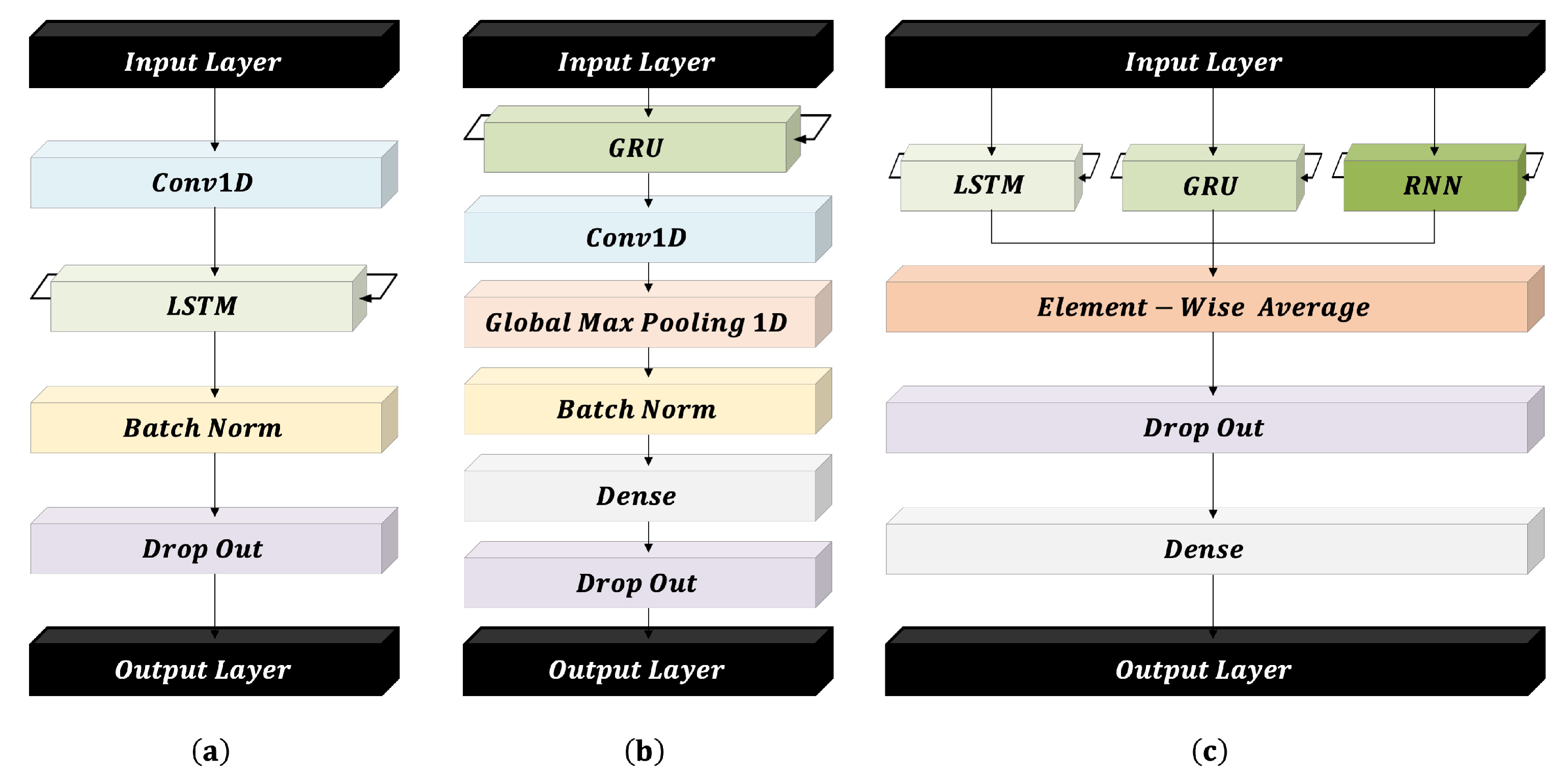
3.1. Proposed Models

Following Livieris and Pintelas [48], by combining prediction models, a bias is added, which in turn reduces the variance, resulting in a better performance than that of single models. Therefore, we propose three RNN-based hybrid models that predict the stock market indices for one-time-step and multi-time-step at a time.

3.1.1. Proposed CNN-LSTM Model

CNNs can effectively learn the internal representations of time-series data [47]. The one-dimensional convolutional layer filters out the noise, extracts spatial features, and reduces the number of parameters. The causal convolution ensures that the output at time t derives only inputs from time $t-1$. RNNs are considered the best sequential deep-learning models for forecasting time-series data. To this end, we combine a one-dimensional CNN and an LSTM in a new model: CNN-LSTM. The CNN-LSTM model consists of (1) a one-dimensional convolutional layer, (2) an LSTM layer, (3) a batch-normalization layer, (4) a dropout layer, and (5) a dense layer.

To determine the best-performing parameters, we examined different variants of the model: the number of hidden layers (1 and 2), the number of neurons (64 and 128), the batch size (32 and 64), and the dropout rate ($0.2$ and $0.5$).

The best-performing CNN-LSTM model comprised a one-dimensional convolutional layer with 32 filters of size 3 with a stride of 1, causal padding, and the ReLU activation function; an LSTM layer with 128 units and tanh activation function; a batch-normalization layer; a dropout layer with a rate of $0.2$; and a dense layer with a prediction window size of units and the ReLU activation function. Figure 1 illustrates the architecture of the proposed CNN-LSTM model, while

Table 1. Model configuration of the proposed models.

Model	Description
CNN-LSTM	One-dimensional convolutional layer with 32 filters of size 3 with a stride of 1
	LSTM layer with 128 units and tanh activation function
	Batch-normalization layer
	Dropout layer with a rate of 0.2
	Dense layer with a prediction window size of units
GRU-CNN	GRU layer with 128 units and the tanh activation
	One-dimensional convolutional layer with 32 filters of size 3 with a stride of 1
	One-dimensional global max-pooling layer
	Batch-normalization layer
	Dense layer with 10 units and the ReLU activation
	Dropout layer with a rate of 0.2
	Dense layer with a prediction window size of units
Ensemble	RNN layer with 128 units and the tanh activation function
	LSTM layer with 128 units and the tanh activation function
	GRU layer with 128 units and the tanh activation function
	Average of all the hidden states from RNN, LSTM, and GRU
	Dropout layer with a rate of 0.2
	Dense layer with 32 units and the ReLU activation function
	Dense layer with a prediction window size of units

summarizes the configuration.

3.1.2. Proposed GRU-CNN Model

The GRU is simpler than LSTM, has the ability to train sequential patterns, and takes less time to train the model with improved network performance. To utilize both GRU and one-dimensional CNN, we propose a stacked architecture where a GRU and a one-dimensional CNN are combined, namely the GRU-CNN model. The parameters used for the GRU-CNN model were similar to those of the CNN-LSTM model, as described in Section 3.1.1. The difference between the CNN-LSTM and GRU-CNN models is in the order of stacking the RNN and CNN layers.

The GRU-CNN model consists of a GRU layer with 128 units and the tanh activation function; a one-dimensional convolutional layer with 32 filters of size 3 with a stride of 1, causal padding, and the ReLU activation function; a one-dimensional global max-pooling layer; a batch-normalization layer; a dense layer with 10 units and the ReLU activation function; a dropout layer with a rate of $0.2$; and a dense layer with a prediction window size of units and the ReLU activation function. In the GRU-CNN model, the GRU layer returns a sequence, and the one-dimensional global max-pooling layer takes only important features and reduces the dimension of the feature map. The architecture of the proposed GRU-CNN model is illustrated in Figure 1, while the configuration is listed in Table 1.

3.1.3. Proposed Ensemble Model

While evaluating the performance of the benchmark models, various RNN models, such as RNN, LSTM, and GRU, exhibited high predictive performance on different types of datasets. There are three types of widely employed ensemble learning strategies: ensemble averaging, bagging, and stacking. Based on the results of the benchmarks, the CNN-LSTM, and the GRU-CNN as implemented above, we propose an average ensemble of three RNN-based models to achieve averaged high performance for various datasets. The proposed ensemble model can utilize the representations of the RNN, LSTM, and GRU models. The parameters used for the ensemble model were similar to those of the CNN-LSTM and GRU-CNN models, as described in Section 3.1.1.

The ensemble model consists of an RNN layer with 128 units and the tanh activation function; an LSTM layer with 128 units and the tanh activation function; a GRU layer with 128 units and the tanh activation function; followed by taking the average of all the hidden states from RNN, LSTM, and GRU; a dropout layer with a rate of $0.2$; a dense layer with 32 units and the ReLU activation function; and a dense layer with a prediction window size of units and the ReLU activation function. Figure 1 illustrates the details of each layer of the proposed ensemble model, while Table 1 presents the configuration.

3.2. Implementation Details

In this subsection, we present an extensive empirical analysis of the proposed models on three datasets. First, we describe the datasets and the experimental setting used to demonstrate the validity of our financial time-series prediction models. Next, we evaluate the performance of our models on several datasets and compare them with those of conventional deep learning models.

3.2.1. Dataset

We evaluated the performance of the proposed models on daily stock market indices to verify the robustness of our models. We considered three stock market indices from major stock markets listed below.

(1)

DAX: Deutscher Aktienindex, which is a stock market index consisting of the 40 (expanded from 30 in 2021) major German blue-chip companies trading on the Frankfurt stock exchange.

(2)

DOW: Dow Jones Industrial Average, which is a stock market index of 30 prominent companies in the United States.

(3)

S&P500: Standard and Poor’s 500, which is a stock market index of 500 large companies in the United States.

The DOW is the most influential and widely used stock market index in the literature. We considered three types of periods for all three indices: the period from 1 January 2000 through 31 December 2019 for DOW and S&P500 and from 24 October 2014 through 31 December 2019 for DAX as long periods; from 1 January 2017 through 31 December 2019 and from 1 January 2019 through 31 December 2021 as short periods before and after the COVID-19 pandemic, respectively.

The historical prices of each stock market index were obtained using the FinanceDataReader open-source library available in the pandas $DataReader$ module of the Python programming language [56]. The raw data included six features: open, high, low, and close prices, trading volume, and change. The incomplete data were removed.

Before feeding the raw data into our models, we pre-processed the data. We normalized the raw data using Scikit-learn’s $MinMaxScaler$ tool, as follows:

$$x=\frac{x-x_{max}}{x_{max}-x_{min}},$$

(11)

where x is the input feature of the stock market index and $x_{max}$ and $x_{min}$ are the maximum and minimum values of each input feature, respectively. Granger [57] suggested holding approximately $20\%$ of the data for out-of-sample testing. Following this suggestion, the first $80\%$ of the data were used as the training set for in-sample training, while the remaining $20\%$ were used as the test set, to ensure that our models were evaluated on unseen out-of-sample data. The first $90\%$ of the training set was used to train the network and to iteratively adjust its parameters such that the loss function was minimized. The trained network predicted the remaining $10\%$ for validation, and the validation loss was computed after each epoch.

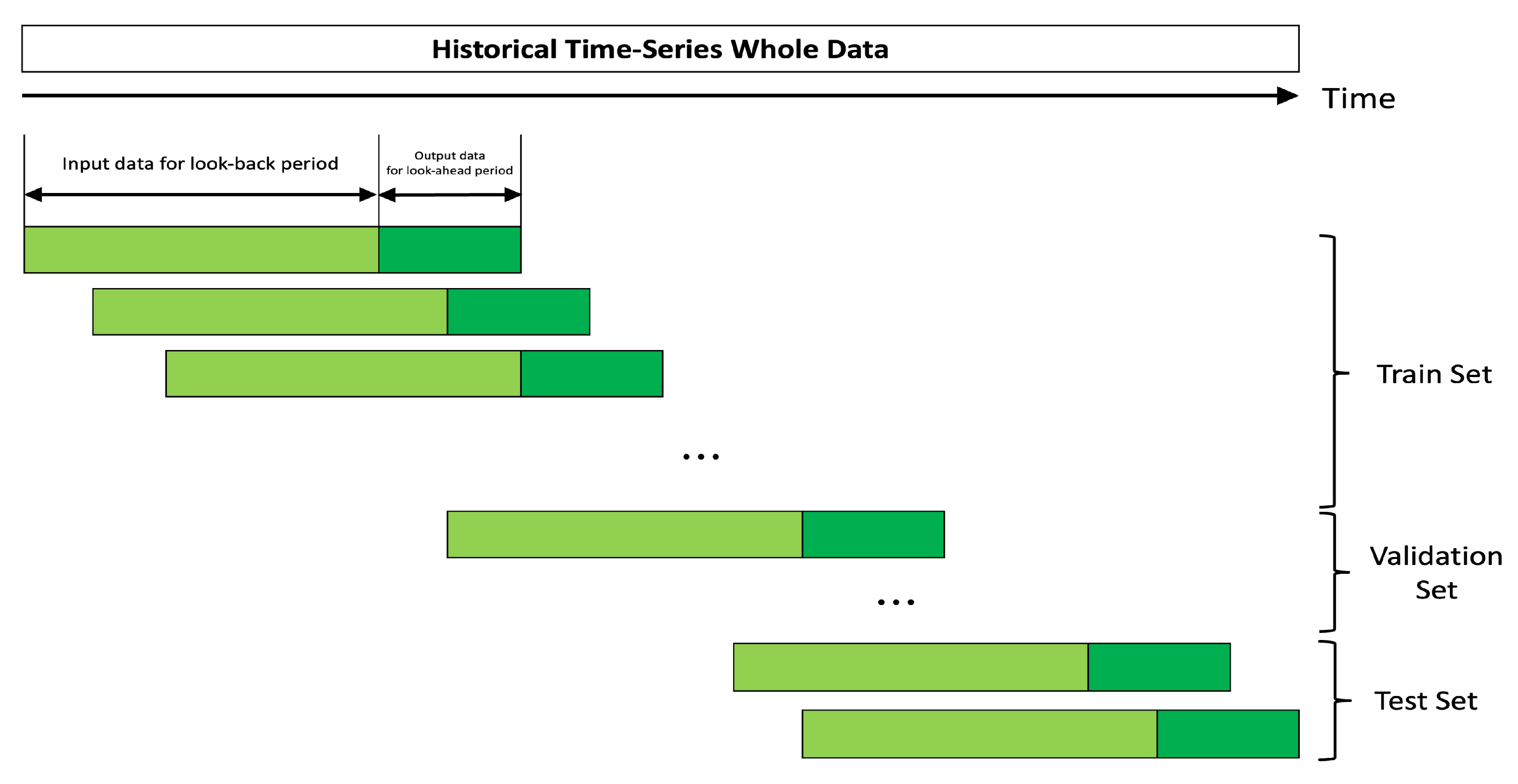
3.2.2. Generation of the Inputs and Outputs Using the Sliding Window Technique

This subsection describes the generation of the inputs and outputs. The daily open, high, and low prices, trading volume, and change were commonly used as input features in other studies. However, in the current study, we introduce a novel feature named medium, which is the average of high and low prices, to reduce the influence of the unusually extreme highest and lowest prices and to ensure generalizability.

For each stock market index, the partial features of daily open, high, low, and medium prices, trading volume, and change (OHLMVC) were used as the input to train the model, and the daily close prices were used as the output to predict one-time-step and multi-time-step ahead.

For the input and output generation, the normalized data were segmented using the sliding window technique, by which a fixed window size of time-series data was chosen as the input and a fixed number of the following observations was chosen as the output. This process was repeated for the entire dataset by sliding the window in intervals of one time step to obtain the next input and output. We trained the proposed models to look at m consecutive past data of features. The input at time t was denoted by

$${\mathbf{X}}_t=\left({\mathbf{x}}_t^O,{\mathbf{x}}_t^H,{\mathbf{x}}_t^L,{\mathbf{x}}_t^M,{\mathbf{x}}_t^V,{\mathbf{x}}_t^{Ch}\right)\in {\mathbb{R}}^{m\times 6},$$

(12)

where for each $k\in \{O,H,L,M,V,Ch\}$,

$${\mathbf{x}}_t^k={\left(x_{t-m+1}^k,\cdots ,x_{t-1}^k,x_t^k\right)}^T\in {\mathbb{R}}^m,$$

(13)

${\mathbf{x}}^O,{\mathbf{x}}^H,{\mathbf{x}}^L,{\mathbf{x}}^M,{\mathbf{x}}^V,$ and ${\mathbf{x}}^{Ch}$ are the daily open, high, low, and medium prices, trading volume, and change from time $t-m+1$ to time t, respectively.

The input ${\mathbf{X}}_t$ was fed sequentially into the proposed models to predict the following n daily close prices of stock market indices, with the output denoted by

$${\mathbf{y}}_{t+1}^C={\left(y_{t+1},y_{t+2},...y_{t+n}\right)}^T\in {\mathbb{R}}^n.$$

(14)

The look-back periods of $5,21$, and 42 days were considered as one week, one month, and two months, respectively; while the look-ahead periods of one and five days were considered to predict the future one-time-step or multi-time-step ahead. Figure 2 illustrates the sliding window technique.

3.2.3. Software and Hardware

The proposed models were implemented, trained, and analyzed in Python $3.7.6$ [58] with the Keras library $2.4.3$ [59] as a high-level neural network API using TensorFlow $2.3.1$ as back-end [60], relying on NumPy $1.19.2$[61], Pandas $0.25.3$[56], and Scikit-learn $1.0.2$ [62]. The code used for producing the figures and analysis is available on GitHub at https://github.com/hyunsunsong/Project (accessed on 27 March 2023).

All experiments were performed using a workstation equipped with an Intel Xeon Silver 4208 CPU at 2.10 GHz x8, Nvidia GPU TITAN, and 12 GB RAM on each board.

3.2.4. Experimental Setting

The proposed models were trained with the Huber loss function, which combines the characteristics of MSE and MAE and is less susceptible to outliers in the data than the MSE loss function [63]. It behaves quadratically for small residuals and linearly for large residuals [64]. The parameters of the network were learned to minimize the average of the Huber loss function over the entire training dataset.

The network weights and biases were initialized with the Glorot–Xavier uniform method and zeros, respectively. Glorot and Bengio [65] proposed the Glorot–Xavier uniform method to adopt a properly scaled uniform distribution for initialization.

The successful applications of neural networks require regularization [66]. Introduced by [23], the dropout regularization technique randomly drops a fraction of the units with a specified probability, along with connections during training, while all units are presented during testing. We applied the dropout values of $0.2$ and $0.5$ to reduce overfitting and have observed that higher dropout value result in a decline in performance. Therefore, we settled on the relatively low dropout value of $0.2$ as studied in [67].

The batch size and maximum number of epochs were set to 32 and 50, respectively, and an early stopping patience of 10 was applied [68]. That is, once the validation loss no longer decreased for the patience period, the training was stopped, and the weights of the model with the lowest validation loss were restored using ModelCheckpoint callback in the Keras library [59].

The optimization algorithms used for training were the Adam and root mean square propagation (RMSProp) [69], which are adaptive learning rate methods. The RMSProp is usually a viable choice for RNNs [59]. We compared the performance of the proposed models using two different optimizers.

We applied learning rates of $0.001$ and $0.0005$ and found that a learning rate of $0.0005$ resulted in a better performance. Therefore, the learning rate was set to $0.0005$.

The ReLU activation function proposed in [22] was used for the dense layers, and the data shuffling technique was not used during training.

3.2.5. Predictive Performance Metrics

In this study, we adopted the MSE and MAE as evaluation metrics to compare the performance of the proposed models with that of conventional benchmark models for forecasting time-series data, which are calculated as follows:

$$\mathrm{MSE}=T\sum _{t=1}^T{\left(y_t-\widehat{y_t}\right)}^2,$$

(15)

$$\mathrm{MAE}=T\sum _{t=1}^T\left|y_t-\widehat{y_t}\right|,$$

(16)

where T is the number of prediction time horizons; $y_t$ and $\widehat{y_t}$ are the true and predicted values, respectively, during one-time-step prediction. During multi-time-step prediction, we only used the value of the last time step; thus, $y_t$ and $\widehat{y_t}$ represent the true and predicted values of the last time step, respectively.

4. Experimental Results

In this section, we present the experimental results of the proposed models using historical time-series data for three stock market indices: DAX, DOW, and S&P500. We first describe the details of the benchmark models used for comparison. Second, we compare the results for the proposed models and conventional benchmarks with respect to one-time-step and multi-time-step predictions on three datasets over three different periods. Third, we present the results of the impact of different features and optimizers on the performance of the proposed models.

4.1. Benchmark Models

For benchmark comparison, we deploy several conventional deep learning models, such as RNN, LSTM, and GRU, to examine whether the proposed models outperform the benchmarks. In addition, we utilize WaveNet, which combines causal filters with dilated convolutions, so that the model learns long-range temporal dependencies in time-series data [70]. The benchmark models and corresponding architectures are listed below.

• RNN: Two RNN layers with 128 units and a dense layer with a look-ahead period of units;
• LSTM: An LSTM layer with 128 units and a dense layer with a look-ahead period of units;
• GRU: A GRU layer with 128 units and a dense layer with a look-ahead period of units;
• WaveNet: A simpler architecture of an audio generative model based on PixelCNN [71], as described in [70].

Table 2. Hyperparameter setting for the benchmark models.

Hyperparameter	Value
Number of epochs	50
Early stopping patience	10
Learning rate	0.0005
Batch size	32
Loss function	MSE
Optimizer	Adam
Activation function	ReLU

lists the training setting for the benchmark models. All benchmark models were trained with 50 epochs, an early stopping patience of 10, a learning rate of $0.0005$, a batch size of 32, the MSE loss function, the Adam optimizer, and the ReLU activation function.

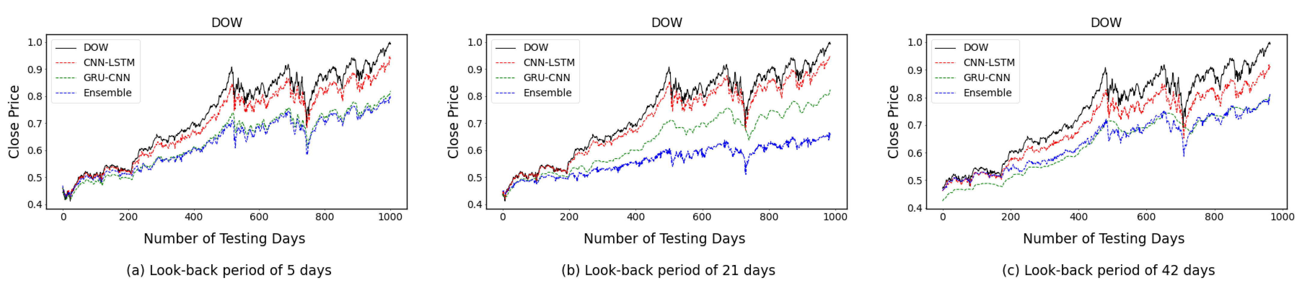
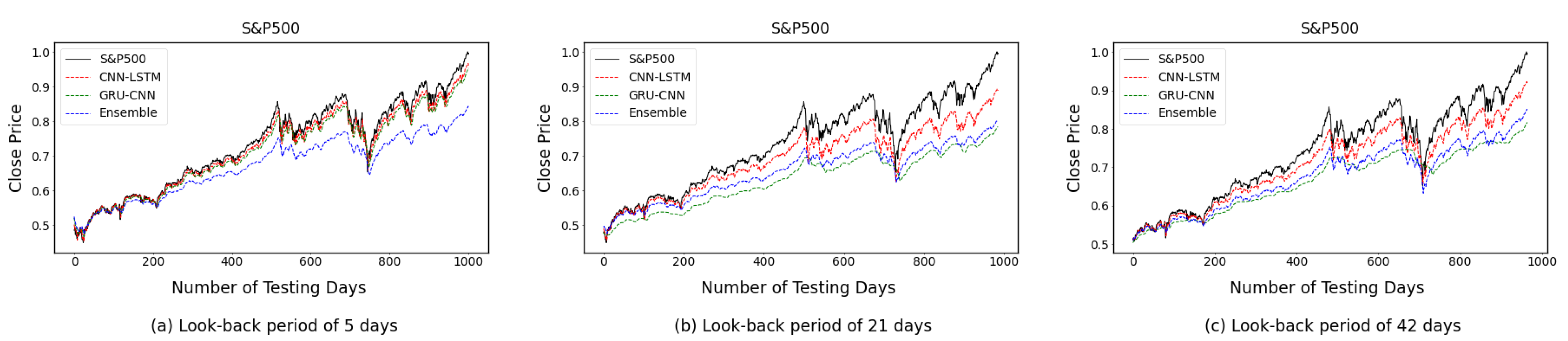
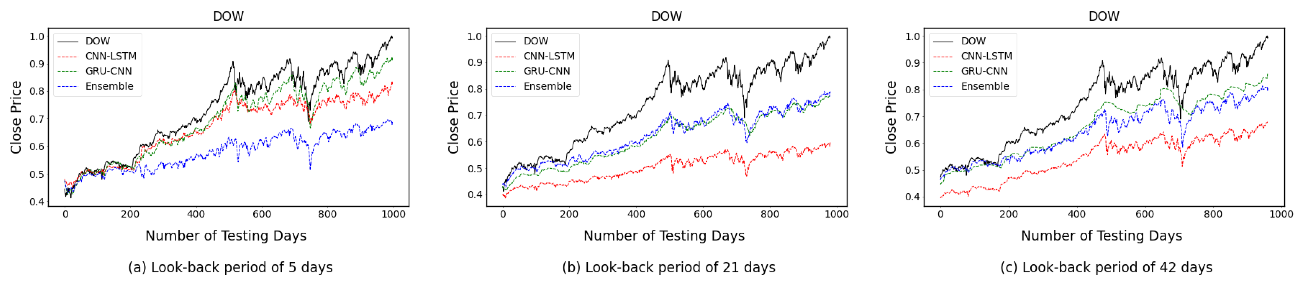
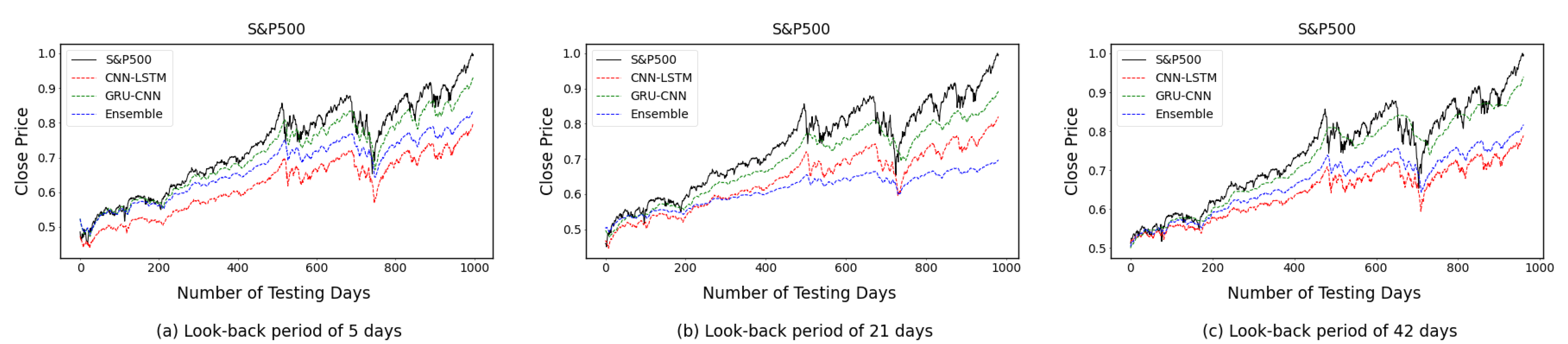
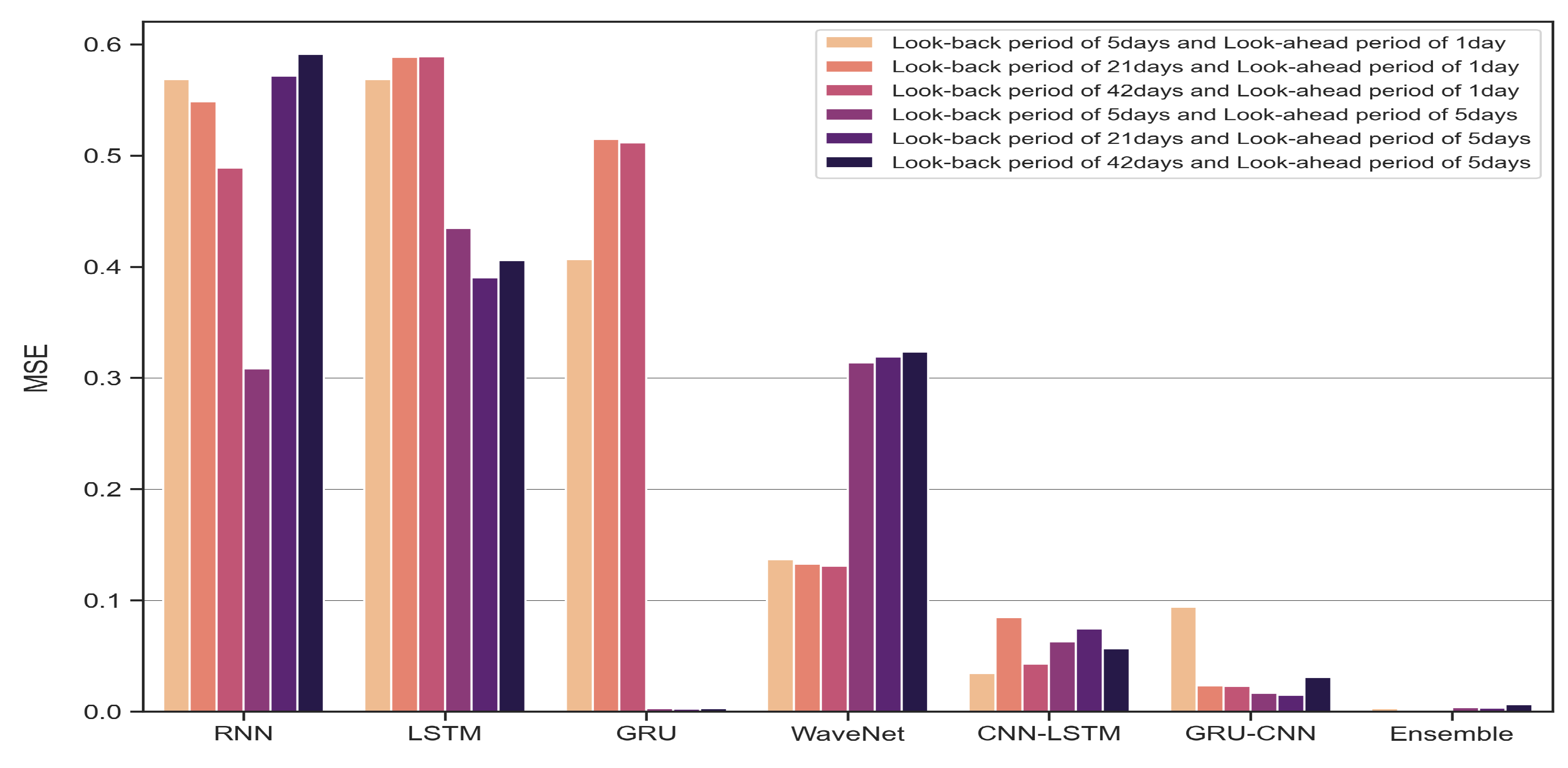
4.2. One-Time-Step Prediction Comparisons between Proposed and Benchmark Models

In this subsection, we provide the experimental results of the proposed models to predict the one-time-step ahead of the three stock market indices. We evaluated the performance of the proposed models with various look-back periods of $5,21,$ and 42 days as one week, one month, and two months, respectively, for different periods. The proposed and benchmark models were implemented as described in previous sections. The Adam optimizer and OHLV features were used for all methods in

Table 3. Comparison of one-time-step prediction between proposed and benchmark models.

Look-Back Period	Metric	Model	2000–2019 1				2017–2019				2019–2021
			DAX	DOW	S&P500		DAX	DOW	S&P500		DAX	DOW	S&P500
5 days	MSE	RNN	0.1505	0.5739	0.5618		0.1146	0.6942	0.6174		0.7626	0.8576	0.7843
		LSTM	0.1505	0.5739	0.5618		0.1146	0.6942	0.6174		0.7626	0.8576	0.7843
		GRU	0.1505	0.5739	0.0004		0.0012	0.6942	0.6174		0.7626	0.8576	0.0049
		WaveNet	0.4040	0.0940	0.0886		0.4929	0.0411	0.0672		0.0177	0.0075	0.0189
		CNN-LSTM	0.0079	0.0004	0.0040		0.0539	0.0154	0.1333		0.0868	0.0045	0.0032
		GRU-CNN	0.0011	0.0132	0.0042		0.0014	0.0069	0.0135		0.0111	0.0103	0.7843
		Ensemble	0.0017	0.0075	0.0059		0.0012	0.0023	0.0011		0.0009	0.0029	0.0003
	MAE	RNN	0.3756	0.7410	0.7376		0.3207	0.8282	0.7779		0.8717	0.9253	0.8834
		LSTM	0.3756	0.7410	0.7376		0.3207	0.8282	0.7779		0.8717	0.9253	0.8834
		GRU	0.3756	0.7410	0.0185		0.0273	0.8282	0.7779		0.8717	0.9253	0.0674
		WaveNet	0.6284	0.2645	0.2680		0.6942	0.1841	0.2384		0.1224	0.0781	0.1235
		CNN-LSTM	0.0827	0.0162	0.0600		0.2120	0.1188	0.3520		0.2909	0.0650	0.0544
		GRU-CNN	0.0255	0.1031	0.0593		0.0279	0.0779	0.1113		0.1022	0.0991	0.8834
		Ensemble	0.0336	0.0740	0.0651		0.0262	0.0418	0.0279		0.0244	0.0468	0.0143
21 days	MSE	RNN	0.1509	0.5058	0.5341		0.0982	0.6552	0.6482		0.7252	0.8119	0.8070
		LSTM	0.1658	0.5734	0.5602		0.1066	0.7420	0.6781		0.7555	0.8855	0.8273
		GRU	0.1658	0.5734	0.0002		0.0008	0.7420	0.6781		0.7555	0.8855	0.8273
		WaveNet	0.3877	0.0903	0.0856		0.4931	0.0371	0.0605		0.0196	0.0065	0.0154
		CNN-LSTM	0.0078	0.0159	0.0033		0.0632	0.0148	0.1074		0.1507	0.1950	0.2035
		GRU-CNN	0.0014	0.0356	0.0149		0.1066	0.0170	0.0193		0.0090	0.0033	0.0018
		Ensemble	0.0008	0.0007	0.0014		0.0009	0.0023	0.0011		0.0008	0.0011	0.0004
	MAE	RNN	0.3769	0.6934	0.7188		0.2927	0.8025	0.7941		0.8497	0.8987	0.8959
		LSTM	0.3965	0.7418	0.7375		0.3074	0.8559	0.8145		0.8680	0.9401	0.9074
		GRU	0.3965	0.7418	0.0136		0.0222	0.8559	0.8145		0.8680	0.9401	0.9074
		WaveNet	0.6166	0.2596	0.2639		0.6936	0.1736	0.2251		0.1320	0.0722	0.1120
		CNN-LSTM	0.0742	0.1178	0.0473		0.2296	0.1177	0.3223		0.3865	0.4398	0.4479
		GRU-CNN	0.0290	0.1741	0.1135		0.3074	0.1224	0.1317		0.0888	0.0542	0.0384
		Ensemble	0.0211	0.0220	0.0312		0.0240	0.0426	0.0280		0.0201	0.0281	0.0160
42 days	MSE	RNN	0.1619	0.4885	0.4736		0.1147	0.5921	0.5475		0.5888	0.7551	0.6797
		LSTM	0.1683	0.5904	0.5766		0.1228	0.7307	0.6683		0.7352	0.8806	0.8292
		GRU	0.1683	0.5904	0.0013		0.0009	0.7307	0.6683		0.7352	0.8806	0.8292
		WaveNet	0.3732	0.0856	0.0816		0.5011	0.0378	0.0595		0.0211	0.0058	0.0125
		CNN-LSTM	0.0025	0.0342	0.0210		0.0496	0.0783	0.0392		0.0833	0.0759	0.0004
		GRU-CNN	0.0035	0.0459	0.0220		0.0075	0.0128	0.0128		0.0019	0.0712	0.0270
		Ensemble	0.0007	0.0012	0.0007		0.0015	0.0013	0.0039		0.0009	0.0004	0.0007
	MAE	RNN	0.3940	0.6829	0.6795		0.3161	0.7602	0.7295		0.7644	0.8666	0.8227
		LSTM	0.4013	0.7536	0.7486		0.3282	0.8492	0.8087		0.8561	0.9737	0.9091
		GRU	0.4013	0.7536	0.0343		0.0239	0.8492	0.8087		0.8561	0.9377	0.9091
		WaveNet	0.6053	0.2532	0.2583		0.6978	0.1723	0.2192		0.1372	0.0670	0.1001
		CNN-LSTM	0.0453	0.1844	0.1428		0.1883	0.2781	0.1910		0.2855	0.2738	0.0152
		GRU-CNN	0.0459	0.2004	0.1399		0.0725	0.1021	0.1074		0.0384	0.2652	0.1611
		Ensemble	0.0204	0.0308	0.0224		0.0289	0.0313	0.0548		0.0230	0.0167	0.0217

¹ The period from 24 October 2014 through 31 December 2019 for the DAX.

.

Table 3 compares our models and the benchmark models for the different look-back periods for one-time-step prediction, where the best performance results are marked in bold for each stock market index, period, and metric.

According to the results in Table 3, increasing the look-back period slightly enhances the performance across all operating conditions by keeping all other hyperparameters constant. Moreover, a very long sequence length, such as the look-back period of 42, increases the performance. From 1 January 2000 through 31 December 2019, the proposed models improved the benchmarks in 77.8% and 77.8% of cases in terms of MSE and MAE, respectively. Additionally, our models outperformed the benchmarks in 66.7% and 77.8% of cases in terms of MSE and MAE, respectively, for the period from 1 January 2017 through 31 December 2019, before the COVID-19 pandemic, and in 100% of cases for the period from 1 January 2019 through 31 December 2021, after the COVID-19 pandemic, in terms of both MSE and MAE. Some results were the same for different benchmarks because the training algorithm might find the local optima. Further, an overall comparison between the ensemble model and other models in Table 3 indicates that the ensemble model significantly outperformed the other models.

We evaluated the performance of the proposed models with four different features (i.e., MV, MVC, OHLV, and OHLMVC) in addition to a novel feature, medium, defined as the average of high and low prices. In comparison, OHLVs have been commonly used as features in other studies.

In addition, we evaluated the performance of our models using two different optimizers, Adam and RMSProp, by keeping all other hyperparameters constant. The average MSE and MAE over the three periods for the impact of different features and optimizers of the proposed models are shown in

Table 4. Comparison of different optimizers and features in terms of average MSE over the three periods for one-time-step prediction.

Look-Back Period	Optimizer	Feature	CNN-LSTM				GRU-CNN				Ensemble
			DAX	DOW	S&P500		DAX	DOW	S&P500		DAX	DOW	S&P500
5 days	Adam	MV	0.0406	0.0228	0.0154		0.0025	0.0070	0.2717		0.0014	0.0039	0.0026
		MVC	0.0534	0.0366	0.0097		0.0026	0.0054	0.0053		0.0014	0.0039	0.0026
		OHLV	0.0495	0.0068	0.0468		0.0045	0.0101	0.2674		0.0013	0.0042	0.0025
		OHLMVC	0.0496	0.0025	0.0030		0.0070	0.0096	0.2668		0.0013	0.0042	0.0025
	RMSProp	MV	0.0231	0.0239	0.0189		0.0023	0.0088	0.0063		0.0013	0.0031	0.0014
		MVC	0.0972	0.0796	0.0270		0.0035	0.0197	0.0171		0.0013	0.0031	0.0014
		OHLV	0.0175	0.0133	0.0206		0.0019	0.0144	0.2223		0.0013	0.0031	0.0014
		OHLMVC	0.0330	0.0152	0.0396		0.0043	0.2513	0.0107		0.0013	0.0031	0.0014
21 days	Adam	MV	0.0174	0.0454	0.0217		0.0070	0.0133	0.0180		0.0010	0.0029	0.0011
		MVC	0.1042	0.0489	0.1143		0.0030	0.0141	0.0115		0.0021	0.0040	0.0080
		OHLV	0.0739	0.0752	0.1047		0.0390	0.0186	0.0120		0.0008	0.0013	0.0010
		OHLMVC	0.0406	0.0228	0.0154		0.0054	0.0253	0.0138		0.0021	0.0040	0.0080
	RMSProp	MV	0.0295	0.1721	0.2440		0.0163	0.0183	0.0242		0.0010	0.0042	0.0060
		MVC	0.0318	0.0608	0.1752		0.0395	0.0306	0.0178		0.0017	0.0185	0.0038
		OHLV	0.0477	0.1299	0.3043		0.0157	0.0229	0.0137		0.0008	0.0014	0.0015
		OHLMVC	0.0406	0.0228	0.0154		0.0284	0.0244	0.0253		0.0021	0.0040	0.0080
42 days	Adam	MV	0.0443	0.0790	0.0105		0.0163	0.0169	0.2459		0.0014	0.0028	0.0022
		MVC	0.0566	0.0585	0.0426		0.0227	0.0271	0.2339		0.0010	0.2455	0.0129
		OHLV	0.0451	0.0628	0.0202		0.0043	0.0433	0.0206		0.0010	0.0010	0.0018
		OHLMVC	0.0488	0.1413	0.0102		0.0088	0.0126	0.0124		0.0019	0.0026	0.0012
	RMSProp	MV	0.1339	0.0792	0.1816		0.0084	0.0503	0.0223		0.0017	0.0036	0.0035
		MVC	0.0659	0.2908	0.1823		0.0191	0.0609	0.3112		0.0012	0.0057	0.0049
		OHLV	0.3795	0.3173	0.0588		0.0079	0.0394	0.0341		0.0008	0.0021	0.2784
		OHLMVC	0.0496	0.0607	0.6410		0.0100	0.0256	0.0229		0.0010	0.0021	0.0017

and

Table 5. Comparison of different optimizers and features in terms of average MAE over the three periods for one-time-step prediction.

Look-Back Period	Optimizer	Feature	CNN-LSTM				GRU-CNN				Ensemble
			DAX	DOW	S&P500		DAX	DOW	S&P500		DAX	DOW	S&P500
5 days	Adam	MV	0.1635	0.1285	0.1161		0.0405	0.0778	0.3662		0.0293	0.0460	0.0391
		MVC	0.2047	0.1433	0.0810		0.0413	0.0640	0.0584		0.0259	0.0578	0.0423
		OHLV	0.1952	0.0667	0.1554		0.0519	0.0934	0.3513		0.0280	0.0542	0.0358
		OHLMVC	0.1806	0.0421	0.0466		0.0639	0.0860	0.3503		0.0227	0.0373	0.2706
	RMSProp	MV	0.1344	0.1391	0.1186		0.0375	0.0765	0.0690		0.0288	0.0426	0.0311
		MVC	0.2370	0.2125	0.1433		0.0472	0.0972	0.1134		0.0295	0.0556	0.0582
		OHLV	0.1057	0.0813	0.0999		0.0353	0.0926	0.3573		0.0230	0.0328	0.0279
		OHLMVC	0.1438	0.1012	0.1770		0.0578	0.3581	0.0872		0.0284	0.0666	0.0545
21 days	Adam	MV	0.0810	0.2076	0.1332		0.0679	0.1048	0.1066		0.0248	0.0439	0.0268
		MVC	0.2429	0.1804	0.2890		0.0455	0.1116	0.0979		0.0340	0.0496	0.0603
		OHLV	0.2301	0.2251	0.2725		0.1417	0.1169	0.0945		0.0217	0.0309	0.0251
		OHLMVC	0.1635	0.1285	0.1161		0.0616	0.1519	0.1057		0.0340	0.0496	0.0603
	RMSProp	MV	0.1454	0.3760	0.3348		0.1017	0.1177	0.1387		0.0236	0.0526	0.0645
		MVC	0.1376	0.2006	0.3381		0.1432	0.1485	0.1213		0.0342	0.0940	0.0542
		OHLV	0.1783	0.3155	0.4366		0.0902	0.1353	0.0930		0.0216	0.0291	0.0328
		OHLMVC	0.1635	0.1285	0.1161		0.1149	0.1475	0.1484		0.0340	0.0496	0.0603
42 days	Adam	MV	0.1664	0.2570	0.0850		0.1085	0.1189	0.3836		0.0284	0.0421	0.0334
		MVC	0.2052	0.1808	0.1750		0.1227	0.1499	0.3378		0.0245	0.3110	0.0719
		OHLV	0.1730	0.2454	0.1164		0.0523	0.1892	0.1361		0.0241	0.0263	0.0330
		OHLMVC	0.1970	0.3401	0.0741		0.0816	0.1013	0.1014		0.0336	0.0409	0.0275
	RMSProp	MV	0.3173	0.2390	0.2914		0.0753	0.2114	0.1191		0.0330	0.0510	0.0512
		MVC	0.2235	0.5177	0.4117		0.1108	0.2255	0.4436		0.0259	0.0607	0.0615
		OHLV	0.4822	0.5251	0.2263		0.0692	0.1869	0.1710		0.0211	0.0371	0.3333
		OHLMVC	0.1923	0.2253	0.5319		0.0806	0.1466	0.3771		0.0233	0.0375	0.0340

, where the best performance results are marked in bold for each stock market index, a look-back period, and optimizer.

Regarding the one-time-step prediction, Table 4 shows that the CNN-LSTM, GRU-CNN, and ensemble models with the novel medium feature outperformed the other models in 83.3%, 33.3%, and 0% of cases with the DAX dataset; 83.3%, 100%, and 16.7% of cases with the DOW dataset; and 83.3%, 83.3%, and 33.3% of cases with the S&P500 dataset, respectively, in terms of the average MSE over the three periods.

Table 5 shows that the CNN-LSTM, GRU-CNN, and ensemble models incorporating the medium feature outperformed the other models in 83.3%, 33.3%, and 16.7% of cases with the DAX dataset; 83.3%, 100%, and 16.7% of cases with the DOW dataset; and 66.7%, 66.7%, and 33.3% of cases with the S&P500 dataset, respectively, in terms of the average MAE over the three periods.

An overall comparison between the models incorporating the medium feature and the models without the medium feature shows that adding the medium feature improves the performances of all models.

In addition, the proposed models were trained for 1500 epochs with the RMSProp optimizer and MV features to achieve higher performance than that of the model trained as described in Section 3.2.4. Figure 3, Figure 4 and Figure 5 compare the actual and predicted close prices of the DAX, DOW, and S&P500 indices, respectively, for the different look-back periods. In Figure 3, Figure 4 and Figure 5, the left, middle, and right plots correspond to the look-back periods of $5,21,$ and 42 days, respectively. Further, the look-back period and stock market index evidently affect the model performance.

Moreover, the proposed models were trained for 1500 epochs with the Adam optimizer and a look-back period of 5 days. The comparisons of true and predicted close prices of the DAX, DOW, and S&P500 indices between different input features for one-time-step prediction are provided in Figure 6, Figure 7 and Figure 8, respectively.

4.3. Multi-Time-Step Prediction Comparisons between Proposed and Benchmark Models

In this subsection, we evaluated the performance of the proposed models with various look-back periods and provided the experimental results to predict multi-time-step ahead for the three stock market indices. The look-back periods of 5, 21, and 42 days and the look-ahead period of five days were adopted for each period. The proposed and benchmark models were implemented as described in previous sections. The Adam optimizer and OHLV features were used for all methods in

Table 6. Comparison of five-time-step prediction between proposed and benchmark models.

Look-Back Period	Metric	Model	2000–2019 1				2017–2019				2019–2021
			DAX	DOW	S&P500		DAX	DOW	S&P500		DAX	DOW	S&P500
5 days	MSE	RNN	0.0561	0.3050	0.2887		0.0421	0.3856	0.3378		0.4136	0.4975	0.4463
		LSTM	0.1153	0.4377	0.4247		0.0901	0.5388	0.4804		0.5686	0.6558	0.5995
		GRU	0.0034	0.0012	0.0023		0.0045	0.0031	0.0031		0.0011	0.0030	0.0015
		WaveNet	0.0383	0.3106	0.2995		0.0218	0.3857	0.3240		0.4604	0.5215	0.4606
		CNN-LSTM	0.0070	0.0529	0.0865		0.0361	0.0070	0.0699		0.0737	0.1186	0.1112
		GRU-CNN	0.0023	0.0153	0.0049		0.0042	0.0299	0.0359		0.0153	0.0147	0.0261
		Ensemble	0.0041	0.0037	0.0037		0.0036	0.0070	0.0053		0.0013	0.0021	0.0009
	MAE	RNN	0.2228	0.5325	0.5223		0.1854	0.6141	0.5702		0.6407	0.7033	0.6650
		LSTM	0.3285	0.6469	0.6411		0.2837	0.7294	0.6856		0.7527	0.8090	0.7723
		GRU	0.0459	0.0285	0.0407		0.0561	0.0388	0.0479		0.0348	0.0309	0.0224
		WaveNet	0.1732	0.5355	0.5319		0.1251	0.6155	0.5606		0.6766	0.7212	0.6762
		CNN-LSTM	0.0695	0.2155	0.2896		0.1582	0.0687	0.2522		0.2685	0.3423	0.3303
		GRU-CNN	0.0374	0.1141	0.0631		0.0526	0.1649	0.1791		0.1195	0.1173	0.1585
		Ensemble	0.0524	0.0522	0.0498		0.0460	0.0743	0.0645		0.0289	0.0394	0.0230
21 days	MSE	RNN	0.1692	0.5765	0.5631		0.1083	0.6957	0.6176		0.7504	0.8649	0.7967
		LSTM	0.1127	0.3921	0.3816		0.0734	0.4769	0.4226		0.5105	0.5959	0.5468
		GRU	0.0023	0.0022	0.0015		0.0026	0.0036	0.0042		0.0016	0.0034	0.0141
		WaveNet	0.0409	0.3148	0.3031		0.0227	0.3970	0.3374		0.4482	0.5305	0.4756
		CNN-LSTM	0.0199	0.1772	0.0423		0.0432	0.0444	0.0973		0.0472	0.1140	0.0839
		GRU-CNN	0.0030	0.0278	0.0087		0.0092	0.0173	0.0217		0.0029	0.0071	0.0361
		Ensemble	0.0022	0.0017	0.0019		0.0048	0.0050	0.0094		0.0015	0.0012	0.0009
	MAE	RNN	0.4009	0.7440	0.7396		0.3095	0.8297	0.7794		0.8650	0.9293	0.8911
		LSTM	0.3263	0.6129	0.6083		0.2530	0.6863	0.6437		0.7132	0.7713	0.7380
		GRU	0.0364	0.0403	0.0330		0.0438	0.0520	0.0540		0.0350	0.0510	0.1154
		WaveNet	0.1832	0.5405	0.5361		0.1264	0.6247	0.5727		0.6679	0.7275	0.6877
		CNN-LSTM	0.1318	0.4034	0.1973		0.1794	0.2017	0.3030		0.2148	0.3363	0.2865
		GRU-CNN	0.0429	0.1471	0.0832		0.0842	0.1213	0.1379		0.0476	0.0787	0.1876
		Ensemble	0.0363	0.0348	0.0364		0.0545	0.0614	0.0834		0.0309	0.0288	0.0252
42 days	MSE	RNN	0.1562	0.5930	0.5795		0.1045	0.7432	0.6845		0.7360	0.8848	0.8377
		LSTM	0.1144	0.4016	0.3910		0.0849	0.5090	0.4690		0.4994	0.6070	0.5733
		GRU	0.0030	0.0038	0.0024		0.0040	0.0023	0.0046		0.0013	0.0011	0.0017
		WaveNet	0.0445	0.3203	0.3080		0.0242	0.3983	0.3445		0.4413	0.5374	0.4911
		CNN-LSTM	0.0079	0.0388	0.0654		0.0294	0.0296	0.0064		0.0709	0.2007	0.0598
		GRU-CNN	0.0047	0.0305	0.0060		0.0099	0.0318	0.0274		0.0357	0.0860	0.0462
		Ensemble	0.0023	0.0021	0.0011		0.0037	0.0269	0.0164		0.0022	0.0012	0.0011
	MAE	RNN	0.3823	0.7552	0.7505		0.2935	0.8560	0.8179		0.8567	0.9399	0.9137
		LSTM	0.3301	0.6209	0.6160		0.2717	0.7075	0.6758		0.7055	0.7783	0.7556
		GRU	0.0432	0.0551	0.0435		0.0393	0.0609	0.0674		0.0264	0.0262	0.0338
		WaveNe	0.1948	0.5469	0.5416		0.1274	0.6247	0.5773		0.6625	0.7322	0.6991
		CNN-LSTM	0.0719	0.1861	0.2465		0.1268	0.1606	0.0684		0.2631	0.4461	0.2399
		GRU-CNN	0.0569	0.1594	0.0666		0.0901	0.1609	0.1542		0.1841	0.2913	0.2123
		Ensemble	0.0378	0.0390	0.0276		0.0468	0.1495	0.1132		0.0337	0.0289	0.0262

¹ The period from 24 October 2014 through 31 December 2019 for the DAX.

.

Table 6 compares the proposed and benchmark models in terms of different look-back periods for five-time-step prediction, where the best performance results are marked in bold for each stock market index, period, and metric.

From the table, the proposed models outperformed the benchmarks in 66.7% and 66.7% of cases for the period from 1 January 2000 through 31 December 2019; in 22.2% and 11.1% of cases for the period from 1 January 2017 through 31 December 2019, before the COVID-19 pandemic; and in 55.6% and 55.6% of cases for the period from 1 January 2019 through 31 December 2021, after the COVID-19 pandemic in terms of MSE and MAE, respectively.

For long-term predictions, the MSE and MAE were not as good as for short-term predictions. Specifically, the results showed that the errors grew with the increase in prediction steps, highlighting that long-term predictions are more challenging than short-term ones. Nonetheless, the ensemble model still outperformed conventional benchmark models in long-term predictions.

We evaluated the performance of the proposed models with four different features and two different optimizers.

The average MSE and MAE for the use of different features and optimizers of the proposed models over the three periods are shown in

Table 7. Comparison of different optimizers and features in terms of average MSE over the three periods for five-time-step prediction.

Look-Back Period	Optimizer	Feature	CNN-LSTM				GRU-CNN				Ensemble
			DAX	DOW	S&P500		DAX	DOW	S&P500		DAX	DOW	S&P500
5 days	Adam	MV	0.0293	0.0573	0.0636		0.0085	0.0099	0.0160		0.0532	0.2397	0.0048
		MVC	0.0149	0.0531	0.1266		0.0038	0.0229	0.0128		0.0028	0.0084	0.0120
		OHLV	0.0389	0.0595	0.0892		0.0073	0.0200	0.0223		0.0030	0.0043	0.0033
		OHLMVC	0.0523	0.0945	0.0803		0.0058	0.0227	0.0155		0.0024	0.0051	0.0029
	RMSProp	MV	0.0255	0.0848	0.0340		0.0036	0.0146	0.0263		0.0033	0.0074	0.0052
		MVC	0.0184	0.0333	0.0926		0.0034	0.0186	0.0269		0.0031	0.0141	0.0065
		OHLV	0.0131	0.0372	0.0507		0.0038	0.0022	0.0201		0.0033	0.0037	0.0068
		OHLMVC	0.0167	0.0720	0.0803		0.0031	0.0253	0.0322		0.0027	0.0044	0.0050
21 days	Adam	MV	0.0443	0.0541	0.1509		0.0395	0.0273	0.0106		0.0030	0.0052	0.1904
		MVC	0.1774	0.1768	0.2014		0.0066	0.0107	0.0217		0.0036	0.0077	0.0040
		OHLV	0.0368	0.1119	0.0745		0.0050	0.0174	0.0222		0.0028	0.0026	0.0041
		OHLMVC	0.0990	0.1957	0.1828		0.0044	0.0182	0.0105		0.0027	0.0026	0.0025
	RMSProp	MV	0.2070	0.1048	0.0475		0.0243	0.0205	0.0517		0.0026	0.0102	0.0059
		MVC	0.0811	0.0669	0.0804		0.0125	0.0154	0.0519		0.0042	0.0154	0.0124
		OHLV	0.1223	0.0316	0.1723		0.0147	0.0152	0.0543		0.0044	0.2354	0.0062
		OHLMVC	0.0640	0.1376	0.1346		0.0264	0.0189	0.0496		0.0376	0.0035	0.0089
42 days	Adam	MV	0.0327	0.2019	0.1374		0.0532	0.0477	0.0562		0.0031	0.0065	0.0046
		MVC	0.0640	0.0928	0.0850		0.0115	0.0443	0.0320		0.0062	0.2501	0.0075
		OHLV	0.0360	0.0897	0.0439		0.0168	0.0494	0.0265		0.0027	0.0101	0.0062
		OHLMVC	0.0756	0.1798	0.1960		0.0079	0.0355	0.0455		0.0028	0.0045	0.0093
	RMSProp	MV	0.0506	0.2216	0.1771		0.0111	0.0486	0.0392		0.0036	0.0156	0.0093
		MVC	0.1086	0.4098	0.1259		0.0084	0.0418	0.0648		0.0033	0.3016	0.0125
		OHLV	0.1241	0.3247	0.1819		0.0052	0.0471	0.0301		0.2476	0.0065	0.0042
		OHLMVC	0.0904	0.1509	0.0706		0.0055	0.0453	0.0621		0.0030	0.0043	0.0086

and

Table 8. Comparison of different optimizers and features in terms of average MAE over the three periods for five-time-step prediction.

Look-Back Period	Optimizer	Feature	CNN-LSTM				GRU-CNN				Ensemble
			DAX	DOW	S&P500		DAX	DOW	S&P500		DAX	DOW	S&P500
5 days	Adam	MV	0.1349	0.1894	0.2386		0.0786	0.0920	0.1012		0.1561	0.3217	0.0551
		MVC	0.0963	0.2239	0.3409		0.0528	0.1421	0.1017		0.0409	0.0781	0.0832
		OHLV	0.1654	0.2088	0.2907		0.0698	0.1321	0.1336		0.0424	0.0553	0.0457
		OHLMVC	0.1963	0.2775	0.2648		0.0631	0.1414	0.1085		0.0376	0.0572	0.0427
	RMSProp	MV	0.1277	0.2466	0.1705		0.0476	0.1098	0.1520		0.0448	0.0698	0.0569
		MVC	0.1008	0.1616	0.2727		0.0472	0.1208	0.1544		0.0429	0.1027	0.0606
		OHLV	0.0868	0.1747	0.1881		0.0525	0.1397	0.1304		0.0447	0.0493	0.0620
		OHLMVC	0.1114	0.2308	0.2130		0.0434	0.1452	0.1567		0.0400	0.0531	0.0560
21 days	Adam	MV	0.1697	0.1928	0.3751		0.0828	0.1555	0.0897		0.0414	0.0603	0.2791
		MVC	0.2673	0.4012	0.4062		0.0699	0.0929	0.1394		0.0457	0.0770	0.0484
		OHLV	0.1753	0.3138	0.2623		0.0582	0.1157	0.1363		0.0406	0.0417	0.0483
		OHLMVC	0.2692	0.4271	0.4016		0.0546	0.1249	0.0928		0.0396	0.0412	0.0350
	RMSProp	MV	0.3389	0.2637	0.1844		0.1218	0.1333	0.1993		0.0424	0.0859	0.0633
		MVC	0.2507	0.2386	0.2320		0.0980	0.0982	0.2102		0.0535	0.1073	0.0969
		OHLV	0.2850	0.1612	0.3277		0.0990	0.1096	0.2077		0.0547	0.3192	0.0671
		OHLMVC	0.1878	0.3017	0.3532		0.1293	0.1242	0.2014		0.1280	0.0476	0.0810
42 days	Adam	MV	0.1471	0.4368	0.3548		0.1859	0.2023	0.1943		0.0415	0.0648	0.0476
		MVC	0.1884	0.2731	0.2670		0.0921	0.1885	0.1613		0.0616	0.3178	0.0592
		OHLV	0.1539	0.2643	0.1849		0.1104	0.2039	0.1443		0.0394	0.0725	0.0557
		OHLMVC	0.2555	0.3332	0.3816		0.0785	0.1707	0.1935		0.0406	0.0543	0.0753
	RMSProp	MV	0.2048	0.4303	0.3616		0.0904	0.2019	0.1691		0.0473	0.1037	0.0786
		MVC	0.2602	0.5322	0.2999		0.0744	0.1889	0.2186		0.0445	0.3711	0.0873
		OHLV	0.2904	0.5606	0.3259		0.0628	0.2044	0.1510		0.3172	0.0683	0.0493
		OHLMVC	0.2310	0.3181	0.2358		0.0622	0.1973	0.2204		0.0417	0.0531	0.0657

, where the best performance results are marked in bold for each stock market index, a look-back period, and optimizer.

For multi-time-step prediction, in terms of the average MSE over the three periods, Table 7 confirms that the CNN-LSTM, GRU-CNN, and ensemble models with the introduced medium feature outperformed the other models in 66.7%, 83.3%, and 83.3% of cases with the DAX dataset; 66.7%, 66.7%, and 50% of cases with the DOW dataset; and 66.7%, 50%, and 83.3% of cases with the S&P500 dataset.

Further, for multi-time-step prediction, in terms of the average MAE over the three periods, Table 8 shows that the CNN-LSTM, GRU-CNN, and ensemble models with the novel medium feature outperformed the other models in 83.3%, 100%, and 83.3% of cases with the DAX dataset; 66.7%, 100%, and 66.7% of cases with the DOW dataset; and 66.7%, 50%, and 83.3% of cases with the S&P500 dataset.

In addition, the proposed models were trained for 1500 epochs with the Adam optimizer and OHLV features to achieve higher performance than that of the model as described in Section 3.2.4. Figure 9, Figure 10 and Figure 11 compare the actual and predicted close prices of the DAX, DOW, and S&P500 indices, respectively, with respect to the different look-back periods. In Figure 9, Figure 10 and Figure 11, the left, middle, and right plots correspond to the look-back periods of $5,21,$ and 42 days, respectively. The look-back period and stock market index also evidently affect the model performance.

Moreover, the proposed models were trained for 1500 epochs with the Adam optimizer and a look-back period of 5 days. The comparisons of true and predicted close prices of the DAX, DOW, and S&P500 indices between different input features for five-time-step prediction are provided in Figure 12, Figure 13 and Figure 14, respectively.

5. Discussion

Various deep-learning techniques have been applied extensively in the field of finance for stock market prediction, portfolio optimization, risk management, and trading strategies. Although forecasting stock market indices with noisy data is a complex and challenging process, it significantly affects the appropriate timing of buying or selling investment assets for investors as they reduce the risk, which is one of the most valuable areas in finance.

Combining multiple deep-learning models results in a better performance [48]. We proposed to integrate RNNs, namely, CNN-LSTM, GRU-CNN, and ensemble models. The proposed models were evaluated to forecast the one-time-step and multi-time-step closing prices of stock market indices using various stock market indices, look-back periods, optimizers, features, and the learning rate.

The experimental results revealed that the proposed models that combine variants of RNNs outperformed the traditional machine learning models, such as RNN, LSTM, GRU, and WaveNet in most cases. In particular, the ensemble model produced significant results for one-time-step forecasting. Moreover, compared with the performance of previous studies that used open, high, and low prices and trading volume of stock market indices as features, that of our models improved by incorporating the proposed novel feature, which is the average of the high and low prices. Furthermore, our models with MV features provided favorable results in numerous cases. Notably, reducing the number of features could be interpreted as circumventing the overfitting.

The performance of the proposed and benchmark models with the Adam optimizer and OHLV features over three periods were evaluated to predict one-time-step and five-time-step using look-back periods of $5,21,$ and 42 days as provided in Table 3 and Table 6, respectively. The comparisons of the average MSE and MAE over three periods for different look-back and look-ahead periods are provided in Figure 15 and Figure 16, respectively. An overall comparison between the ensemble model and other models in Figure 15 and Figure 16 indicates that the ensemble model significantly outperformed the other models.

In addition, the performance of the proposed and benchmark models over three periods were evaluated to compare the impact of four different input features (i.e., MV, MVC, OHLV, and OHLMVC) for one-time-step and five-time-step predictions with three look-back periods and two optimizers as described in Section 3.2. The comparisons of the average MSE and MAE of the proposed and benchmark models over all periods, optimizers, look-back, and look-ahead periods are provided in Figure 17 and Figure 18, respectively. The proposed models outperform the benchmark models and the performance of our models improves by incorporating the proposed medium feature.

During the course of this study, the Russia–Ukraine crisis escalated on 24 February 2022. Additional experiments were conducted to examine the impact of this crisis on each stock market index for the period from 1 January 2021 through 15 February 2023.

We evaluated the performance of the proposed and benchmark models to predict one-time-step and five-time-step ahead with various look-back periods of $5,21,$ and 42 days as one week, one month, and two months, respectively. The architectures of the proposed and benchmark models have been described in Section 3.1 and Section 4.1, respectively.

The proposed and benchmark models were implemented with 50 epochs, an early stopping patience of 10, a batch size of 32, a learning rate of $0.0005$, the Adam optimizer, the ReLU activation function, and OHLV features. The network weights and biases were initialized with the Glorot-Xavier uniform method and zeros, respectively. The proposed and benchmark models were trained with the Huber loss function and MSE loss function, respectively.

Table 9. Comparison of one-time-step and five-time-step predictions between proposed and benchmark models for the period from 1 January 2021 through 15 February 2023.

Look-Back Period	Metric	Model	One-Time-Step Prediction				Five-Time-Step Prediction
			DAX	DOW	S&P500		DAX	DOW	S&P500
5 days	MSE	RNN	0.1738	0.3059	0.1043		0.0250	0.0219	0.1122
		LSTM	0.1735	0.3060	0.1043		0.0058	0.0076	0.0064
		GRU	0.1735	0.3060	0.1043		0.0081	0.0187	0.0058
		WaveNet	0.4870	0.3120	0.5712		0.0477	0.1230	0.0177
		CNN-LSTM	0.1435	0.0560	0.0988		0.0831	0.0447	0.0912
		GRU-CNN	0.0370	0.3060	0.0053		0.0101	0.0166	0.0090
		Ensemble	0.0017	0.0051	0.0027		0.0126	0.0122	0.0057
	MAE	RNN	0.3738	0.5163	0.2934		0.1468	0.1266	0.3053
		LSTM	0.3726	0.5165	0.2934		0.0593	0.0640	0.0585
		GRU	0.3727	0.5164	0.2934		0.0802	0.1251	0.0629
		WaveNet	0.6741	0.5185	0.7456		0.1925	0.3177	0.1110
		CNN-LSTM	0.3440	0.1587	0.2864		0.2345	0.1551	0.2666
		GRU-CNN	0.1733	0.5165	0.0557		0.0901	0.1139	0.0739
		Ensemble	0.0345	0.0628	0.0420		0.1025	0.0968	0.0605
21 days	MSE	RNN	0.1787	0.3315	0.0995		0.1917	0.3485	0.1081
		LSTM	0.1785	0.3315	0.0995		0.0133	0.0070	0.0060
		GRU	0.1785	0.3315	0.0995		0.0126	0.0155	0.0056
		WaveNet	0.4126	0.2232	0.5259		0.0526	0.1446	0.0177
		CNN-LSTM	0.0805	0.0225	0.0680		0.0399	0.0127	0.0595
		GRU-CNN	0.0159	0.0307	0.0058		0.0245	0.0127	0.0079
		Ensemble	0.0018	0.0128	0.0026		0.0115	0.0124	0.0059
	MAE	RNN	0.3947	0.5588	0.2950		0.4151	0.5807	0.3127
		LSTM	0.3940	0.5588	0.2950		0.1019	0.0645	0.0625
		GRU	0.3940	0.5587	0.2950		0.1032	0.1121	0.0634
		WaveNet	0.6244	0.4501	0.7168		0.2015	0.3605	0.1094
		CNN-LSTM	0.2490	0.1076	0.2367		0.1460	0.0808	0.2231
		GRU-CNN	0.1133	0.1626	0.0634		0.1429	0.0994	0.0678
		Ensemble	0.0358	0.1027	0.0402		0.0966	0.0980	0.0650
42 days	MSE	RNN	0.2434	0.4011	0.1446		0.0481	0.0071	0.1150
		LSTM	0.2434	0.4011	0.1446		0.0071	0.0040	0.0066
		GRU	0.2434	0.4011	0.1446		0.0079	0.0122	0.0044
		WaveNet	0.3106	0.1505	0.4595		0.0685	0.1746	0.0215
		CNN-LSTM	0.0435	0.0027	0.0433		0.0115	0.0033	0.0597
		GRU-CNN	0.0425	0.4011	0.0092		0.0351	0.0261	0.0075
		Ensemble	0.0028	0.0057	0.0024		0.0092	0.0079	0.0083
	MAE	RNN	0.4857	0.6314	0.3694		0.2009	0.0693	0.3288
		LSTM	0.4857	0.6314	0.3694		0.0668	0.0517	0.0643
		GRU	0.4857	0.6314	0.3694		0.0768	0.0985	0.0548
		WaveNet	0.5511	0.3843	0.6730		0.2488	0.4143	0.1246
		CNN-LSTM	0.1961	0.0456	0.1878		0.0847	0.0472	0.2295
		GRU-CNN	0.2030	0.6314	0.0878		0.1805	0.1358	0.0711
		Ensemble	0.0476	0.0693	0.0414		0.0846	0.0771	0.0778

compares our models with the benchmark models for the different look-back periods for one-time-step and five-time-step predictions, where the best performance results are marked in bold for each stock market index, period, and metric. Table 9 indicates that the proposed models improved the benchmarks in several cases and that the ensemble model significantly outperformed the other models.

Further, compared with other forecasting methods in other fields, the proposed framework herein can be applied to forecasting time-series data, such as energy consumption, oil price, gas concentration, air quality, and river flow. Moreover, the performance of forecasting can be improved by combining different types of RNN-based models and constructing a portfolio using predicted stock market prices in future studies.

6. Conclusions

In this paper, we proposed three RNN-based hybrid models, namely CNN-LSTM, GRU-CNN, and ensemble models, to make one-time-step and multi-time-step predictions of the closing price of three stock market indices in different financial markets. We evaluated and compared the performance of the proposed models with conventional benchmarks (i.e., RNN, LSTM, GRU, and WaveNet) over three different periods: a long period of more than 15 years and two short periods of three years before and after the COVID-19 pandemic. The proposed models significantly outperformed the benchmark models by achieving high predictive performance for various sizes of look-back and look-ahead periods in terms of MSE and MAE. Moreover, we found that the proposed ensemble model was comparable to the GRU, which performed well among benchmarks and outperformed the benchmarks in many cases.

Additionally, we introduced a novel feature, medium, which is the average of high and low prices, and evaluated the performance of the proposed models with four different features and two different optimizers. The results indicated that incorporating the novel feature improved model performance. Overall, our experiments verified that the proposed models outperformed the benchmark models in many cases and that incorporating the medium feature improved their performance.

References

1. Tan, T.; Quek, C.; Ng, G. Brain-inspired genetic complementary learning for stock market prediction. In Proceedings of the IEEE Congress on Evolutionary Computation, Edinburgh, UK, 2–5 September 2005; Volume 3, pp. 2653–2660. [Google Scholar] [CrossRef]
2. Wang, J.Z.; Wang, J.J.; Zhang, Z.G.; Guo, S.P. Forecasting stock indices with back propagation neural network. Expert Syst. Appl. 2011, 38, 14346–14355. [Google Scholar] [CrossRef]
3. Fama, E.F. The behavior of stock market prices. J. Bus. 1965, 38, 34–105. [Google Scholar] [CrossRef] [Green Version]
4. Zhang, X.; Liang, X.; Zhiyuli, A.; Zhang, S.; Xu, R.; Wu, B. AT-LSTM: An Attention-based LSTM Model for Financial Time Series Prediction. IOP Conf. Ser. Mater. Sci. Eng. 2019, 569, 052037. [Google Scholar] [CrossRef]
5. Shields, R.; Zein, S.A.E.; Brunet, N.V. An Analysis on the NASDAQ’s Potential for Sustainable Investment Practices during the Financial Shock from COVID-19. Sustainability 2021, 13, 3748. [Google Scholar] [CrossRef]
6. Daradkeh, M.K. A Hybrid Data Analytics Framework with Sentiment Convergence and Multi-Feature Fusion for Stock Trend Prediction. Electronics 2022, 11, 250. [Google Scholar] [CrossRef]
7. Abrishami, S.; Turek, M.; Choudhury, A.R.; Kumar, P. Enhancing Profit by Predicting Stock Prices using Deep Neural Networks. In Proceedings of the IEEE 31st International Conference on Tools with Artificial Intelligence (ICTAI), Portland, OR, USA, 4–6 November 2019; pp. 1551–1556. [Google Scholar]
8. Aggarwal, S.; Aggarwal, S. Deep Investment in Financial Markets using Deep Learning Models. Int. J. Comput. Appl. 2017, 162, 40–43. [Google Scholar] [CrossRef]
9. Graves, A.; Rahman Mohamed, A.; Hinton, G. Speech Recognition With Deep Recurrent Neural Networks. In Proceedings of the IEEE International Conference on Acoustics, Speech and Signal Processing, Vancouver, BC, Canada, 26–31 May 2013; pp. 6645–6649. [Google Scholar]
10. Xu, K.; Ba, J.; Kiros, R.; Cho, K.; Courville, A.; Salakhudinov, R.; Zemel, R.; Bengio, Y. Show, Attend and Tell: Neural Image Caption Generation with Visual Attention. In Proceedings of the 32nd International Conference on Machine Learning, Lille, France, 7–9 July 2015; Volume 37, pp. 2048–2057. [Google Scholar]
11. Zhu, Y.; Groth, O.; Bernstein, M.S.; Li, F. Visual7W: Grounded Question Answering in Images. In Proceedings of the IEEE Conference on Computer Vision and Pattern Recognition (CVPR), Las Vegas, NV, USA, 26 June–1 July 2016; pp. 4995–5004. [Google Scholar]
12. Ren, B. The use of machine translation algorithm based on residual and LSTM neural network in translation teaching. PLoS ONE 2020, 15, e0240663. [Google Scholar] [CrossRef]
13. Bhandari, H.N.; Rimal, B.; Pokhrel, N.R.; Rimal, R.; Dahal, K.R.; Khatri, R.K. Predicting stock market index using LSTM. Mach. Learn. Appl. 2022, 9, 100320. [Google Scholar] [CrossRef]
14. Walczak, S.; Cerpa, N. Artificial Neural Networks. In Encyclopedia of Physical Science and Technology, 3rd ed.; Academic Press: New York, NY, USA, 2003; pp. 631–645. [Google Scholar] [CrossRef]
15. Rumelhart, D.E.; Hinton, G.E.; Williams, R.J. Learning representations by back-propagating errors. Nature 1986, 323, 533–536. [Google Scholar] [CrossRef]
16. Mcculloch, W.; Pitts, W. A Logical Calculus of Ideas Immanent in Nervous Activity. Bull. Math. Biophys. 1943, 5, 115–133. [Google Scholar] [CrossRef]
17. Minsky, M.; Papert, S. Perceptrons: An Introduction to Computational Geometry; MIT Press: Cambridge, MA, USA, 1969. [Google Scholar]
18. Popescu, M.C.; Balas, V.E.; Perescu-Popescu, L.; Mastorakis, N. Multilayer Perceptron and Neural Networks. WSEAS Trans. Circuits Syst. 2009, 8, 579–588. [Google Scholar]
19. Lecun, Y.; Bengio, Y. Convolutional Networks for Images, Speech, and Time-Series; MIT Press: Cambridge, MA, USA, 1997. [Google Scholar]
20. Krizhevsky, A.; Sutskever, I.; Hinton, G.E. ImageNet Classification with Deep Convolutional Neural Networks. In Proceedings of the 25th International Conference on Neural Information Processing Systems, NIPS’12, Lake Tahoe, NV, USA, 3–6 December 2012; Curran Associates Inc.: Red Hook, NY, USA, 2012; Volume 1, pp. 1097–1105. [Google Scholar]
21. Kingma, D.P.; Ba, J.L. Adam: A Method for Stochastic Optimization. In Proceedings of the 3rd International Conference for Learning Representations (ICLR), San Diego, CA, USA, 7–9 May 2015. [Google Scholar]
22. Nair, V.; Hinton, G.E. Rectified Linear Units Improve Restricted Boltzmann Machines. In Proceedings of the 27th International Conference on Machine Learning (ICML), Haifa, Israel, 21–24 June 2010; pp. 807–814. [Google Scholar]
23. Srivastava, N.; Hinton, G.; Krizhevsky, A.; Sutskever, I.; Salakhutdinov, R. Dropout: A Simple Way to Prevent Neural Networks from Overfitting. J. Mach. Learn. Res. 2014, 15, 1929–1958. [Google Scholar]
24. Bao, W.; Yue, J.; Rao, Y. A deep learning framework for financial time series using stacked autoencoders and long-short term memory. PLoS ONE 2017, 12, e0180944. [Google Scholar] [CrossRef] [PubMed] [Green Version]
25. Rumelhart, D.E.; McClelland, J.L. Learning Internal Representations by Error Propagation. In Parallel Distributed Processing: Explorations in the Microstructure of Cognition: Foundations; MIT Press: Cambridge, MA, USA, 1987; pp. 318–362. [Google Scholar]
26. Hochreiter, S.; Schmidhuber, J. Long Short-Term Memory. Neural Comput. 1997, 9, 1735–1780. [Google Scholar] [CrossRef]
27. Bengio, Y.; Simard, P.; Frasconi, P. Learning long-term dependencies with gradient descent is difficult. IEEE Trans. Neural Netw. 1994, 5, 157–166. [Google Scholar] [CrossRef]
28. Cho, K.; van Merriënboer, B.; Bahdanau, D.; Bengio, Y. On the Properties of Neural Machine Translation: Encoder–Decoder Approaches. In Proceedings of the SSST-8, Eighth Workshop on Syntax, Semantics and Structure in Statistical Translation, Doha, Qatar, 25 October 2014; Association for Computational Linguistics: Cedarville, OH, USA, 2014; pp. 103–111. [Google Scholar]
29. Shen, G.; Tan, Q.; Zhang, H.; Zeng, P.; Xu, J. Deep Learning with Gated Recurrent Unit Networks for Financial Sequence Predictions. Procedia Comput. Sci. 2018, 131, 895–903. [Google Scholar] [CrossRef]
30. Chung, J.; Gulcehre, C.; Cho, K.; Bengio, Y. Empirical Evaluation of Gated Recurrent Neural Networks on Sequence Modeling. In Proceedings of the NIPS 2014 Workshop on Deep Learning, Montreal, QC, Canada, 13 December 2014. [Google Scholar]
31. Kaiser, L.; Sutskever, I. Neural GPUs Learn Algorithms. In Proceedings of the 4th International Conference on Learning Representations, ICLR, San Juan, PR, USA, 2–4 May 2016. [Google Scholar]
32. Yin, W.; Kann, K.; Yu, M.; Schütze, H. Comparative Study of CNN and RNN for Natural Language Processing. arXiv 2017, arXiv:1702.01923. [Google Scholar]
33. Cho, K.; van Merriënboer, B.; Gulcehre, C.; Bahdanau, D.; Bougares, F.; Schwenk, H.; Bengio, Y. Learning Phrase Representations using RNN Encoder–Decoder for Statistical Machine Translation. In Proceedings of the 2014 Conference on Empirical Methods in Natural Language Processing (EMNLP), Doha, Qatar, 25–29 October 2014; Association for Computational Linguistics: Doha, Qatar, 2014; pp. 1724–1734. [Google Scholar]
34. Nguyen, T.T.; Yoon, S. A Novel Approach to Short-Term Stock Price Movement Prediction using Transfer Learning. Appl. Sci. 2019, 9, 4745. [Google Scholar] [CrossRef] [Green Version]
35. Kamal, I.M.; Bae, H.; Sunghyun, S.; Yun, H. DERN: Deep Ensemble Learning Model for Short- and Long-Term Prediction of Baltic Dry Index. Appl. Sci. 2020, 10, 1504. [Google Scholar] [CrossRef] [Green Version]
36. Ta, V.D.; Liu, C.M.; Tadesse, D.A. Portfolio Optimization-Based Stock Prediction Using Long-Short Term Memory Network in Quantitative Trading. Appl. Sci. 2020, 10, 437. [Google Scholar] [CrossRef] [Green Version]
37. Rouf, N.; Malik, M.B.; Arif, T.; Sharma, S.; Singh, S.; Aich, S.; Kim, H.C. Stock Market Prediction Using Machine Learning Techniques: A Decade Survey on Methodologies, Recent Developments, and Future Directions. Electronics 2021, 10, 2717. [Google Scholar] [CrossRef]
38. Aldhyani, T.H.H.; Alzahrani, A. Framework for Predicting and Modeling Stock Market Prices Based on Deep Learning Algorithms. Electronics 2022, 11, 3149. [Google Scholar] [CrossRef]
39. Lin, Y.L.; Lai, C.J.; Pai, P.F. Using Deep Learning Techniques in Forecasting Stock Markets by Hybrid Data with Multilingual Sentiment Analysis. Electronics 2022, 11, 3513. [Google Scholar] [CrossRef]
40. Chen, J.F.; Chen, W.L.; Huang, C.P.; Huang, S.H.; Chen, A.P. Financial Time-Series Data Analysis Using Deep Convolutional Neural Networks. In Proceedings of the 7th International Conference on Cloud Computing and Big Data (CCBD), Macau, China, 16–18 November 2016; pp. 87–92. [Google Scholar] [CrossRef]
41. Sezer, O.B.; Ozbayoglu, A.M. Algorithmic financial trading with deep convolutional neural networks: Time series to image conversion approach. Appl. Soft Comput. 2018, 70, 525–538. [Google Scholar] [CrossRef]
42. Gross, W.; Lange, S.; Bödecker, J.; Blum, M. Predicting Time Series with Space-Time Convolutional and Recurrent Neural Networks. In Proceedings of the European Symposium on Artificial Neural Networks, Computational Intelligence and Machine Learning, Bruges, Belgium, 26–28 April 2017; pp. 26–28. [Google Scholar]
43. Fischer, T.; Krauss, C. Deep learning with long short-term memory networks for financial market predictions. Eur. J. Oper. Res. 2018, 270, 654–669. [Google Scholar] [CrossRef] [Green Version]
44. Dutta, A.; Kumar, S.; Basu, M. A Gated Recurrent Unit Approach to Bitcoin Price Prediction. J. Risk Financ. Manag. 2020, 13, 23. [Google Scholar] [CrossRef] [Green Version]
45. Heaton, J.; Polson, N.; Witte, J. Deep Learning for Finance: Deep Portfolios. Appl. Stoch. Model. Bus. Ind. 2016, 33, 3–12. [Google Scholar] [CrossRef]
46. Ilyas, Q.M.; Iqbal, K.; Ijaz, S.; Mehmood, A.; Bhatia, S. A Hybrid Model to Predict Stock Closing Price Using Novel Features and a Fully Modified Hodrick–Prescott Filter. Electronics 2022, 11, 3588. [Google Scholar] [CrossRef]
47. Livieris, I.E.; Pintelas, E.; Pintelas, P. A CNN-LSTM model for gold price time-series forecasting. Neural Comput. Appl. 2019, 32, 17351–17360. [Google Scholar] [CrossRef]
48. Livieris, I.E.; Pintelas, E.; Stavroyiannis, S.; Pintelas, P. Ensemble Deep Learning Models for Forecasting Cryptocurrency Time-Series. Algorithms 2020, 13, 121. [Google Scholar] [CrossRef]
49. Zhang, K.; Zhong, G.; Dong, J.; Wang, S.; Wang, Y. Stock Market Prediction Based on Generative Adversarial Network. Procedia Comput. Sci. 2018, 147, 400–406. [Google Scholar] [CrossRef]
50. Leung, M.F.; Wang, J.; Che, H. Cardinality-constrained portfolio selection via two-timescale duplex neurodynamic optimization. Neural Netw. 2022, 153, 399–410. [Google Scholar] [CrossRef] [PubMed]
51. Troiano, L.; Villa, E.M.; Loia, V. Replicating a Trading Strategy by Means of LSTM for Financial Industry Applications. IEEE Trans. Ind. Inform. 2018, 14, 3226–3234. [Google Scholar] [CrossRef]
52. Chalvatzis, C.; Hristu-Varsakelis, D. High-performance stock index trading: Making effective use of a deep LSTM neural network. arXiv 2019, arXiv:1902.03125. [Google Scholar]
53. Park, S.; Song, H.; Lee, S. Linear programing models for portfolio optimization using a benchmark. Eur. J. Financ. 2019, 25, 435–457. [Google Scholar] [CrossRef]
54. Lee, S.I.; Yoo, S.J. Threshold-based portfolio: The role of the threshold and its applications. J. Supercomput. 2020, 76, 8040–8057. [Google Scholar] [CrossRef] [Green Version]
55. Sen, J.; Dutta, A.; Mehtab, S. Stock Portfolio Optimization Using a Deep Learning LSTM Model. In Proceedings of the IEEE Mysore Sub Section International Conference, Hassan, India, 24–25 October 2021; pp. 263–271. [Google Scholar]
56. McKinney, W. Data Structures for Statistical Computing in Python. In Proceedings of the 9th Python in Science Conference, Austin, TX, USA, 28 June– 3 July 2010; pp. 56–61. [Google Scholar]
57. Granger, C.W.J. Strategies for Modelling Nonlinear Time-Series Relationships. Econ. Rec. 1993, 69, 233–238. [Google Scholar] [CrossRef] [Green Version]
58. Python Core Team. Python: A Dynamic, Open Source Programming Language. Python Software Foundation. 2019. Available online: https://www.python.org (accessed on 18 December 2022).
59. Keras. 2015. Available online: https://keras.io (accessed on 18 December 2022).
60. Abadi, M.; Agarwal, A.; Barham, P.; Brevdo, E.; Chen, Z.; Citro, C.; Corrado, G.S.; Davis, A.; Dean, J.; Devin, M.; et al. TensorFlow: Large-Scale Machine Learning on Heterogeneous Systems. arXiv 2015, arXiv:1603.04467. [Google Scholar]
61. van der Walt, S.; Colbert, S.C.; Varoquaux, G. The NumPy Array: A Structure for Efficient Numerical Computation. Comput. Sci. Eng. 2011, 13, 22–30. [Google Scholar] [CrossRef] [Green Version]
62. Pedregosa, F.; Varoquaux, G.; Gramfort, A.; Michel, V.; Thirion, B.; Grisel, O.; Blondel, M.; Prettenhofer, P.; Weiss, R.; Dubourg, V.; et al. Scikit-Learn: Machine Learning in Python. J. Mach. Learn. Res. 2011, 12, 2825–2830. [Google Scholar]
63. Huber, P.J. Robust Estimation of a Location Parameter. Ann. Math. Stat. 1964, 35, 73–101. [Google Scholar] [CrossRef]
64. Ku, J.; Mozifian, M.; Lee, J.; Harakeh, A.; Waslander, S.L. Joint 3D Proposal Generation and Object Detection from View Aggregation. In Proceedings of the 2018 IEEE/RSJ International Conference on Intelligent Robots and Systems (IROS), Madrid, Spain, 1–5 October 2018; pp. 1–8. [Google Scholar] [CrossRef] [Green Version]
65. Glorot, X.; Bengio, Y. Understanding the difficulty of training deep feedforward neural networks. In Proceedings of the 13th International Conference on Artificial Intelligence and Statistics, Sardinia, Italy, 13–15 May 2010; Volume 9, pp. 249–256. [Google Scholar]
66. Zaremba, W.; Sutskever, I.; Vinyals, O. Recurrent Neural Network Regularization. arXiv 2014, arXiv:1409.2329. [Google Scholar]
67. Gal, Y.; Ghahramani, Z. A Theoretically Grounded Application of Dropout in Recurrent Neural Networks. In Advances in Neural Information Processing Systems; Lee, D., Sugiyama, M., Luxburg, U., Guyon, I., Garnett, R., Eds.; Curran Associates, Inc.: Red Hook, NY, USA, 2016; Volume 29. [Google Scholar]
68. Yao, Y.; Rosasco, L.; Caponnetto, A. On Early Stopping in Gradient Descent Learning. Constr. Approx. 2007, 26, 289–315. [Google Scholar] [CrossRef]
69. Tieleman, T.; Hinton, G. Lecture 6.5-rmsprop: Divide the gradient by a running average of its recent magnitude. COURSERA Neural Netw. Mach. Learn. 2012, 4, 26–31. [Google Scholar]
70. van den Oord, A.; Dieleman, S.; Zen, H.; Simonyan, K.; Vinyals, O.; Graves, A.; Kalchbrenner, N.; Senior, A.W.; Kavukcuoglu, K. WaveNet: A Generative Model for Raw Audio. In Proceedings of the 9th ISCA Speech Synthesis Workshop, Sunnyvale, CA, USA, 13–15 September 2016; p. 125. [Google Scholar]
71. van den Oord, A.; Kalchbrenner, N.; Espeholt, L.; Koray, K.; Vinyals, O.; Graves, A. Conditional Image Generation with PixelCNN Decoders. In Advances in Neural Information Processing Systems; Curran Associates, Inc.: Red Hook, NY, USA, 2016; Volume 29. [Google Scholar]
Figure 1. (a) Architecture of the CNN-LSTM model. (b) Architecture of the GRU-CNN model. (c) Architecture of the ensemble model.
Applsci 13 04644 g001
Figure 2. Sliding window technique.
Applsci 13 04644 g002
Figure 3. Comparison of true and predicted close prices of the DAX index between different look-back periods for one-time-step prediction over the period from 24 October 2014 through 31 December 2019.
Applsci 13 04644 g003
Figure 4. Comparison of true and predicted close prices of the DOW index between different look-back periods for one-time-step prediction over the period from 1 January 2000 through 31 December 2019.
Applsci 13 04644 g004
Figure 5. Comparison of true and predicted close prices of the S&P500 index between different look-back periods for one-time-step prediction over the period from 1 January 2000 through 31 December 2019.
Applsci 13 04644 g005
Figure 6. Comparison of true and predicted close prices of the DAX index between different input features for one-time-step prediction over the period from 24 October 2014 through 31 December 2019.
Applsci 13 04644 g006
Figure 7. Comparison of true and predicted close prices of the DOW index between different input features for one-time-step prediction over the period from 1 January 2000 through 31 December 2019.
Applsci 13 04644 g007
Figure 8. Comparison of true and predicted close prices of the S&P500 index between different input features for one-time-step prediction over the period from 1 January 2000 through 31 December 2019.
Applsci 13 04644 g008
Figure 9. Comparison of true and predicted close prices of the DAX index between different look-back periods for five-time-step prediction over the period from 24 October 2014 through 31 December 2019.
Applsci 13 04644 g009
Figure 10. Comparison of true and predicted close prices of the DOW index between different look-back periods for five-time-step prediction over the period from 1 January 2000 through 31 December 2019.
Applsci 13 04644 g010
Figure 11. Comparison of true and predicted close prices of the S&P500 index between different look-back periods for five-time-step prediction over the period from 1 January 2000 through 31 December 2019.
Applsci 13 04644 g011
Figure 12. Comparison of true and predicted close prices of the DAX index between different input features for five-time-step prediction over the period from 24 October 2014 through 31 December 2019.
Applsci 13 04644 g012
Figure 13. Comparison of true and predicted close prices of the DOW index between different input features for five-time-step prediction over the period from 1 January 2000 through 31 December 2019.
Applsci 13 04644 g013
Figure 14. Comparison of true and predicted close prices of the S&P500 index between different input features for five-time-step prediction over the period from 1 January 2000 through 31 December 2019.
Applsci 13 04644 g014
Figure 15. Comparison of the average MSE over three periods for different look-back and look-ahead periods using RNN, LSTM, GRU, WaveNet, CNN-LSTM, GRU-CNN, and ensemble with OHLV features.
Applsci 13 04644 g015
Figure 16. Comparison of the average MAE over three periods for different look-back and look-ahead periods using RNN, LSTM, GRU, WaveNet, CNN-LSTM, GRU-CNN, and ensemble with OHLV features.
Applsci 13 04644 g016
Figure 17. Comparison of the average MSE of all models using MV, MVC, OHLV, and OHLMVC.
Applsci 13 04644 g017
Figure 18. Comparison of the average MAE of all models using MV, MVC, OHLV, and OHLMVC.
Applsci 13 04644 g018