
Frequency Analysis of Extreme Events Using the Univariate Beta Family Probability Distributions


Abstract
:1. Introduction
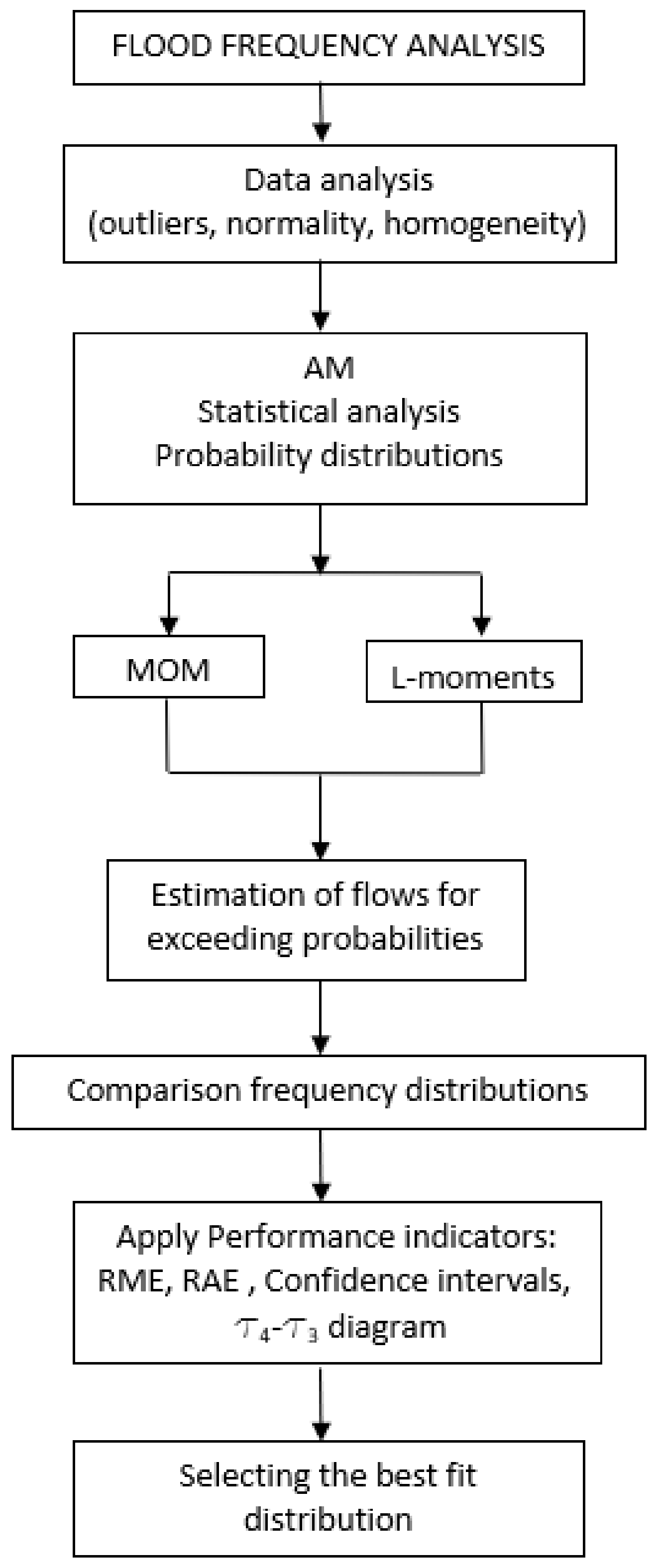
2. Methods
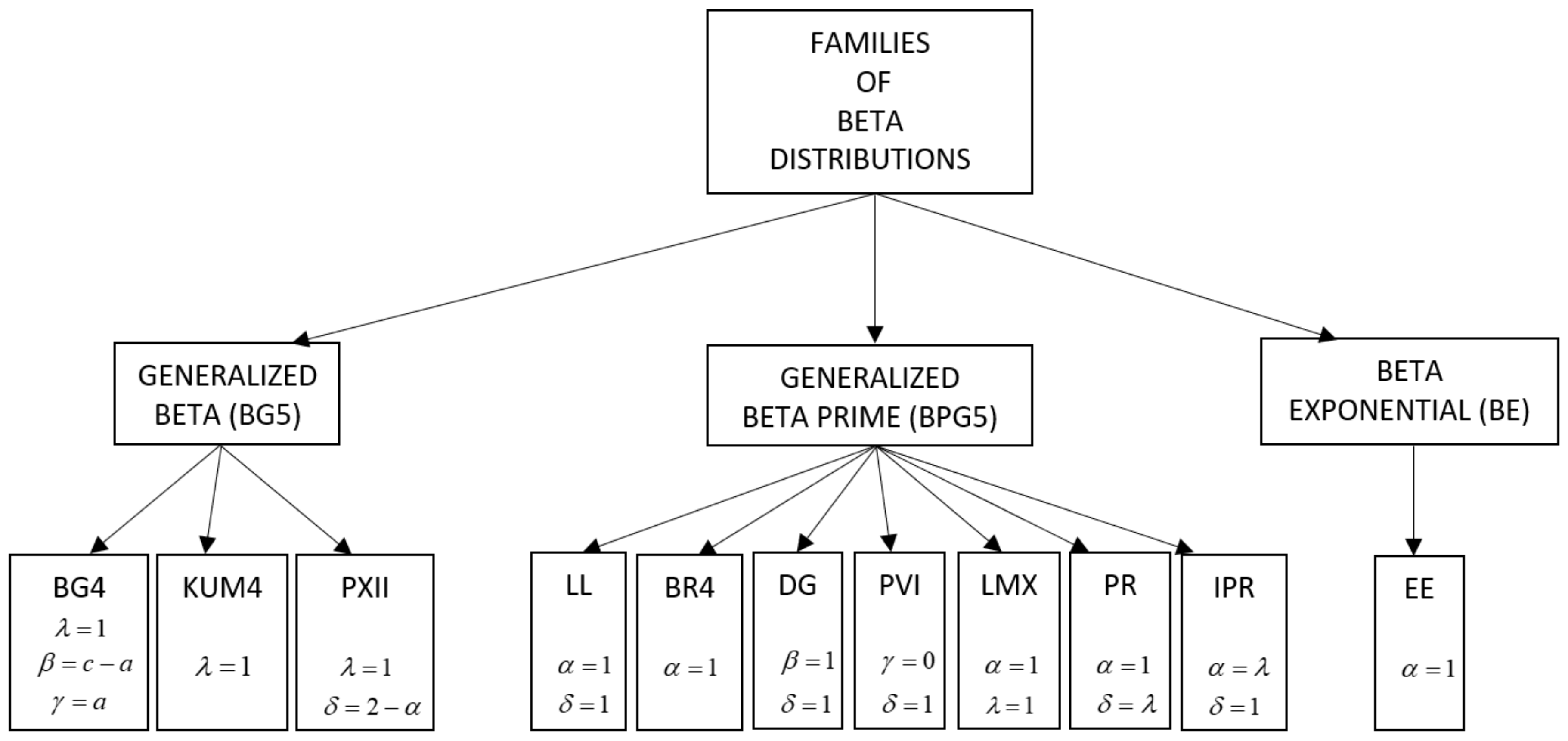
2.1. Probability Distributions
2.2. Parameter Estimation
2.2.1. Beta Generalized by Five Parameters (BG5)
2.2.2. Beta Generalized by Four Parameters (BG4)
2.2.3. Kumaraswamy (KUM4)
2.2.4. Pearson XII (PXII)
2.2.5. Beta Prime Generalized by Five Parameters (BPG5)
2.2.6. Pearson VI (PVI)
2.2.7. Lomax (LMX)
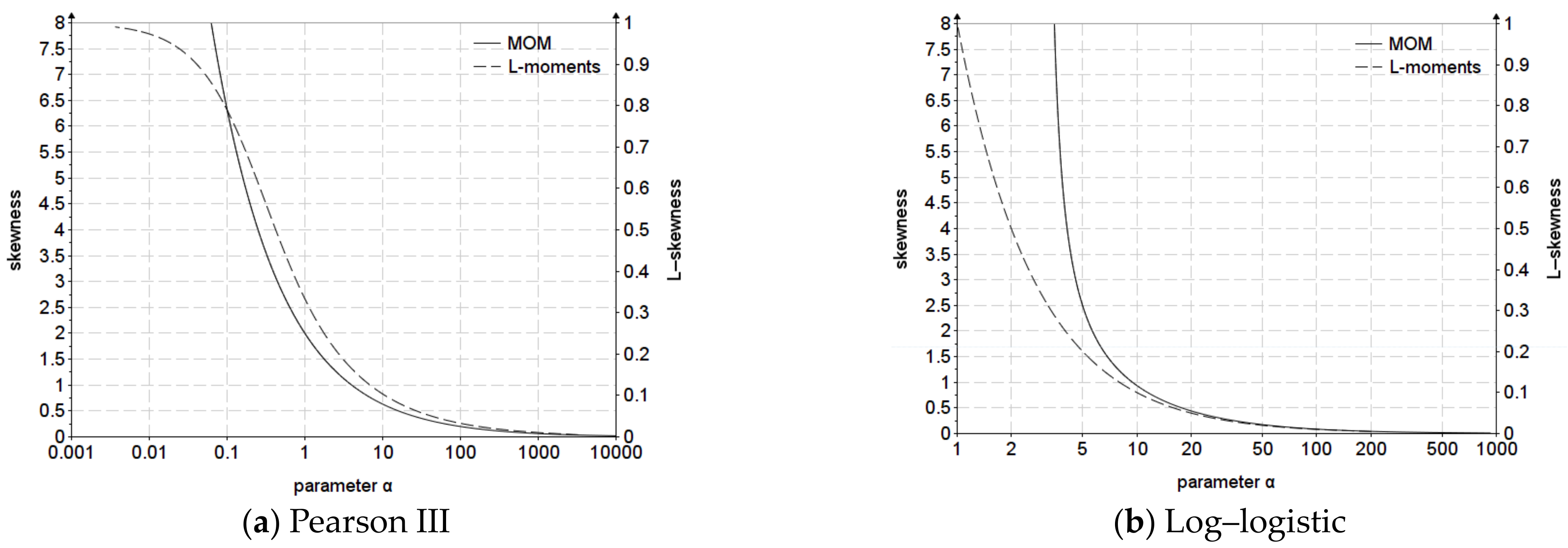
2.2.8. Log–Logistic (LL)
2.2.9. Dagum (DG)
2.2.10. Burr of Four Parameters (BR4)
2.2.11. Paralogistic (PR)
2.2.12. Inverse Paralogistic (IPR)
2.2.13. Generalized Beta Exponential (BEG)
2.2.14. Exponential Exponentiated (EE)
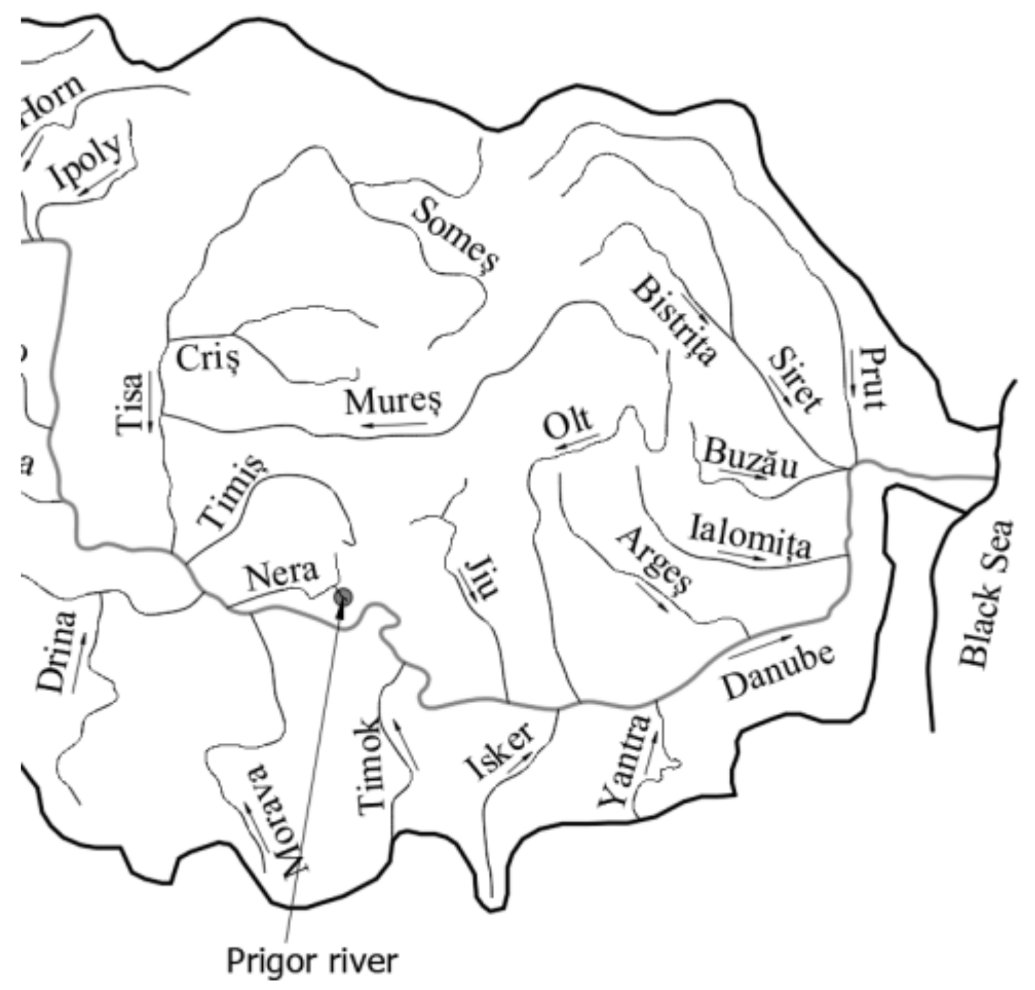
3. Case Study
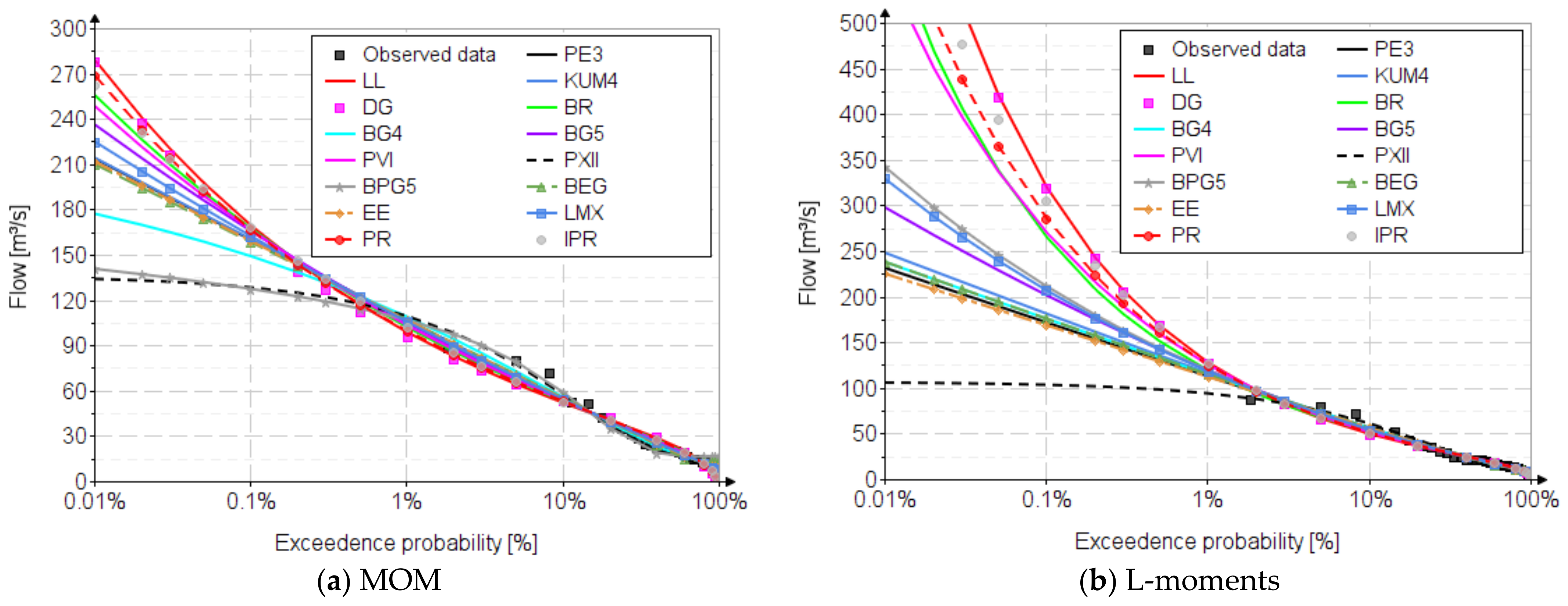
4. Results
5. Discussions
6. Conclusions
Supplementary Materials
Author Contributions
Funding
Institutional Review Board Statement
Informed Consent Statement
Data Availability Statement
Conflicts of Interest
Abbreviations
| MOM | the method of ordinary moments |
| L-moments | the method of linear moments |
| expected value; arithmetic mean | |
| standard deviation | |
| coefficient of variation | |
| coefficient of skewness; skewness | |
| coefficient of kurtosis; kurtosis | |
| linear moments | |
| coefficient of variation based on the L-moments method | |
| coefficient of skewness based on the L-moments method | |
| coefficient of kurtosis based on the L-moments method | |
| central moments (with MOM) | |
| represents the function that generates characteristic moments | |
| Distr. | Distributions |
| RME | relative mean error |
| RAE | relative absolute error |
| xi | observed values |
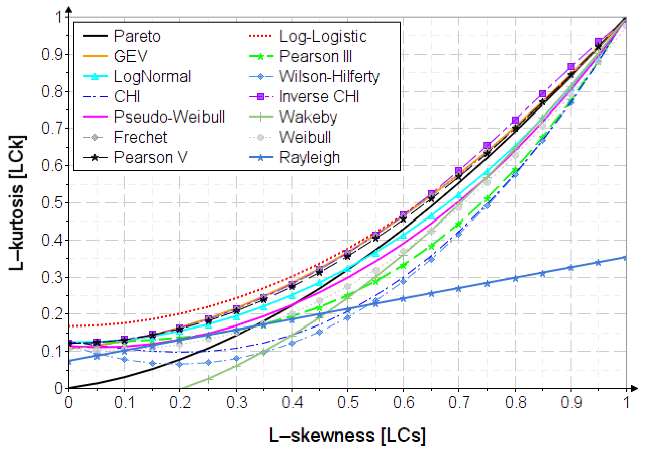
Appendix A. The Variation of L-kurtosis–L-skewness

Appendix B. The Annual Maximum Observed Data from the Prigor River

| Annual Maximum Flows | ||||||||||||
|---|---|---|---|---|---|---|---|---|---|---|---|---|
| 1990 | 1991 | 1992 | 1993 | 1994 | 1995 | 1996 | 1997 | 1998 | 1999 | 2000 | ||
| Flow | [m3/s] | 9.96 | 15 | 10.1 | 14.8 | 7.30 | 21.2 | 18.2 | 21.4 | 13.1 | 14.5 | 35 |
| 2001 | 2002 | 2003 | 2004 | 2005 | 2006 | 2007 | 2008 | 2009 | 2010 | 2011 | ||
| Flow | [m3/s] | 19.9 | 22.1 | 11.8 | 80.3 | 88 | 51.6 | 72.2 | 16.2 | 42.6 | 28.5 | 12.8 |
| 2012 | 2013 | 2014 | 2015 | 2016 | 2017 | 2018 | 2019 | 2020 | ||||
| Flow | [m3/s] | 31.2 | 24.1 | 52.2 | 21.1 | 18.9 | 6.40 | 24.9 | 15.1 | 36.6 | ||
Appendix C. The Relationships for Estimating Skewness and Kurtosis
Appendix D. Built-In Function in Mathcad and Excel
- —returns the value of the Euler gamma function of x;
- —returns the value of the incomplete gamma function of x with parameter a;
- —incomplete Beta, returns the value of the incomplete beta function of x and y with parameter a;
- —returns the inverse cumulative probability distribution for probability p, for beta distribution. This can also be found in other dedicated programs (BETA.INV function in Excel).
- —the digamma function; returns the derivative of the natural logarithm of the gamma function Γ(z).
References
- Popovici, A. Dams for Water Accumulations, Vol. II; Technical Publishing House: Bucharest, Romania, 2002. [Google Scholar]
- STAS 4068/1-82; Maximum Water Discharges and Volumes, Determination of Maximum Water Discharges and Volumes of Watercourses. The Romanian Standardization Institute: Bucharest, Romania, 1982.
- Ilinca, C.; Anghel, C.G. Flood-Frequency Analysis for Dams in Romania. Water 2022, 14, 2884. [Google Scholar] [CrossRef]
- Constantinescu, M.; Golstein, M.; Haram, V.; Solomon, S. Hydrology; Technical Publishing House: Bucharest, Romania, 1956. [Google Scholar]
- Diaconu, C.; Serban, P. Syntheses and Hydrological Regionalization; Technical Publishing House: Bucharest, Romania, 1994. [Google Scholar]
- Bulletin 17B Guidelines for Determining Flood Flow Frequency; Hydrology Subcommittee, Interagency Advisory Committee on Water Data, U.S. Department of the Interior, U.S. Geological Survey, Office of Water Data Coordination: Reston, VA, USA, 1981.
- Bulletin 17C Guidelines for Determining Flood Flow Frequency; U.S. Department of the Interior, U.S. Geological Survey: Reston, VA, USA, 2017.
- Hosking, J.R.M. L-moments: Analysis and Estimation of Distributions using Linear, Combinations of Order Statistics. J. R. Statist. Soc. 1990, 52, 105–124. [Google Scholar] [CrossRef]
- Hosking, J.R.M.; Wallis, J.R. Regional Frequency Analysis, An Approach Based on L-Moments; Cambridge University Press: Cambridge, UK, 1997; ISBN 13 978-0-521-43045-6. [Google Scholar]
- World Meteorological Organization. (WMO-No.100) 2018 Guide to Climatological Practices; WMO: Geneva, Switzerland, 2018. [Google Scholar]
- Rao, A.R.; Hamed, K.H. Flood Frequency Analysis; CRC Press LLC: Boca Raton, FL, USA, 2000. [Google Scholar]
- Guo, C.; Ye, C.; Ding, Y.; Wang, P. A Multi-State Model for Transmission System Resilience Enhancement Against Short-Circuit Faults Caused by Extreme Weather Events. IEEE Trans. Power Deliv. 2021, 36, 2374–2385. [Google Scholar] [CrossRef]
- Ahmad, M.I.; Sinclair, C.D.; Werritty, A. Log-logistic flood frequency analysis. J. Hydrol. 1988, 98, 205–224. [Google Scholar] [CrossRef]
- Domma, F.; Condino, F. Use of the Beta-Dagum and Beta-Singh-Maddala distributions for modeling hydrologic data. Stoch. Environ. Res. Risk Assess. 2017, 31, 799–813. [Google Scholar] [CrossRef]
- Shao, Q.; Wong, H.; Xia, J.; Ip, W.-C. Models for extremes using the extended three-parameter Burr XII system with application to flood frequency analysis/Modèles d’extrêmes utilisant le système Burr XII étendu à trois paramètres et application à l’analyse fréquentielle des crues. Hydrol. Sci. J. 2004, 49, 702. [Google Scholar] [CrossRef]
- Helu, A. The principle of maximum entropy and the probability-weighted moments for estimating the parameters of the Kumaraswamy distribution. PLoS ONE 2022, 17, e0268602. [Google Scholar] [CrossRef]
- Singh, V.P. Entropy-Based Parameter Estimation in Hydrology; Springer Science + Business Media: Dordrecht, The Netherlands, 1998; ISBN 978-90-481-5089-2. ISBN 978-94-017-1431-0 (eBook). [Google Scholar] [CrossRef]
- Nipada, P.; Park, J.-S.; Busababodhin, P. Penalized likelihood approach for the four-parameter kappa distribution. J. Appl. Stat. 2022, 49, 1559–1573. [Google Scholar] [CrossRef]
- Shin, Y.; Park, J.-S. Modeling climate extremes using the four-parameter kappa distribution for r-largest order statistics. Weather. Clim. Extrem. 2023, 39, 100533. [Google Scholar] [CrossRef]
- Masdari, M.; Tahani, M.; Naderi, M.H.; Babayan, N. Optimization of airfoil Based Savonius wind turbine using coupled discrete vortex method and salp swarm algorithm. J. Clean. Prod. 2019, 222, 47–56. [Google Scholar] [CrossRef]
- Anghel, C.G.; Ilinca, C. Hydrological Drought Frequency Analysis in Water Management Using Univariate Distributions. Appl. Sci. 2023, 13, 3055. [Google Scholar] [CrossRef]
- Singh, V.P.; Singh, K. Parameter Estimation for Log-Pearson Type III Distribution by Pome. Hydraul. Eng. 1988, 114, 112–122. [Google Scholar] [CrossRef]
- Srivastava, H.M.; Iqbal, J.; Arif, M.; Khan, A.; Gasimov, Y.S.; Chinram, R. A New Application of Gauss Quadrature Method for Solving Systems of Nonlinear Equations. Symmetry 2021, 13, 432. [Google Scholar] [CrossRef]
- Zajačko, I.; Gál, T.; Sagova, Z.; Mateichyk, V.; Więcek, D. Application of artificial intelligence principles in mechanical engineering. MATEC Web Conf. 2018, 244, 01027. [Google Scholar] [CrossRef]
- Garmendía-Martínez, A.; Muñoz-Pérez, F.M.; Furlan, W.D.; Giménez, F.; Castro-Palacio, J.C.; Monsoriu, J.A.; Ferrando, V. Comparative Study of Numerical Methods for Solving the Fresnel Integral in Aperiodic Diffractive Lenses. Mathematics 2023, 11, 946. [Google Scholar] [CrossRef]
- Crooks, G.E. Field Guide to Continuous Probability Distributions; Berkeley Institute for Theoretical Science: Berkeley, CA, USA, 2019. [Google Scholar]
- Anghel, C.G.; Ilinca, C. Parameter Estimation for Some Probability Distributions Used in Hydrology. Appl. Sci. 2022, 12, 12588. [Google Scholar] [CrossRef]
- López-Rodríguez, F.; García-Sanz-Calcedo, J.; Moral-García, F.J.; García-Conde, A.J. Statistical Study of Rainfall Control: The Dagum Distribution and Applicability to the Southwest of Spain. Water 2019, 11, 453. [Google Scholar] [CrossRef] [Green Version]
- The Romanian Water Classification Atlas, Part I—Morpho-Hydrographic Data on the Surface Hydrographic Network; Ministry of the Environment: Bucharest, Romania, 1992.
- Van Nguyen, T.V.; In-Na, N. Plotting formula for Pearson Type III distribution considering historical information. Environ. Monit. Assess. 1992, 23, 137–152. [Google Scholar] [CrossRef]
- Goel, N.K.; De, M. Development of unbiased plotting position formula for General Extreme Value distributions. Stoch. Hydrol. Hydraul. 1993, 7, 1–13. [Google Scholar] [CrossRef]
- Shaikh, M.P.; Yadav, S.M.; Manekar, V.L. Assessment of the empirical methods for the development of the synthetic unit hydrograph: A case study of a semi-arid river basin. Water Pract. Technol. 2022, 17, 139–156. [Google Scholar] [CrossRef]
- Gu, J.; Liu, S.; Zhou, Z.; Chalov, S.R.; Zhuang, Q. A Stacking Ensemble Learning Model for Monthly Rainfall Prediction in the Taihu Basin, China. Water 2022, 14, 492. [Google Scholar] [CrossRef]
- The Regulations Regarding the Establishment of Maximum Flows and Volumes for the Calculation of Hydrotechnical Retention Constructions; Indicative NP 129-2011; Ministry of Regional Development and Tourism: Bucharest, Romania, 2012.
- Ilinca, C.; Anghel, C.G. Flood Frequency Analysis Using the Gamma Family Probability Distributions. Water 2023, 15, 1389. [Google Scholar] [CrossRef]
- Ibrahim, M.N. Assessment of the Uncertainty Associated with Statistical Modeling of Precipitation Extremes for Hydrologic Engineering Applications in Amman, Jordan. Sustainability 2022, 14, 17052. [Google Scholar] [CrossRef]
- Shao, Y.; Zhao, J.; Xu, J.; Fu, A.; Wu, J. Revision of Frequency Estimates of Extreme Precipitation Based on the Annual Maximum Series in the Jiangsu Province in China. Water 2021, 13, 1832. [Google Scholar] [CrossRef]


| New Elements | Distribution |
|---|---|
| Inverse function | BG5, BG4, PXII, BPG5, PVI, LMX, PR, IPR, BE, EE |
| Complementary cumulative distribution function | PXII, PVI, PMX, PR, IPR, EE |
| The characteristic function which generates moments | BG5, BPG5, BR4, |
| Approximate estimate of the parameters | PXII, LMX, LL, PR, IPR, EE |
| The exact estimate of the parameters | PXII, PVI, LMX, PR, IPR |
| Distr. | |||
|---|---|---|---|
| BG5 | |||
| BG4 | |||
| Kum4 | |||
| PXII | |||
| BPG5 | |||
| PVI | |||
| LMX | |||
| LL | |||
| DG | |||
| BR4 | |||
| PR | |||
| IPR | |||
| BE | |||
| EE |
| Length [km] | Average Stream Slope [‰] | Sinuosity Coefficient [-] | Average Altitude, [m] | Watershed Area, [km2] |
|---|---|---|---|---|
| 33 | 22 | 1.83 | 713 | 153 |
| Prigor | Statistical Indicators | |||||||||||
|---|---|---|---|---|---|---|---|---|---|---|---|---|
| [m3/s] | [m3/s] | [-] | [-] | [-] | [m3/s] | [m3/s] | [m3/s] | [m3/s] | [-] | [-] | [-] | |
| 27.6 | 21.1 | 0.762 | 1.66 | 5.17 | 27.6 | 10.7 | 4.26 | 2.43 | 0.386 | 0.399 | 0.228 | |
| Method of Ordinary Moments (MOM) | ||||||||||||
|---|---|---|---|---|---|---|---|---|---|---|---|---|
| Exceedance Probability [%] | ||||||||||||
| Distr. | 0.01 | 0.1 | 0.5 | 1 | 2 | 3 | 5 | 10 | 20 | 40 | 50 | 80 |
| PE3 | 214 | 160 | 122 | 106 | 90.7 | 81.5 | 69.9 | 54.5 | 39.4 | 24.9 | 20.5 | 12 |
| BG5 | 236 | 166 | 122 | 105 | 88.4 | 79.2 | 68 | 53.5 | 39.7 | 26.3 | 21.9 | 11.9 |
| BG4 | 177 | 149 | 122 | 109 | 94.1 | 84.9 | 72.7 | 55.6 | 38.4 | 22.9 | 18.8 | 13.3 |
| KUM4 | 214 | 160 | 123 | 107 | 90.6 | 81.4 | 69.8 | 54.4 | 39.4 | 25 | 20.6 | 12 |
| PXII | 134 | 128 | 118 | 109 | 98.1 | 89.8 | 77.4 | 57.3 | 36.1 | 20 | 17.2 | 15.4 |
| BPG5 | 141 | 127 | 114 | 107 | 97.3 | 90.2 | 79.1 | 58.9 | 35.1 | 18.8 | 17 | 16.2 |
| PVI | 248 | 166 | 121 | 103 | 87.1 | 78.1 | 67.3 | 53.4 | 40 | 26.8 | 22.3 | 11.7 |
| LMX | 225 | 162 | 122 | 106 | 89.6 | 80.4 | 69.1 | 54.2 | 39.6 | 25.5 | 21.1 | 11.8 |
| LL | 279 | 169 | 117 | 98.7 | 82.7 | 74.2 | 64.3 | 51.9 | 40.4 | 28.6 | 24.3 | 12 |
| DG | 278 | 163 | 113 | 95.6 | 81 | 73.3 | 64.3 | 53 | 41.9 | 29.2 | 24.1 | 10 |
| BR4 | 256 | 167 | 120 | 102 | 85.8 | 77 | 66.4 | 52.9 | 40.1 | 27.4 | 23 | 11.8 |
| PR | 269 | 167 | 117 | 99.6 | 84 | 75.6 | 65.6 | 52.9 | 40.7 | 28 | 23.5 | 11.4 |
| IPR | 262 | 169 | 120 | 102 | 85.4 | 76.5 | 66 | 52.7 | 40.1 | 27.5 | 23.2 | 11.9 |
| BEG | 210 | 158 | 122 | 107 | 91.2 | 82.1 | 70.7 | 55.1 | 39.6 | 24 | 19.1 | 12.7 |
| EE | 212 | 159 | 122 | 107 | 90.9 | 81.7 | 70.2 | 54.6 | 39.4 | 24.7 | 20.3 | 12.1 |
| Method of Linear Moments (L-Moments) | ||||||||||||
|---|---|---|---|---|---|---|---|---|---|---|---|---|
| Exceedance Probability [%] | ||||||||||||
| Distr. | 0.01 | 0.1 | 0.5 | 1 | 2 | 3 | 5 | 10 | 20 | 40 | 50 | 80 |
| PE3 | 231 | 172 | 130 | 113 | 95.4 | 85.3 | 72.7 | 55.9 | 39.7 | 24.4 | 19.8 | 11.4 |
| BG5 | 298 | 202 | 143 | 119 | 97.9 | 86 | 71.9 | 54.2 | 38.4 | 24.4 | 20.2 | 11.8 |
| BG4 | 238 | 176 | 133 | 115 | 96.7 | 86.3 | 73.3 | 56 | 39.4 | 24 | 19.5 | 11.5 |
| KUM4 | 248 | 181 | 136 | 116 | 97.4 | 86.5 | 73.1 | 55.6 | 39.1 | 24 | 19.6 | 11.6 |
| PXII | 106 | 103 | 98.2 | 94 | 87.8 | 82.9 | 75.1 | 61.1 | 43.1 | 23.6 | 18.2 | 11.2 |
| BPG5 | 342 | 211 | 144 | 119 | 97.1 | 85.2 | 71.3 | 54 | 38.4 | 24.4 | 20.2 | 11.8 |
| PVI | 559 | 270 | 159 | 125 | 97.8 | 84 | 68.9 | 51.5 | 37 | 24.6 | 20.8 | 12.3 |
| LMX | 329 | 207 | 142 | 118 | 96.8 | 85.1 | 71.4 | 54.2 | 38.6 | 24.5 | 20.2 | 11.7 |
| LL | 799 | 320 | 169 | 128 | 96.7 | 82.1 | 66.6 | 49.6 | 36.2 | 24.7 | 21.2 | 12.5 |
| DG | 792 | 319 | 168 | 128 | 96.8 | 82.2 | 66.7 | 49.7 | 36.2 | 24.7 | 21.2 | 12.6 |
| BR4 | 600 | 265 | 151 | 119 | 93.7 | 81.3 | 67.7 | 52.1 | 38.4 | 25.1 | 20.6 | 11.3 |
| PR | 647 | 286 | 161 | 125 | 96.7 | 82.9 | 67.9 | 51 | 36.9 | 24.7 | 20.9 | 12.2 |
| IPR | 719 | 305 | 166 | 128 | 97.4 | 82.9 | 67.4 | 50.2 | 36.3 | 24.6 | 21 | 12.6 |
| BEG | 238 | 176 | 133 | 115 | 96.7 | 86.3 | 73.3 | 56 | 39.4 | 24 | 19.5 | 11.5 |
| EE | 225 | 169 | 129 | 112 | 95.1 | 85.2 | 72.8 | 56.2 | 39.8 | 24.3 | 19.7 | 11.4 |
| Distr. | Methods of Parameter Estimation | |||||||||||||
|---|---|---|---|---|---|---|---|---|---|---|---|---|---|---|
| MOM | L-Moments | |||||||||||||
| a | c | a | c | |||||||||||
| PE3 | 0.766 | 24.1 | 9.2 | - | - | - | - | 0.694 | 26.9 | 9.0 | - | - | - | - |
| BG5 | 55.4 | 17,088 | 1.1675 | 0.1375 | 83.9 | - | - | 30.49 | 3558 | 6.51 | 0.1193 | 28.73 | - | - |
| BG4 | 0.404 | 5.59 | - | - | - | 12.7 | 235 | 0.645 | 3937 | - | - | - | 9.43 | 11,125 |
| KUM4 | 0.88 | 59.4 | 8.72 | 1853 | - | - | - | 0.799 | 42.3 | 9.03 | 1853 | - | - | - |
| PXII | 0.203 | 121 | 15.38 | - | - | - | - | 0.354 | 95.9 | 10.7 | - | - | - | - |
| BPG5 | 0.0227 | 141 | 16.2 | 6.3042 | 11.1 | - | - | 0.0632 | 103 | −102 | −104.68 | 560.3 | - | - |
| PVI | 2.7164 | 75.8 | - | 8.446 | - | - | - | 10.31 | 6.29 | - | 3.34 | - | - | - |
| LMX | - | 454.42 | 7.49 | 23.556 | - | - | - | - | 120.9 | 7.95 | 7.137 | - | - | - |
| LL | 5.230 | 52.8 | −28.5 | - | - | - | - | 2.51 | 20.3 | 0.90 | - | - | - | - |
| DG | 4.34 | 46.1 | 0.24 | - | - | - | - | 2.53 | 19.84 | 1.13 | - | - | - | - |
| BR4 | 57.95 | 7.641 | −83.5 | 59.7 | - | - | - | 0.226 | 2.760 | 8.54 | 36.1 | - | - | - |
| PR | 2.2531 | 44.95 | −5.11 | - | - | - | - | 1.6775 | 24.39 | 4.545 | - | - | - | - |
| IPR | 6.9615 | 66.76 | −69.1 | - | - | - | - | 2.7342 | 17.22 | −6.092 | - | - | - | - |
| BEG | 0.0648 | 1.45 | 12.7 | 0.1236 | - | - | - | 28.17 | 790 | 9.43 | 0.645 | - | - | - |
| EE | - | 22.8 | 9.68 | 0.703 | - | - | - | - | 24.5 | 9.164 | 0.662 | - | - | - |
| Distr. | Statistical Measures | |||||||
|---|---|---|---|---|---|---|---|---|
| Methods of Parameter Estimation | Observed Data | |||||||
| MOM | L-Moments | |||||||
| RME | RAE | RME | RAE | |||||
| PE3 | 0.0231 | 0.0841 | 0.0219 | 0.0885 | 0.399 | 0.192 | 0.399 | 0.228 |
| BG5 | 0.0186 | 0.0871 | 0.0165 | 0.0712 | 0.228 | |||
| BG4 | 0.0432 | 0.1198 | 0.0237 | 0.0912 | 0.228 | |||
| KUM4 | 0.0214 | 0.0804 | 0.022 | 0.0843 | 0.228 | |||
| PXII | 0.0660 | 0.2092 | 0.0329 | 0.1338 | 0.118 | |||
| BPG5 | 0.0742 | 0.2481 | 0.0171 | 0.0734 | 0.228 | |||
| PVI | 0.0233 | 0.1098 | 0.0149 | 0.0639 | 0.271 | |||
| LMX | 0.0184 | 0.0784 | 0.0181 | 0.0765 | 0.221 | |||
| LL | 0.0537 | 0.2060 | 0.0165 | 0.0715 | 0.299 | |||
| DG | 0.0480 | 0.2141 | 0.0164 | 0.0714 | 0.300 | |||
| BR4 | 0.0330 | 0.1424 | 0.0214 | 0.0910 | 0.228 | |||
| PR | 0.0398 | 0.1696 | 0.0155 | 0.0672 | 0.272 | |||
| IPR | 0.0357 | 0.1506 | 0.0158 | 0.0678 | 0.295 | |||
| BEG | 0.0441 | 0.1399 | 0.0237 | 0.0912 | 0.228 | |||
| EE | 0.0250 | 0.0872 | 0.0224 | 0.0907 | 0.188 | |||
Disclaimer/Publisher’s Note: The statements, opinions and data contained in all publications are solely those of the individual author(s) and contributor(s) and not of MDPI and/or the editor(s). MDPI and/or the editor(s) disclaim responsibility for any injury to people or property resulting from any ideas, methods, instructions or products referred to in the content. |
© 2023 by the authors. Licensee MDPI, Basel, Switzerland. This article is an open access article distributed under the terms and conditions of the Creative Commons Attribution (CC BY) license (https://creativecommons.org/licenses/by/4.0/).
Share and Cite
Ilinca, C.; Anghel, C.G. Frequency Analysis of Extreme Events Using the Univariate Beta Family Probability Distributions. Appl. Sci. 2023, 13, 4640. https://doi.org/10.3390/app13074640
Ilinca C, Anghel CG. Frequency Analysis of Extreme Events Using the Univariate Beta Family Probability Distributions. Applied Sciences. 2023; 13(7):4640. https://doi.org/10.3390/app13074640
Chicago/Turabian StyleIlinca, Cornel, and Cristian Gabriel Anghel. 2023. "Frequency Analysis of Extreme Events Using the Univariate Beta Family Probability Distributions" Applied Sciences 13, no. 7: 4640. https://doi.org/10.3390/app13074640