Dynamic Analysis and Seat Selection of Bus Driving Comfort under Different Road Conditions

Featured Application

By giving specific road excitation, the differential equations and analytical solutions derived in this paper can be used to quickly estimate the vertical displacement and acceleration of the bus passing through this section of the road. The theoretical results and formulae in this paper can provide some guidelines for bus design and bus driving.

Abstract

The comfort of a bus running on different road conditions is a matter of public concern. In this paper, the differential equations of motion are established for a bus running on different road conditions and the whole driving process is mechanically analyzed. Firstly, the bump degree at different positions is quantitatively analyzed and it is found that the rear row is bumpier on different roads. Then, the relationship between the speed of the bus and the vertical displacement and acceleration is quantitatively described. Regardless of the speed, a similar displacement and acceleration will be eventually achieved, but the speed is higher, and the duration of maximum displacement and acceleration is longer. When the speed is 8 m/s, resonance occurs on the bus during road condition II. Finally, the change in vertical displacement and acceleration under the action of different spring stiffness coefficient ratios of the front and rear wheels is quantitatively analyzed. High stiffness ratios mean less displacement and acceleration. By establishing an actual excitation road surface, the differential equations and analytical solutions in this paper can be used to roughly analyze the mechanical response of a traveling bus. These results can provide some guidance for the design and driving of buses.

1. Introduction

According to the Statistical Bulletin on the Development of the Transportation Industry in 2021 issued by the Chinese government in May 2022, the total mileage of roads in China reached 5.2807 million kilometers, and the number of urban buses and train reached 709,400. Through the study in Malaysia, Kuys et al. [1] found that all countries in the world are facing the problems of increasing urban roads, increasing numbers of buses, and increasing road congestion. With the continuous increase in highway mileage, the comfort of buses has gradually attracted attention. Previous studies found that bus comfort feelings mainly come from noise, temperature, vibration, and acceleration, as listed in Table 1. Among these four factors, vibration and acceleration are the most popular two.

Vertical vibration is the most common form of vibration experienced by passengers in a bus. In 1962, Coermann [2] abstracted the human body into a mechanical impedance structure with multiple degrees of freedom and discussed the biomechanical responses of human body sitting posture to vertical vibration. Gao et al. [3] established a two-degree-of-freedom vertical vibration model of the human body and discussed the influence of body parameters on driver comfort. Bazil et al. [4] discussed the influence of the angle between the fixed backrest and seat on human comfort under different vibration situations through experiments. Their results show that the angle cannot be expressed by a single frequency weighting, rather a multi-frequency weighting function with strong nonlinearity. Xie et al. [5] tested the vibration of a multi-floor three-dimensional passenger station on-site and found that the passenger bus causes floor vertical vibration and thus causes the passenger discomfort in the passenger station. Faster bus speed induces stronger discomfort. The passengers on a train have similar discomfort when the train speed is fast. Zhou et al. [6] verified experimentally that the frequency dependence of the vibration discomfort depends on the acceleration and force at the seat interface with the body, which further verifies that the human body is less affected on the dynamic force than the acceleration. Even a small vertical acceleration can cause discomfort. Vertical acceleration is the main influencing factor in passenger comfort.

Table 1. Research on comfortable attributes influencing bus passengers in previous study.

Comfortable Attributes	Authors, Years, Source	Comfortable Attributes	Authors, Years, Source
Noise	Oborne and Clarke, 1973, [7]	Temperature
	EN 13816, 2002, [8]		EN 13816, 2002, [8]
	Prashanth et al., 2013, [9]		Zhang et al., 2014, [10]
	Zhang et al., 2014, [10]		Almeida et al., 2020, [11]
	Kilikevičius et al., 2020, [12]		Zhou et al., 2022, [13]
	Mathes et al., 2022, [14]
Vibration	Lin et al., 2010, [15]	Accelerations	Wåhlberg, 2006, [16]
	Lin and Chen, 2011, [17]		EN 12299, 2009, [18]
	Sekulić et al., 2013, 2016, 2018, [19,20,21]		Castellanos and Fruett, 2014, [22]
	Castellanos and Fruett, 2014, [22]		Maternini and Cadei, 2014, [23]
	Sekulić and Mladenović, 2016, [24]		Vovsha et al., 2014, [25]
	Zhao et al., 2016, [26]		Eboli et al., 2016, [27]
	Shen et al., 2016, [28]		Barabino et al., 2018, [29]
	Meiping and Wen, 2017, [30]		Nguyen et al., 2019, [31]
	Wang et al., 2020, [32]		Bae et al., 2019, [33]
	Nguyen et al., 2021, [34]		Szumska et al., 2022, [35]

Table 1. Research on comfortable attributes influencing bus passengers in previous study.

Comfortable Attributes	Authors, Years, Source	Comfortable Attributes	Authors, Years, Source
Noise	Oborne and Clarke, 1973, [7]	Temperature
	EN 13816, 2002, [8]		EN 13816, 2002, [8]
	Prashanth et al., 2013, [9]		Zhang et al., 2014, [10]
	Zhang et al., 2014, [10]		Almeida et al., 2020, [11]
	Kilikevičius et al., 2020, [12]		Zhou et al., 2022, [13]
	Mathes et al., 2022, [14]
Vibration	Lin et al., 2010, [15]	Accelerations	Wåhlberg, 2006, [16]
	Lin and Chen, 2011, [17]		EN 12299, 2009, [18]
	Sekulić et al., 2013, 2016, 2018, [19,20,21]		Castellanos and Fruett, 2014, [22]
	Castellanos and Fruett, 2014, [22]		Maternini and Cadei, 2014, [23]
	Sekulić and Mladenović, 2016, [24]		Vovsha et al., 2014, [25]
	Zhao et al., 2016, [26]		Eboli et al., 2016, [27]
	Shen et al., 2016, [28]		Barabino et al., 2018, [29]
	Meiping and Wen, 2017, [30]		Nguyen et al., 2019, [31]
	Wang et al., 2020, [32]		Bae et al., 2019, [33]
	Nguyen et al., 2021, [34]		Szumska et al., 2022, [35]

Uneven ground is the main cause of the vertical vibration of a bus, which seriously affects the comfort of passengers and poses a certain health risk to passengers. In addition to the vertical vibration caused by the bus itself, the uneven ground affects the vertical acceleration. The vibration amplitude is larger, the acceleration is stronger, and the discomfort is stronger. Zhang et al. [36] established the random excitation of the road surface by using the filtered white noise method and analyzed the vertical acceleration caused by the uneven road surface through simulation. They evaluated the ride comfort. Tang et al. [37] used the neural network algorithm to analyze the random excitation of the road surface, thus establishing an annoyance rate model to quantitatively evaluate the comfort of passengers. Bogsjö et al. [38] proposed three new road profile models to quantitatively study passenger comfort and vehicle damage. Chen et al. [39] used experiments to prove the impact of deceleration strips on human comfort. Their results show that the characteristic vibration dose value can be used as a method to evaluate passenger comfort. Agostinacchio et al. [40] proved that an irregular road surface generates a considerable instantaneous dynamic load, which does not contribute to the total response but does affect the human comfort of riding. For the bumpy analysis of the front and rear seats in a bus, Wu and Hao [41] analyzed and demonstrated that the bumpier rear seat is due to the location of the bus gravity and the wheel from the perspective of the differential equation of fixed axle rotation. Song [42] performed a qualitative analysis for the safety requirements of automobiles and reached a similar conclusion. Their common shortcoming is the lack of vehicle dynamics analysis, and their conclusion that the rear row of the bus is bumpier is worthy of further investigation.

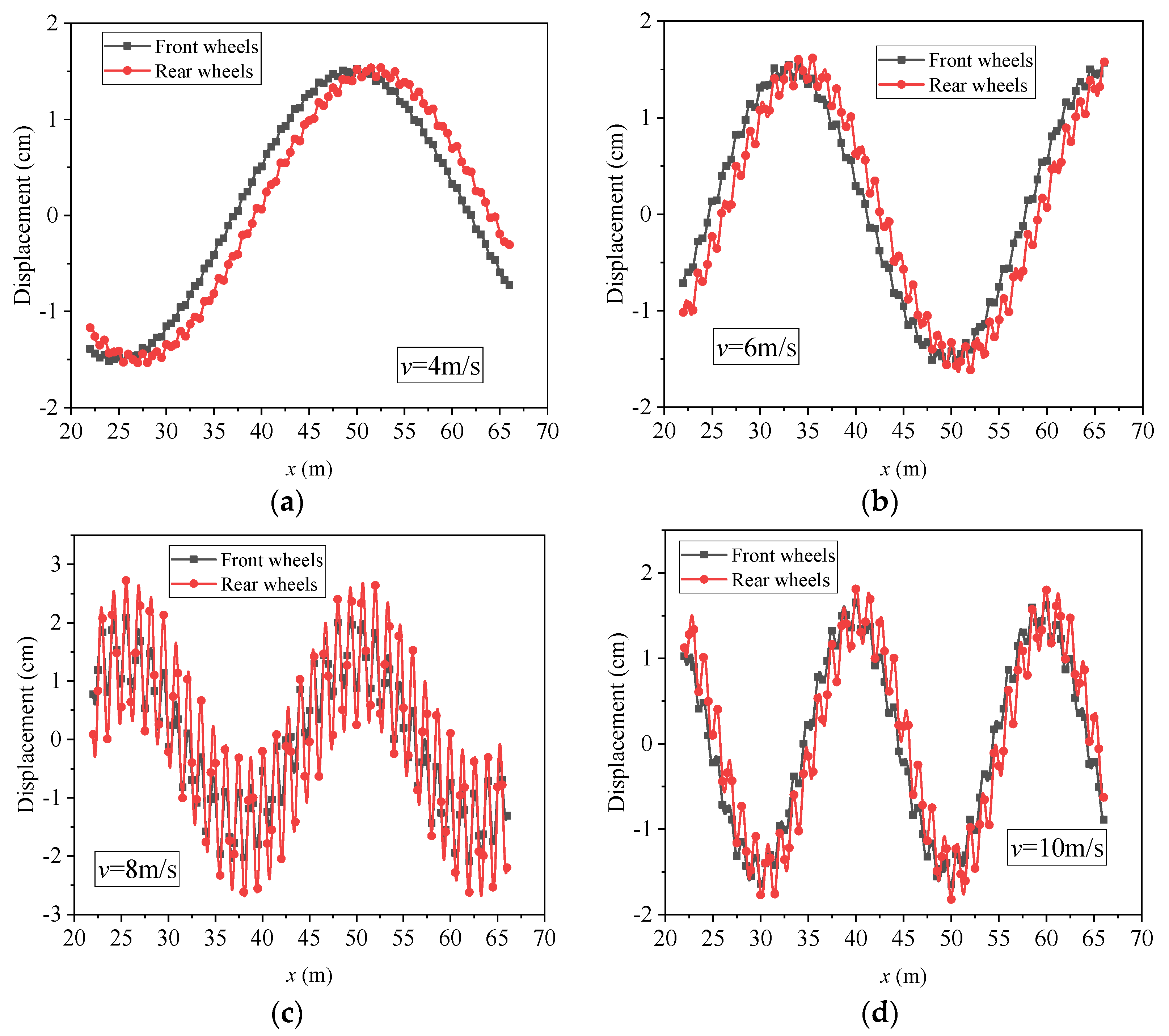
The bus speed is also a major factor affecting the comfort of passengers, especially on uneven roads. Sekulić et al. [19] took the intercity bus IK-301 as an oscillation model with ten degrees of freedom, used the power spectral density of asphalt concrete pavement roughness to generate a total road excitation, and analyzed the impact of vibration on passenger comfort. Bae et al. [33] discussed the impact of speed on passenger comfort, and then proposed a time-optimal speed planning method, which can improve passenger comfort by reasonably planning the driving path. Barabino et al. [43] showed that speed has a great impact on passenger comfort. Nguyen et al. [44] established three relatively simple mathematical models, focusing on the actual driving behavior of urban buses, and studied the impact of acceleration and speed changes on human comfort. In summary, the speed of a bus has a certain impact on the comfort of passengers.

In order to reduce the net displacement of the rear wheel, engineers often assign different values to the spring stiffness of the front wheel and the rear wheel. Zhang et al. [45] used MATLAB to carry out the bus driving matrix and set the front and rear wheel stiffness as 155,400 N/m and 250,000 N/m, respectively, in the calculation. The stability of the bus was analyzed through the derivation of a rigid body dynamics equation. Kong et al. [46] evaluated the quality of the suspension system of the bus through experiments. In the experiment, P-2 parabolic spring was used. The stiffness of the rear wheel was 1.28 times that of the front wheel on average. Long et al. [47] used simulink toolbox to study the influence of vehicle suspension stiffness on bus ride comfort. Their study found that the stiffness of the rear wheel was positively correlated with passenger comfort. Olmeda et al. [48] also explained the influence of the front and rear wheel stiffness coefficient on bus comfort when carrying out a bus lateral dynamics simulation. However, in the equation of its calculation, there are many state variables that have interference and are treated as noise when processing data. It can be seen that the spring stiffness coefficients of the front and rear wheels of the passenger car will also affect the comfort of passengers.

Previous studies focused on vibration and acceleration analysis, but they were too focused on a vehicle analysis of the response of the whole vehicle or the interaction between the vehicle and the uneven ground. Few studies have focused on the coupling analysis of vehicle parts and uneven pavement, and the study of vehicle parts is more conducive to bus design. There are still few studies on the impact of bus speed and the stiffness of front and rear wheel springs on passenger comfort. Therefore, this paper will start with the above problems and conduct quantitative research on the whole process of bus driving based on mathematical and physical methods through self-defining the uneven road surface. This paper is organized as follows: In Section 2, the force of the front and rear wheels of the bus when driving on a flat road is analyzed. In Section 3, the differential equation of the whole process of bus driving is established based on the user-defined uneven road surface and the local displacement characteristics of the front and rear seats of the bus are analyzed. In Section 4, the mechanical responses of the bus under three different road conditions and different driving speeds are analyzed by using the differential equation of motion. In Section 5, the influence of front and rear wheel spring stiffness on passenger car comfort is analyzed. Conclusions are drawn in Section 6.

2. Mechanical Analysis of Bus Running on Horizontal Road

For a bus running on uneven roads, the displacement of the rear seats is significantly greater than that of the front seats. This phenomenon can be clearly observed with the naked eye. Most buses are driven by rear wheels. This means that the engine drives the rear wheels to rotate and move forward depending on the friction between the rear wheels and the ground. In order to make the rear wheel of bus have greater friction with the ground, it is necessary to move the center of gravity of the bus as far back as possible, so as to ensure that the support force of the ground to the rear wheel is greater than that of the front wheel. The center of gravity of the actual running bus is often placed between the front and rear wheels near 1/3 of the rear wheels. This can ensure that the rear wheels bear 2/3 of the vehicle weight and the front wheels bear 1/3 of the vehicle weight.

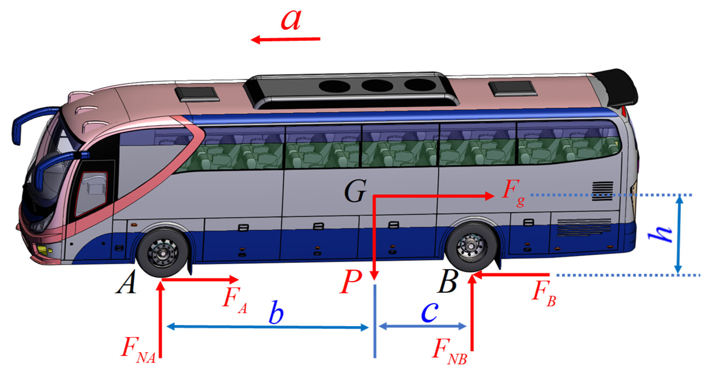
This section analyzes the force of a bus when the bus is normally running on a horizontal road. All bodies of the bus are taken as the rigid bodies to establish the mechanical model bus as shown in Figure 1. The bus is assumed to move in a horizontal straight line with acceleration a (m/s²), where the total mass of the bus is m (kg), the height of the center of mass G from the ground is h (m), and the distance from the front and rear axles to the vertical line of the center of mass is equal to b (m) and c (m), respectively.

Using D’Alembert’s principle [49], the added virtual inertial force is

$$F_g=ma$$

(1)

The bus gravity is

$$P=mg$$

(2)

where F_g is the inertial force, N; P is the gravity, N; g is the acceleration of gravity, m/s².

Moment analysis at point A of the front wheel obtains

$${\displaystyle \sum M_A=0}: bP+h{F}_g-\left(b+c\right)F_{NB}=0$$

(3)

Similarly, the moment analysis at point B of the front wheel is expressed as

$${\displaystyle \sum M_B=0}: \left(b+c\right)F_{NA}+h{F}_g-cP=0$$

(4)

where F_NA (N) is the ground support force on the front wheels and F_NB (N) is the ground support force on the rear wheels.

According to Equations (1)–(4), one can obtain

$$F_{NA}=m\frac{-ha+cg}{b+c} F_{NB}=m\frac{bg+ha}{b+c}$$

(5)

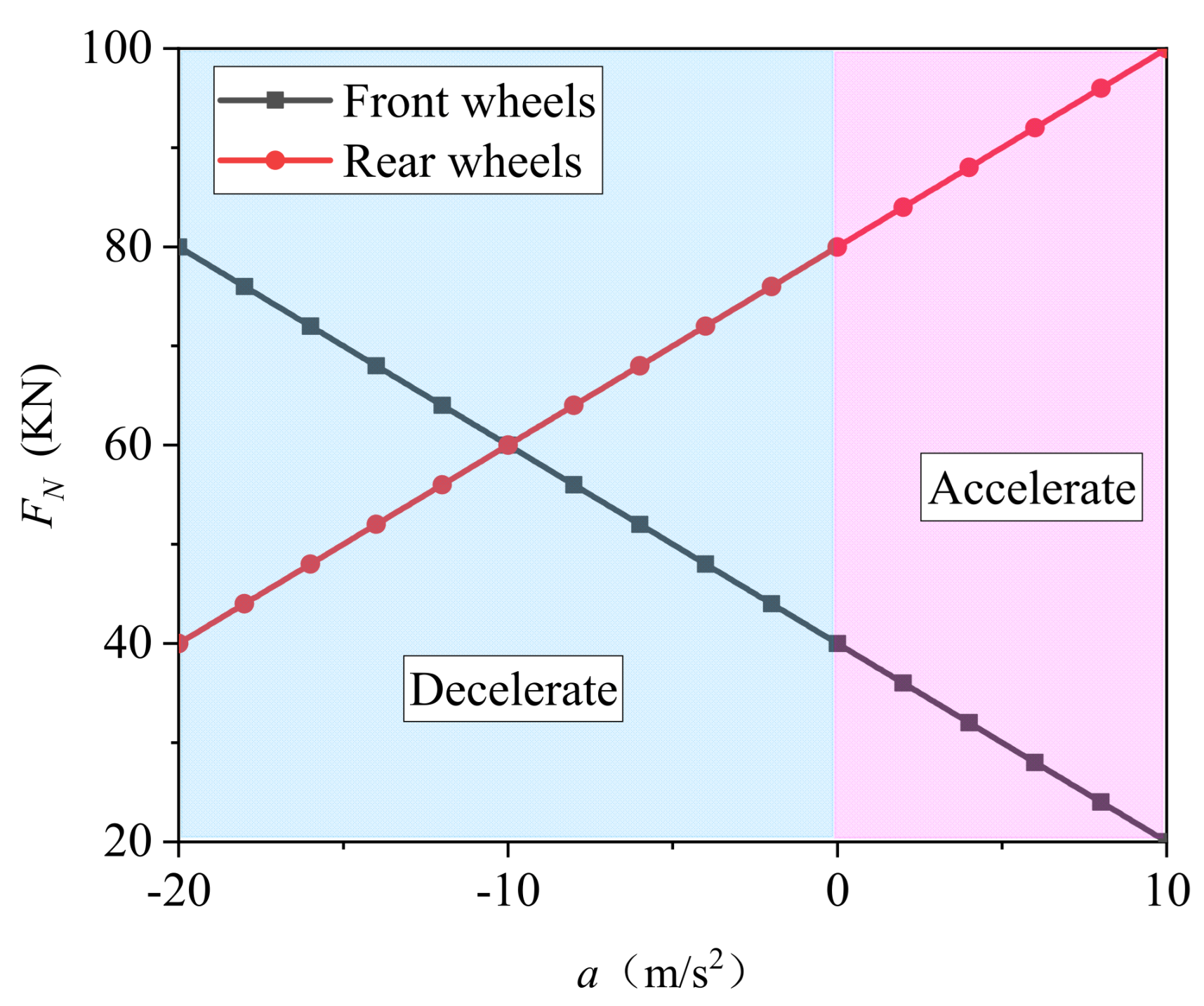
Taking the Yutong ZK6105HNGS1 bus [50] as an example, the whole-body mass of the bus is 12,000 kg, the body length is 10 m, the height of the gravity center is 1.5 m, the wheelbase is 9 m, the front wheel is 1/3 from the center of gravity, and the rear wheel is 2/3 from the center of gravity. The relationship between the support force and the acceleration of the front and rear wheels on the ground is shown in Figure 2, which is based on Equation (5). The normal maximum acceleration of the bus is 8 m/s² [51], and the braking acceleration is −10 m/s² [52]. The critical takeoff means that the support force F_N is zero. Figure 2 shows that the critical takeoff condition is met with difficulty when the bus is running on a horizontal road. When the bus acceleration a > −10 m/s², the supporting force of the ground to the rear wheel is always greater than that of the front wheel. According to the isolation method, it is not difficult to infer that the passengers in the rear row bear greater acceleration and greater acceleration changes.

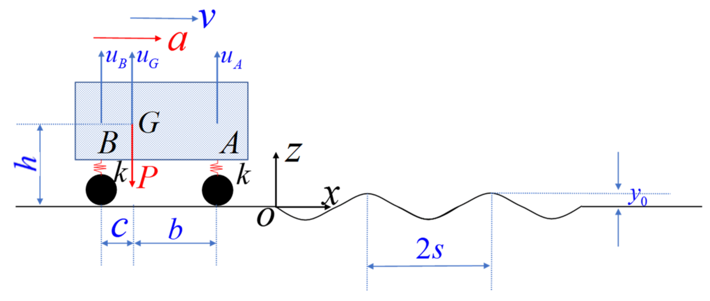
3. Mechanical Analysis of a Bus Running on an Uneven Road

The smoothness of the road surface seriously affects the safety of buses [53]. The fluctuation of ISO-B pavement is 0.1 m [54], and some vertical acceleration reaches 2 m/s², which is more serious in rural regions [55]. Zhang et al. [56] used the power spectral density formula of road roughness in the Chinese national standard GB/T7031-2005 to inverse the road roughness. They obtained the maximum difference of 0.2 m and an acceleration of 2.5 m/s². When the human body feels a vertical acceleration above 0.5 m/s², it begins to feel obvious discomfort [36,57]. In order to facilitate mechanical analysis, the bus is reasonably simplified as a plane problem and the displacement of the bus is analyzed. The road surface is assumed to be y = hcos (2πx/s) and x = vt. The carriage and tire of the bus are connected by the spring coefficient k. It is worth noting that the effect of dampers will be not considered in this paper, which means that energy does not decay with the progress of the bus. All conclusions of the analysis are based on the bus limit state, which is conducive to a better explanation of the problem. The vertical displacement of the front wheel, the center of gravity, and the rear wheel are defined as u_A, u_G, and u_B, respectively. s is the difference between two adjacent wave peaks with a convex periodic boundary. Other parameters are consistent with Figure 1. Three road conditions will be analyzed when the bus passes through the uneven road section. The initial state includes two: First, the spring bears the bus gravity and produces a certain displacement. Second, the front wheel position of the bus has just reached the starting point of the uneven road section. The analytical model is shown in Figure 3. In this section, if there is no special explanation, the displacement is considered as vertical displacement, and the acceleration is also considered as vertical acceleration. Downhill means that the bus is in road condition I (0 ≤ x ≤ (b + c)) and climbing means that the bus is in road condition III (2ns ≤ x ≤ 2ns + (b + c) (n ∈ N*)).

3.1. Road Condition I

The bus moves forward. The front wheel drives into the uneven road section, but the rear wheel is still in the flat road section; thus, the bus travel distance is 0 ≤ x ≤ (b + c). The vertical displacement increment of two points A and B of the bus is denoted as δ_A and δ_B. Since the front wheel has driven into the pit, there is a geometric relationship:

$${\delta }_A=u_A-y_A {\delta }_B=u_B-y_B$$

(6)

where y_A and y_B are the vertical coordinates of the front and rear wheels of the bus.

$$y_A=h\cos \left(\frac{2\pi }{s}x\right) y_B=h$$

(7)

All bodies of the bus are regarded as rigid bodies. The vertical displacement coordinate u_G at the center of gravity can be solved by using a similar triangle method:

$$u_G=\frac{c{u}_A+b{u}_B}{b+c}$$

(8)

The upper part of the bus is analyzed by the free-body method. The force analysis is shown in Figure 4:

The equation of motion is

$$k{\delta }_A+k{\delta }_B=-m\frac{d^2{u}_G}{d{t}^2}$$

(9)

The equilibrium equation for calculating the moment of force at point G is

$$k{\delta }_{A}b-k{\delta }_{B}c=0$$

(10)

Combining Equations (8)–(10) obtains the differential equation of motion:

$$k\left(b+c\right)\left(u_A-y_A\right)=-m\frac{b^2+c^2}{b+c}\frac{d^2{u}_A}{d{t}^2}$$

(11)

Its general solution is obtained with

$$u_A=y_A+C_1\cos \left[\frac{\left(b+c\right)}{\sqrt{b^2+c^2}}\sqrt{\frac{k}{m}}t\right]+C_2\sin \left[\frac{\left(b+c\right)}{\sqrt{b^2+c^2}}\sqrt{\frac{k}{m}}t\right]$$

(12)

where C₁ and C₂ are the coefficients to be determined by boundary conditions.

Combining Equations (6) and (10) obtains u_B:

$$u_B=\frac{b}{c}\left(u_A-y_A\right)+y_B$$

(13)

When x = 0 and the front wheel moves to point O, the boundary condition is

$$u_A=h \frac{d{u}_A}{dt}=0$$

(14)

Therefore, the coefficients in Equation (12) can be determined as

$$C_{11}=h\left[1-\cos \left(\frac{2\pi }{s}x\right)\right] C_{21}=0$$

(15)

The vertical displacement of bus points A and B is then expressed as

$$\left\{\begin{array}{l}{u}_{A1}=h\cos \left(\frac{2\pi }{s}x\right)+h\left[1-\cos \left(\frac{2\pi }{s}x\right)\right]\cos \left[\frac{\left(b+c\right)}{\sqrt{b^2+c^2}}\sqrt{\frac{k}{m}}t\right]\\ u_{B1}=h+\frac{bh}{c}\left[1-\cos \left(\frac{2\pi }{s}x\right)\right]\cos \left[\frac{\left(b+c\right)}{\sqrt{b^2+c^2}}\sqrt{\frac{k}{m}}t\right]\end{array}\right.$$

(16)

The last subscript 1 in Equations (15) and (16) denotes road condition I.

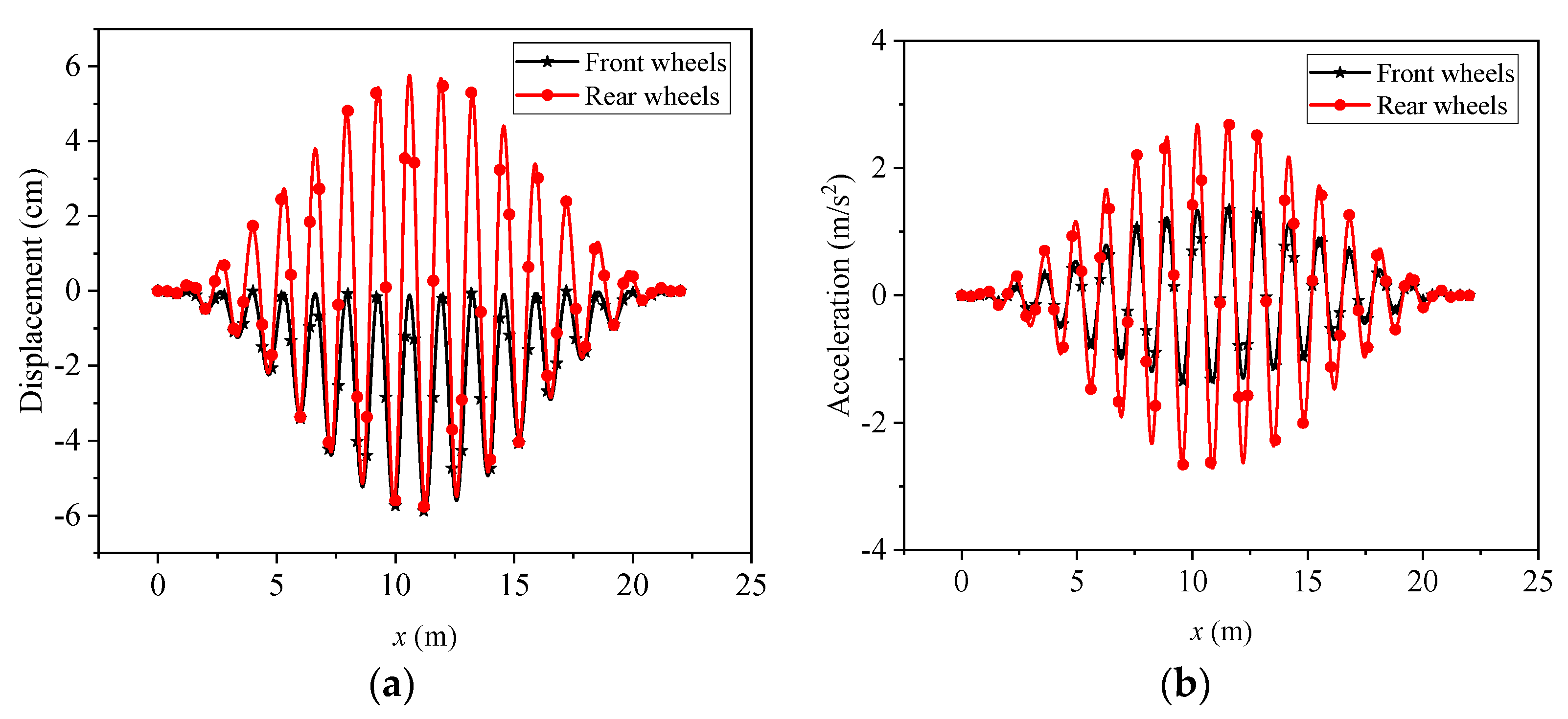
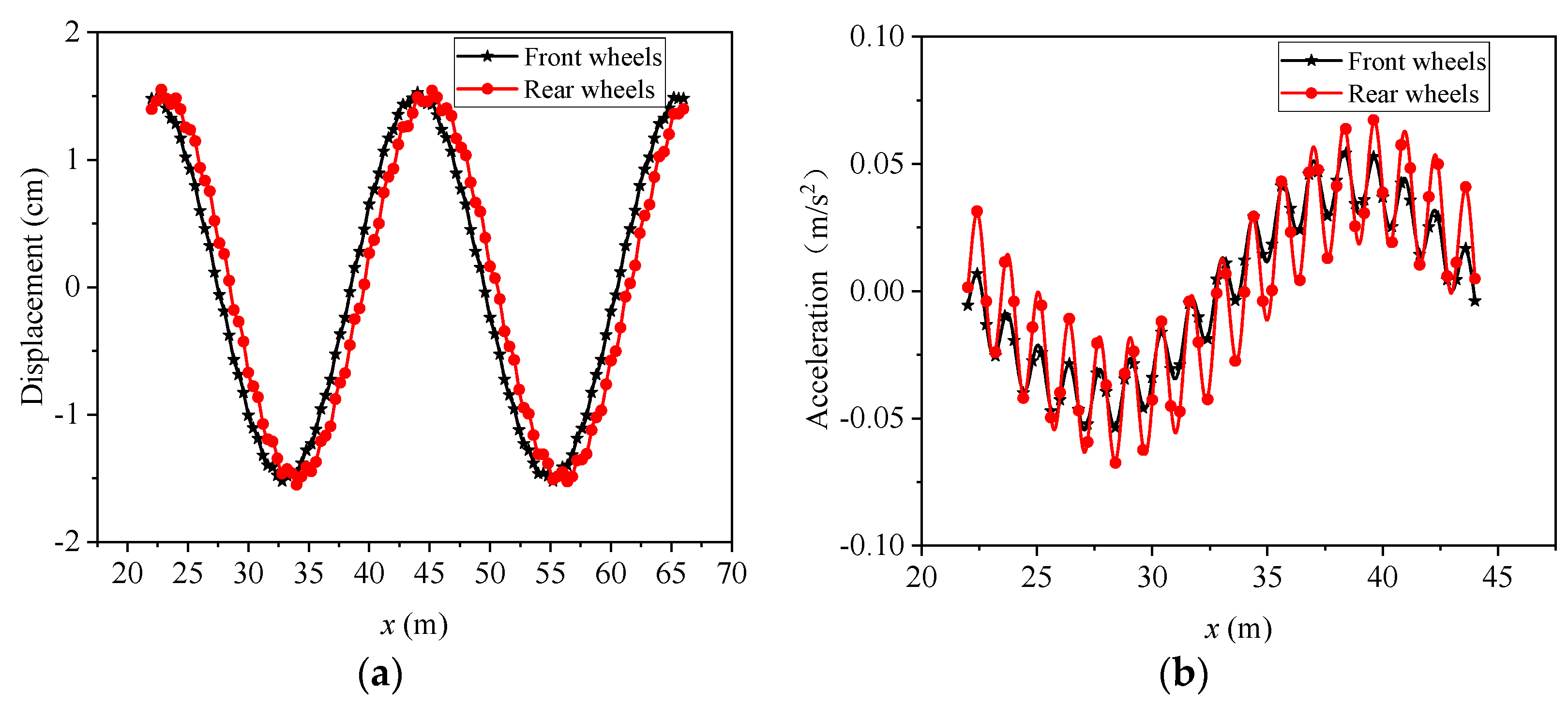
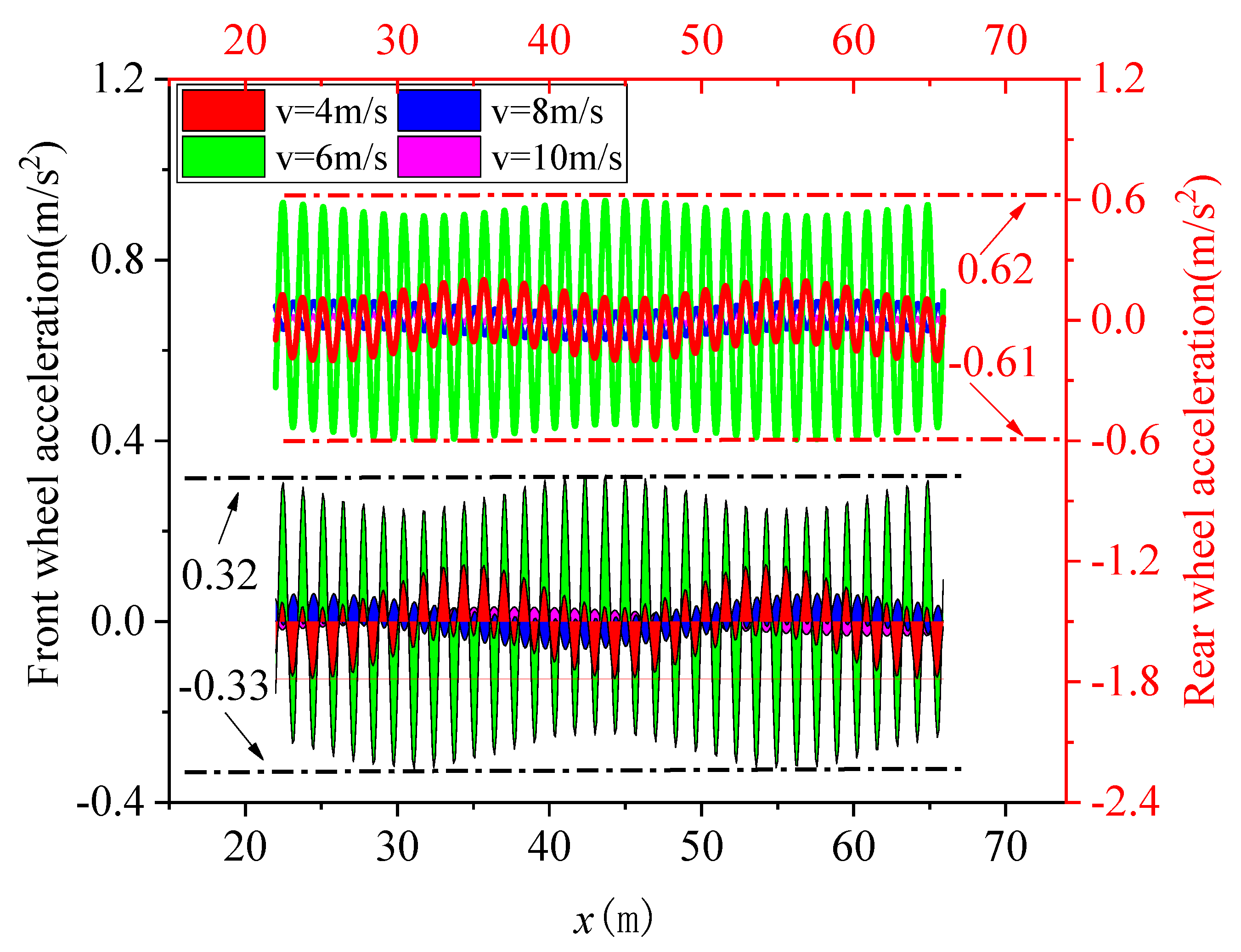
This paper uses MATLAB to solve Equation (16). Figure 5 shows the result of only net displacement, which means the change in displacement and acceleration of the front and rear wheels in the first stage. The maximum net displacement difference is 5.93 cm at the front wheel and 11.86 cm at the rear wheel. When the front wheel drives on the uneven road and the rear wheel is still on the flat road, the displacement near the rear wheel position is greater. The net vertical acceleration of the front and rear wheels is more than 3 m/s², the peak net acceleration of the rear wheels is 5.31 m/s², and the peak acceleration of the front wheels is 3.32 m/s². The rear wheel acceleration is generally higher than the front wheel acceleration. Thus, the rear wheels are bumpier in the road condition I.

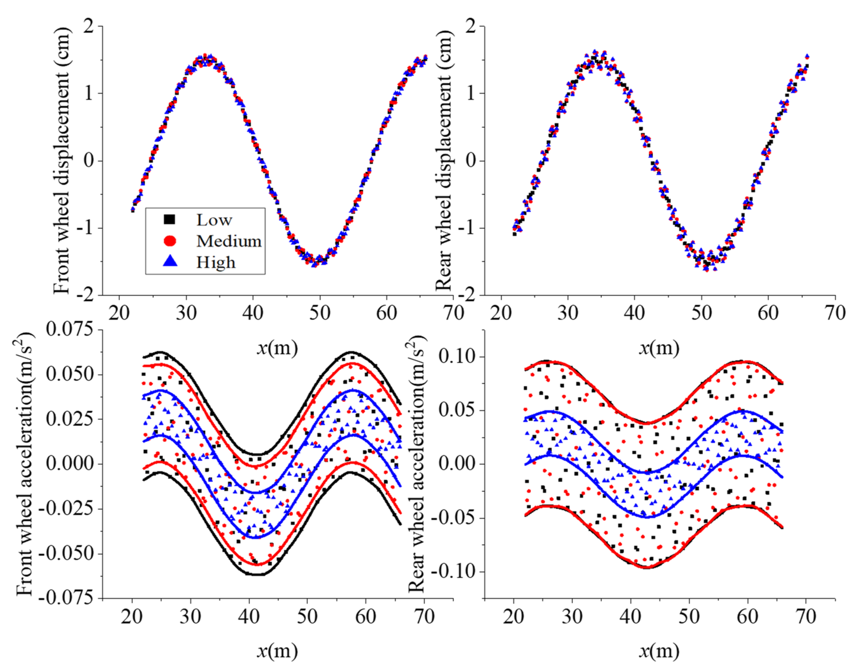
3.2. Road Condition II

Both the front and rear wheels drive into an uneven road section, the bus position is (b + c) ≤ x ≤ 2ns (n ∈ N*). N* is a positive integer. The general differential equation of bus motion is still Equation (11). Its boundary conditions at this stage become the following: when x = b + c, the motion state of road condition II should satisfy Equation (16) in road condition I. The continuity of bus displacement is

$$u_{A1}=u_{A2} u_{B1}=u_{B2}$$

(17)

The subscript 2 represents road condition II.

When x = 2ns (n ∈ N*), the front and rear wheels are all located on uneven road sections. The instantaneous state of the rear wheel entering the uneven road section is

$$u_B=h \frac{d{u}_B}{dt}=0$$

(18)

The status of the front and rear wheels in this process is

$$y_A=h\cos \left(\frac{2\pi }{s}x\right) y_B=h\cos \left[\frac{2\pi }{s}\left(x-b-c\right)\right]$$

(19)

The coefficients obtained by Equations (17)–(19) and Equation (12) are

$$\left\{\begin{array}{l}{C}_{12}=-\frac{c\left(-h+h\cos \left[\frac{2\left(-b-c+2ns\right)\pi }{s}\right]\right)\cos \left[\frac{2\left(b+c\right)\sqrt{k}ns}{\sqrt{b^2+c^2}\sqrt{m}v}\right]}{b\left(\cos {\left[\frac{2\left(b+c\right)\sqrt{k}ns}{\sqrt{b^2+c^2}\sqrt{m}v}\right]}^2+\sin {\left[\frac{2\left(b+c\right)\sqrt{k}ns}{\sqrt{b^2+c^2}\sqrt{m}v}\right]}^2\right)}\\ C_{22}=-\frac{c\left(-h+h\cos \left[\frac{2\left(-b-c+2ns\right)\pi }{s}\right]\right)\csc \left[\frac{2\left(b+c\right)\sqrt{k}ns}{\sqrt{b^2+c^2}\sqrt{m}v}\right]}{b\left(1+\cot {\left[\frac{2\left(b+c\right)\sqrt{k}ns}{\sqrt{b^2+c^2}\sqrt{m}v}\right]}^2\right)}\end{array}\right.$$

(20)

Then, the vertical displacements at bus points A and B are

$$\left\{\begin{array}{l}{u}_{A2}=h\cos \left(\frac{2\pi }{s}x\right)-\frac{c\left(-h+h\cos \left[\frac{2\left(-b-c+2ns\right)\pi }{s}\right]\right)\cos \left[\frac{2\left(b+c\right)\sqrt{k}ns}{\sqrt{b^2+c^2}\sqrt{m}v}\right]}{b\left(\cos {\left[\frac{2\left(b+c\right)\sqrt{k}ns}{\sqrt{b^2+c^2}\sqrt{m}v}\right]}^2+\sin {\left[\frac{2\left(b+c\right)\sqrt{k}ns}{\sqrt{b^2+c^2}\sqrt{m}v}\right]}^2\right)}\cos \left[\frac{\left(b+c\right)}{\sqrt{b^2+c^2}}\sqrt{\frac{k}{m}}t\right]\\ -\frac{c\left(-h+h\cos \left[\frac{2\left(-b-c+2ns\right)\pi }{s}\right]\right)\csc \left[\frac{2\left(b+c\right)\sqrt{k}ns}{\sqrt{b^2+c^2}\sqrt{m}v}\right]}{b\left(1+\cot {\left[\frac{2\left(b+c\right)\sqrt{k}ns}{\sqrt{b^2+c^2}\sqrt{m}v}\right]}^2\right)}\sin \left[\frac{\left(b+c\right)}{\sqrt{b^2+c^2}}\sqrt{\frac{k}{m}}t\right]\\ u_{B2}=h\cos \left[\frac{2\pi }{s}\left(x-b-c\right)\right]-\frac{\left(-h+h\cos \left[\frac{2\left(-b-c+2ns\right)\pi }{s}\right]\right)\cos \left[\frac{2\left(b+c\right)\sqrt{k}ns}{\sqrt{b^2+c^2}\sqrt{m}v}\right]}{\left(\cos {\left[\frac{2\left(b+c\right)\sqrt{k}ns}{\sqrt{b^2+c^2}\sqrt{m}v}\right]}^2+\sin {\left[\frac{2\left(b+c\right)\sqrt{k}ns}{\sqrt{b^2+c^2}\sqrt{m}v}\right]}^2\right)}\cos \left[\frac{\left(b+c\right)}{\sqrt{b^2+c^2}}\sqrt{\frac{k}{m}}t\right]\\ -\frac{\left(-h+h\cos \left[\frac{2\left(-b-c+2ns\right)\pi }{s}\right]\right)\csc \left[\frac{2\left(b+c\right)\sqrt{k}ns}{\sqrt{b^2+c^2}\sqrt{m}v}\right]}{\left(1+\cot {\left[\frac{2\left(b+c\right)\sqrt{k}ns}{\sqrt{b^2+c^2}\sqrt{m}v}\right]}^2\right)}\sin \left[\frac{\left(b+c\right)}{\sqrt{b^2+c^2}}\sqrt{\frac{k}{m}}t\right]\end{array}\right.$$

(21)

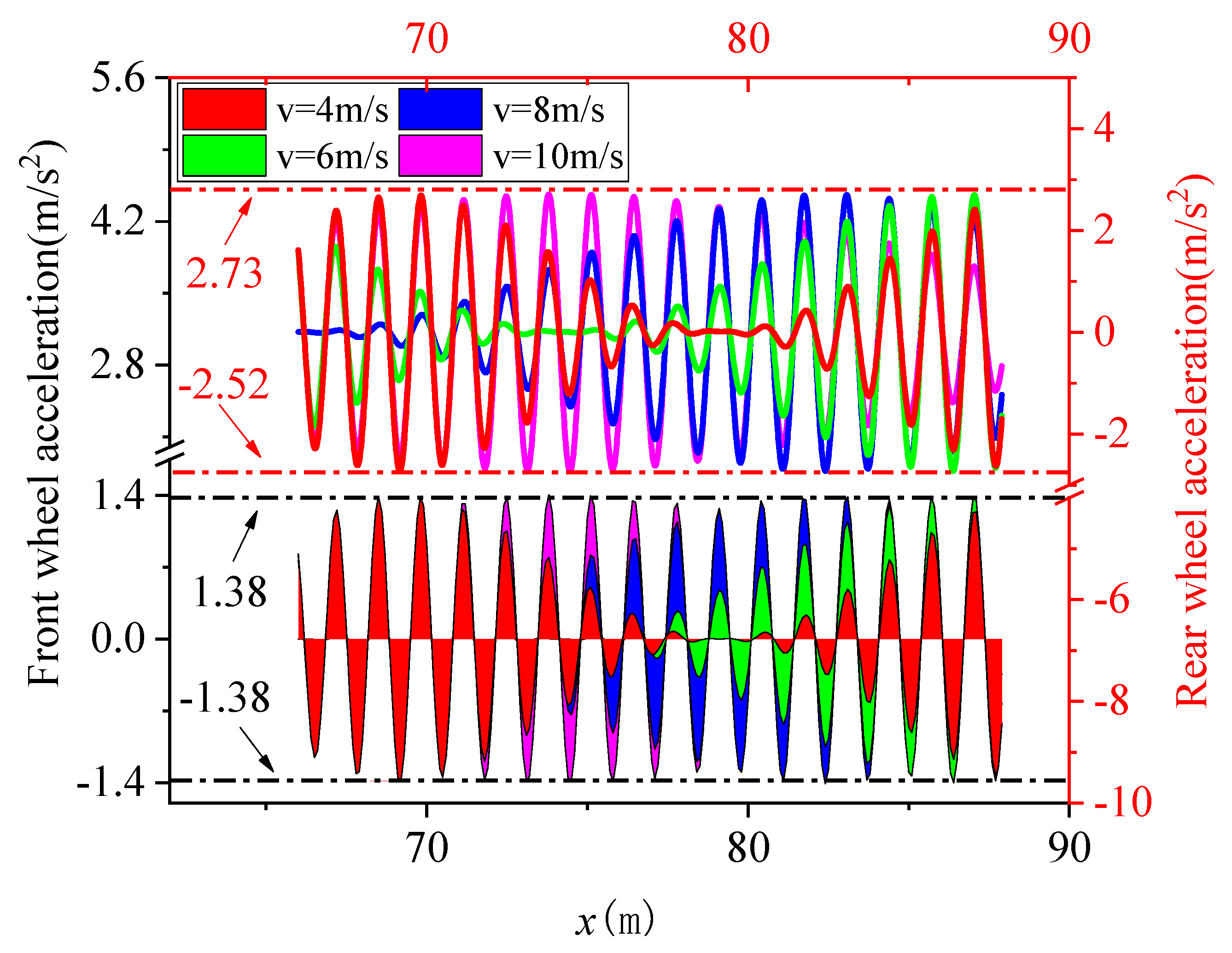
Equation (21) is still solved by MATLAB and Figure 6 is the net displacement. At this time, the maximum net displacement difference is 3.05 cm at the front wheel and 3.1 cm at the rear wheel. Their displacement difference is not obvious in Figure 6a. This may be due to the fact that the uneven road surface is larger than the body span in a single cycle. The vertical positions of the front wheel and the rear wheel are basically in synchronization. The net vertical acceleration of the front and rear wheels is more than 0.1 m/s², the net peak acceleration is 0.14 m/s² at the rear wheels and 0.1 m/s² at the front wheels. The acceleration is still higher at the rear wheels than at the front wheels. This result can still be used as an argument for the rear row being bumpier, although the difference is small or not salient.

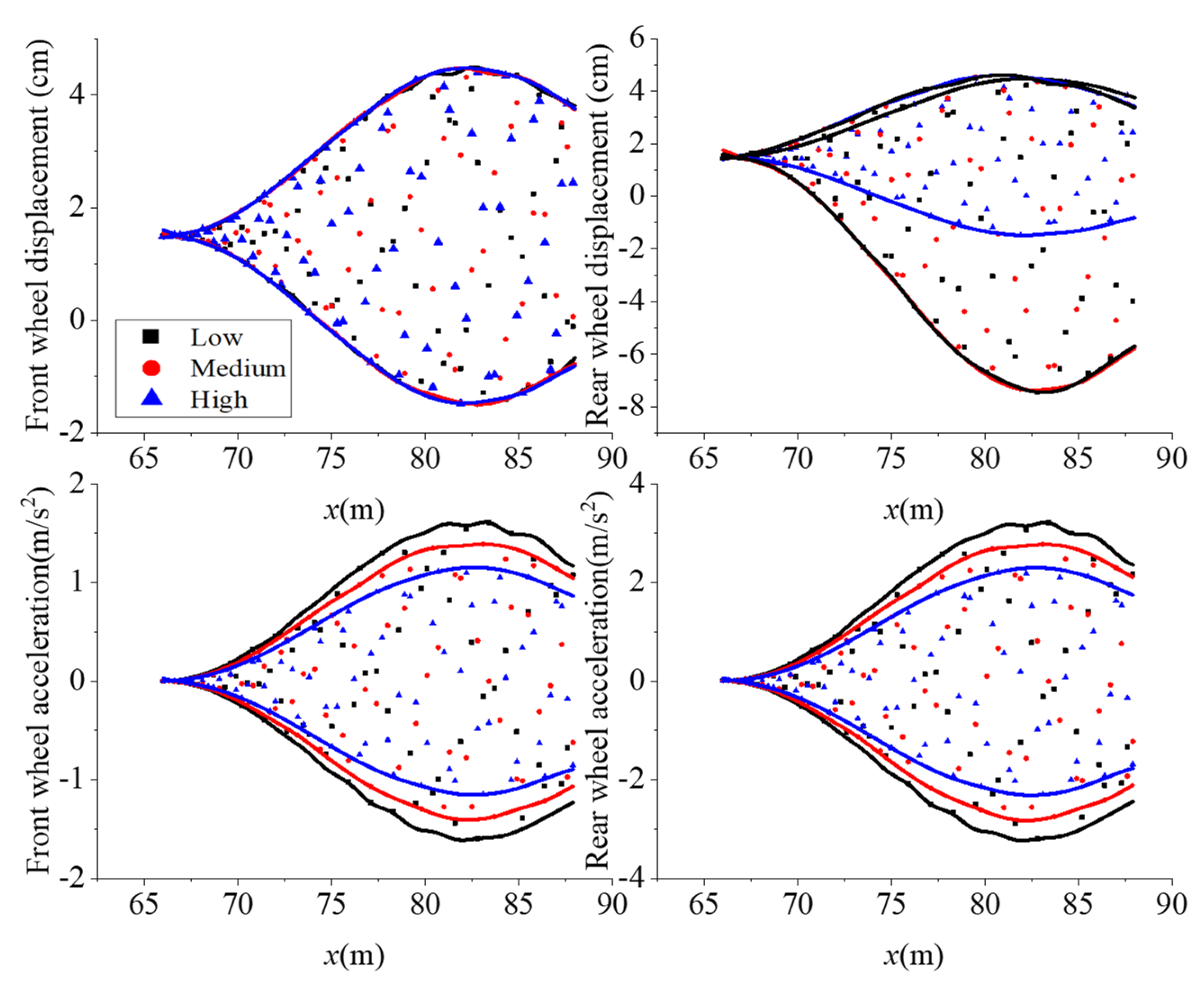
3.3. Road Condition III

The front wheel drives into the flat section, but the rear wheel is still in the uneven section. At this time, the bus position is 2ns ≤ x ≤ 2ns + (b + c) (n ∈ N*). The differential equation of motion in the road condition III is still Equation (11). When x = 2ns (n ∈ N*), the motion state of road condition III should satisfy Equation (21) when x = 2ns (n ∈ N*) in road condition II. The continuity of the bus displacement satisfies

$$u_{A2}=u_{A3} u_{B2}=u_{B3}$$

(22)

The subscript 3 represents road condition III.

When x = 2ns + (b + c) (n ∈ N*), the front wheel has just entered the flat section and the rear wheel is still in the uneven section. The instantaneous state of the front wheel entering the flat road section is

$$u_A=h \frac{d{u}_A}{dt}=0$$

(23)

The statuses of the front and rear wheels in this process are

$$y_A=h y_B=h\cos \left[\frac{2\pi }{s}\left(x-b-c\right)\right]$$

(24)

The coefficients can be determined by Equations (22)–(24) and Equation (12) as

$$C_{13}=h\left[1-\cos \left(\frac{2\pi }{s}x\right)\right] C_{23}=0$$

(25)

The vertical displacements at bus points A and B are

$$\left\{\begin{array}{l}{u}_{A3}=h+h\left[1-\cos \left(\frac{2\pi }{s}x\right)\right]\cos \left[\frac{\left(b+c\right)}{\sqrt{b^2+c^2}}\sqrt{\frac{k}{m}}t\right]\\ u_{B3}=h\cos \left[\frac{2\pi }{s}\left(x-b-c\right)\right]+\frac{bh}{c}\left[1-\cos \left(\frac{2\pi }{s}x\right)\right]\cos \left[\frac{\left(b+c\right)}{\sqrt{b^2+c^2}}\sqrt{\frac{k}{m}}t\right]\end{array}\right.$$

(26)

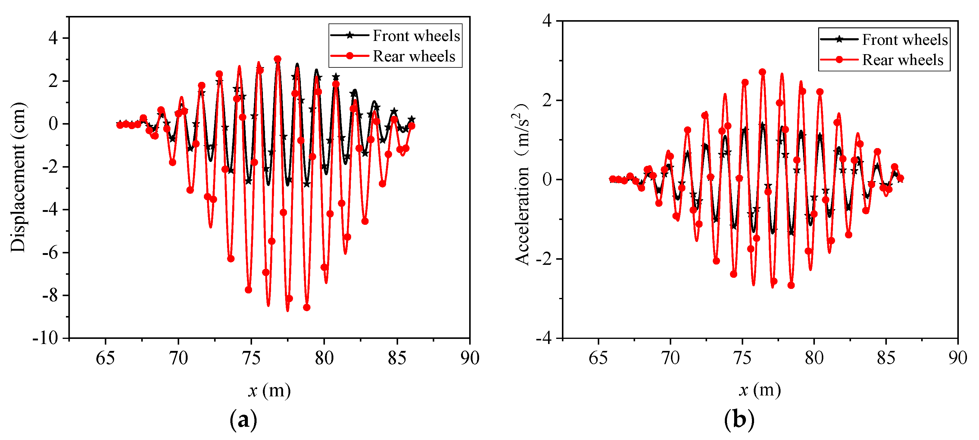
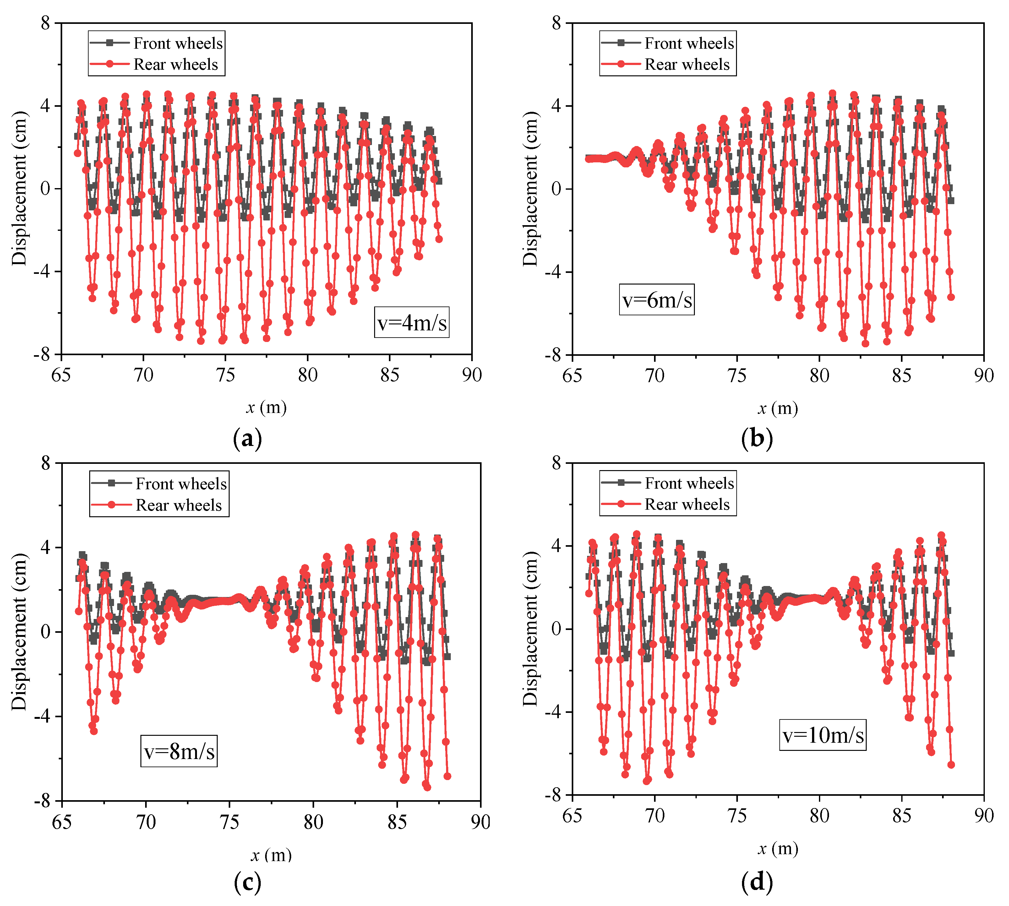
Figure 7 shows the net displacement and vertical acceleration calculated by Equation (26). The maximum net displacement difference is 5.95 cm at the front wheel and 12.1 cm at the rear wheel. When the front wheel drives on a flat road and the rear wheel is still on a bumpy road, the displacement near the rear wheel position is still large. The net vertical acceleration of the front and rear wheels is more than 3.2 m/s², the peak net acceleration of the rear wheels is 5.42 m/s², and the peak acceleration of the front wheels is 3.28 m/s². The rear wheel acceleration is generally higher than the front wheels. This means that the rear wheels are still bumpier at the road condition II.

4. Mechanical Responses of Bus in Driving under the Coupling Effect of Speed and Uneven Road Surface

With the increasing number of private cars, urban traffic becomes more and more crowded, and the speed of buses is getting slower and slower. Barabino et al. [43] conducted an experimental study on the bus driving conditions in the city of Cagliari, located in Sardinia (Italy). The original data of the bus driving are listed in

Table 2. Location-at-time raw data sample gathered by the app Torque on Tue Jul 2018 [43].

GPS Time	Longitude [°]	Latitude [°]	GPS Speed [m/s]	alat [m/s2]	along [m/s2]
10:33:55	9.10102	39.241895	4.01	−0.7346	−0.4840
10:33:56	9.101006667	39.24183833	4.50	−1.0937	0.5383
10:33:57	9.100983333	39.24177833	5.06	0.9893	−0.2925
10:33:58	9.100963333	39.24165	5.61	0.7977	−0.1417
10:33:59	9.100926667	39.24165	6.08	−0.1169	0.1289
10:34:00	9.10092	39.24158667	6.43	−0.7346	0.1193
10:34:01	9.100905	39.241525	6.68	0.1896	−0.4098

Note: a_lat means the acceleration component in latitude and a_long means the acceleration component in longitude.

. The speed of buses in rural regions is much faster than that in urban areas, so the four groups of buses selected in this section run at the speed of 4 m/s, 6 m/s, 8 m/s, and 10 m/s, respectively. Their mechanical responses when passing through the uneven road surface will be discussed below.

4.1. Road Condition I

The sketch of road conditions for the bus is shown in Figure 3. The front wheel drives into the uneven road section, but the rear wheel is still in the flat road section. The bus travel distance is 0 ≤ x ≤ (b + c). The net displacement of the front and rear wheels of the bus at this point is presented in Figure 8. When the speed is relatively high, the maximum net displacement be reached quicker. This means that the net displacement of the bus is smaller when the bus speed is slower. Thus, a greater bus speed will generate bigger net displacement. Therefore, a bus running at low speed has smaller displacement and higher passenger comfort. Figure 9 shows the acceleration change of the bus at different speeds. The acceleration also shows that when the bus speed is low, it takes longer to reach the maximum net acceleration of the vehicle, which means that the acceleration changes less at low speed, and the passenger comfort is higher.

Table 3. Maximum net displacement and acceleration of front and rear wheels at different speeds.

Velocity [m/s]	Front Wheel Displacement [cm]	Rear Wheel Displacement [cm]	Front Wheel Acceleration [m/s2]	Rear Wheel Acceleration [m/s2]
4	5.74	11.38	2.66	5.33
6	5.94	11.84	2.78	5.58
8	5.96	11.86	2.79	5.58
10	5.99	11.92	2.82	5.59

summarizes the maximum net displacement and acceleration at the front and rear wheels of the bus at different speeds. The net displacement basically does not change with speed and is mainly induced by road incentives. When the speed is low, both maximum net displacement and acceleration are still small, although the gap is small. However, it can be clearly observed from Figure 9 that the faster the speed is, the faster the bus reaches its maximum acceleration. This indicates that the higher the bus speed is, the longer the higher acceleration is maintained.

4.2. Road Condition II

Both the front and rear wheels drive into an uneven road section. At this time, the bus position is (b + c) ≤ x ≤ 2ns (n ∈ N*). N* is a positive integer. The net displacement and the net acceleration at different speeds are presented in Figure 10 and Figure 11, respectively.

Figure 10 shows the displacement of the bus in the middle section. It clearly shows that there is only one wave peak in (a), one and a half wave peaks in (b), and two wave peaks in (c), but the results are not obvious, while there are two wave peaks in (d). This means that faster speed will generate a higher frequency of large displacement. Figure 10c has obvious fluctuations, which are different from the other three figures. This mainly reflects the large displacement in a short time. This may be because the bus resonates with the ground when v = 8 m/s, resulting in the continuous large displacement of the whole bus.

The change in acceleration still shows that the comfort of the bus will be further reduced when the speed is fast. The change in v = 8 m/s is the most dramatic. At this time, the resonance situation does occur when the bus passes through the section (b + c) ≤ x ≤ 2ns (n ∈ N*), the comfort of passengers is the worst, and the overall displacement of the bus is the largest.

Table 4. Maximum net displacement and acceleration of front and rear wheels at different speeds.

Velocity [m/s]	Front Wheel Displacement [cm]	Rear Wheel Displacement [cm]	Front Wheel Acceleration [m/s2]	Rear Wheel Acceleration [m/s2]
4	2.65	2.35	0.05	0.08
6	2.39	2.68	0.12	0.19
8	4.20	5.45	0.65	1.23
10	3.31	3.63	0.25	0.41

records the maximum net displacement and acceleration corresponding to different speeds during the whole bus driving in road condition II. The overall acceleration changes uniformly and the displacement changes slightly when the bus passes through this section. When the bus speed is 8 m/s, both net displacement and net acceleration reach a maximum value of a sharp increase. This indicates that the resonance phenomenon between the bus and the road occurs at this time, and the passenger comfort is the lowest.

4.3. Road Condition III

The front wheel drives into the flat section, but the rear wheel is still in the uneven section. At this time, the bus position is 2ns ≤ x ≤ 2ns + (b + c) (n ∈ N*). The net displacement and net acceleration at different speeds are presented in Figure 12 and Figure 13, respectively. The calculation results in Figure 12 show that the bus has a small net displacement at the beginning when the bus is climbing at a speed of v = 6 m/s. This happens when the net displacements of the front and rear wheels are basically identical, and the spring is near the origin when the second section of the road is approaching the end.

Figure 12c,d and Figure 13 show that the springs of the front and rear wheels of the bus are in a tensile state before climbing, so there will be a very small displacement for a short period of time, then the spring will be compressed rapidly under the impact, and then repeated tensile compression will occur. Therefore, this phenomenon still means that when the bus is climbing a slope, slowing down is still the wisest choice, which will slow down the large instantaneous impact of the spring. A lower speed means that the passenger’s comfort is improved. The acceleration in Figure 13 shows that at different speeds, the acceleration undergoes a process of increasing from large to small, and then increasing. However, faster speeds will result in more wave crests and a more intense frequency of acceleration changes.

Table 5. Maximum net displacement and acceleration of front and rear wheels at different speeds.

Velocity [m/s]	Front Wheel Displacement [cm]	Rear Wheel Displacement [cm]	Front Wheel Acceleration [m/s2]	Rear Wheel Acceleration [m/s2]
4	5.97	11.93	2.76	5.24
6	5.97	12.06	2.76	5.25
8	5.94	11.96	2.75	5.22
10	5.91	11.91	2.74	5.51

records the maximum net displacement and acceleration corresponding to different speeds during the whole bus driving in road condition III. The maximum net displacement and acceleration of the bus at different speeds are basically the same when the bus is climbing. The reason is that the center of gravity of the bus is 2/3 away from the front wheel, and the excitation generated during climbing only has a large impact on the front wheel. The rear wheel should be kept in the motion state of road condition II at first, and then changed. The change is more drastic for greater speeds (see Figure 12c,d and Figure 13).

5. Mechanical Responses of Bus in Driving under the Coupling of Spring Stiffness and Uneven Pavement

For the completeness of the theoretical analysis, this section will discuss the mechanical response of the bus under three different coefficient ratios. The coefficient ratio of these three groups will take 1 as the boundary, and one group will be selected before and after each. The bus speed is given as a constant 6 m/s, and the grouping of stiffness coefficients is listed in

Table 6. The values of stiffness coefficient grouping.

Position	Low Ratio	Medium Ratio	High Ratio
Front wheel [N/m]	150,000	150,000	100,000
Rear wheel [N/m]	100,000	150,000	150,000

. The low ratio means that the stiffness coefficient is larger at the front wheel than at the rear wheel. The medium ratio means both the front and rear wheels have the same stiffness coefficient. The high ratio means that the stiffness coefficient is smaller at the front wheel than at the rear wheel.

5.1. Road Condition I

The front wheel drives into the uneven road section, but the rear wheel is still in the flat road section, and the bus travel distance is 0 ≤ x ≤ (b + c). In the case of road condition I, the displacement and acceleration changes of the front and rear wheels with different stiffness coefficient ratios are shown in Figure 14. The displacement changes little under different stiffness coefficient ratios. When the stiffness ratio is medium, the net displacement of the front and rear wheels is the minimum. The acceleration in Figure 14 obviously shows that the envelope of the black line can include all the curves. This means that the bus with low spring stiffness will cause a large acceleration change when the bus goes downhill.

5.2. Road Condition II

Both the front and rear wheels drive into an uneven road section, the bus position is (b + c) ≤ x ≤ 2ns (n ∈ N*). N* is a positive integer. In the case of road condition II, the displacement and acceleration of the front and rear wheels with different spring stiffness coefficient ratios are shown in Figure 15.

It is observed that the displacement is not obvious under different stiffness ratios. This may be that the slope is too small compared with the bus, and the front and rear wheels of the bus basically go up and down the slope synchronously. In the front wheel acceleration analysis in Figure 15, the low stiffness ratio means a large acceleration change, while the high stiffness ratio means a small change range. On the rear wheel acceleration, the change of the rear wheel of the bus is relatively small when the stiffness ratio is high. In other cases, the acceleration change is large.

5.3. Road Condition III

The front wheel drives into the flat section, but the rear wheel is still in the uneven section. At this time, the bus position is 2ns ≤ x ≤ 2ns + (b + c) (n ∈ N*). In the case of road condition III, the changes in displacement and acceleration at the front and rear wheels with different stiffness coefficient ratios are shown in Figure 16. The displacement changes are similar regardless of the stiffness coefficient ratio. The envelope of the black line can include all the curves about acceleration analysis in Figure 16. This implies that the curve with lower stiffness will lead to greater acceleration change when the bus goes uphill.

6. Conclusions

In this paper, from the perspective of rigid body dynamics, a motion differential equation suitable for bus driving was established by building a bumpy excitation road surface, and the mechanical response of the entire process on the road was analyzed. Secondly, based on the speed of the bus, the displacement and acceleration changes at different speeds were studied. Finally, the stiffness ratio of the front and rear wheels of the bus was analyzed. From these studies, the following conclusions can be drawn:

(1) When a bus travels on uneven roads, the rear seats are more bumpy than the front seats. The reason for this phenomenon is that the center of gravity of the bus is closer to the rear wheels, the rear wheels bear more force and are more prone to displacement. This indicates that bus design should pay special attention to the damping of the bus backseat and control its displacement. Passengers who are “old, weak, disabled, pregnant”, especially elderly people with osteoporosis, should avoid the seats at the rear of the bus as much as possible.

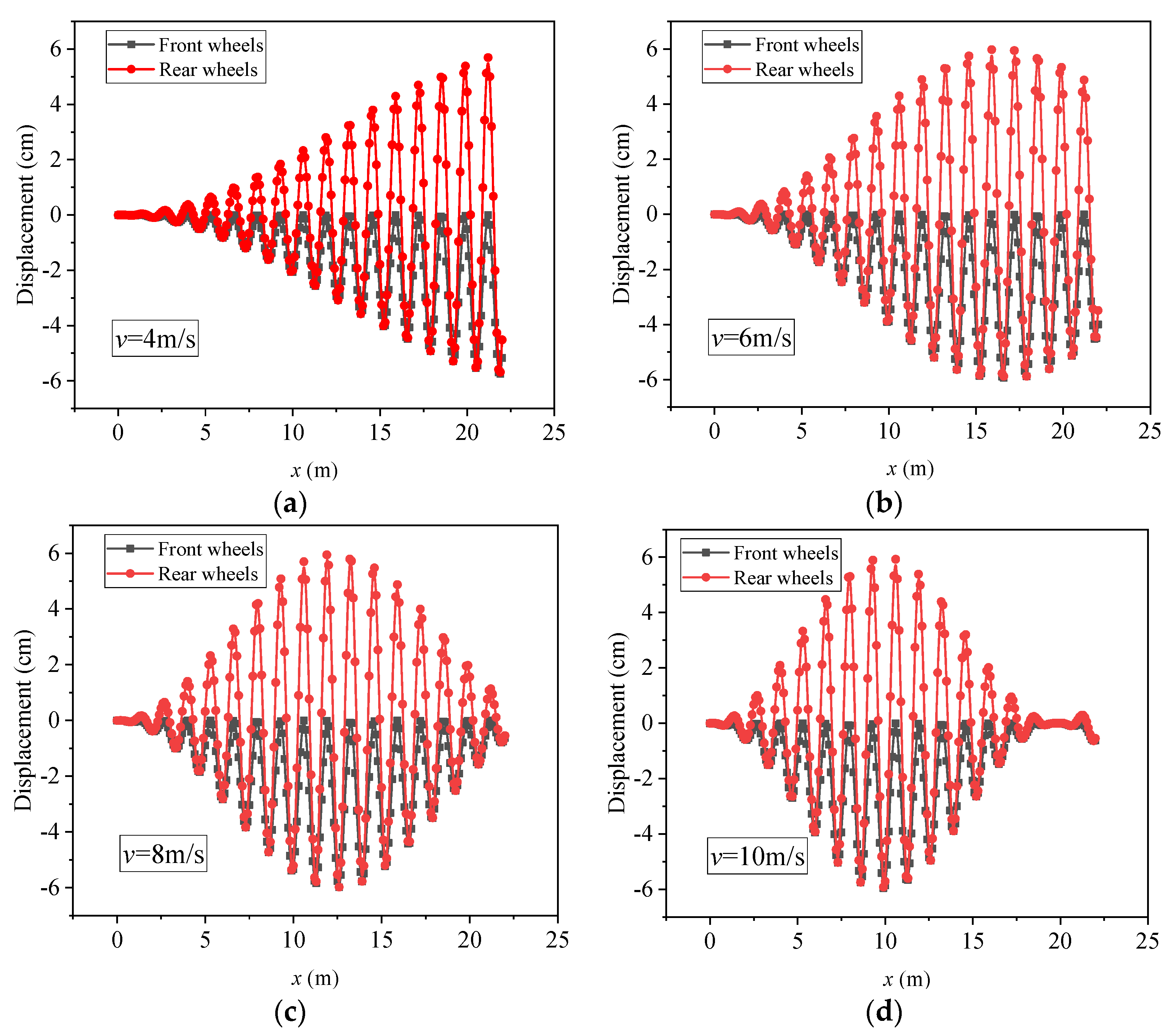
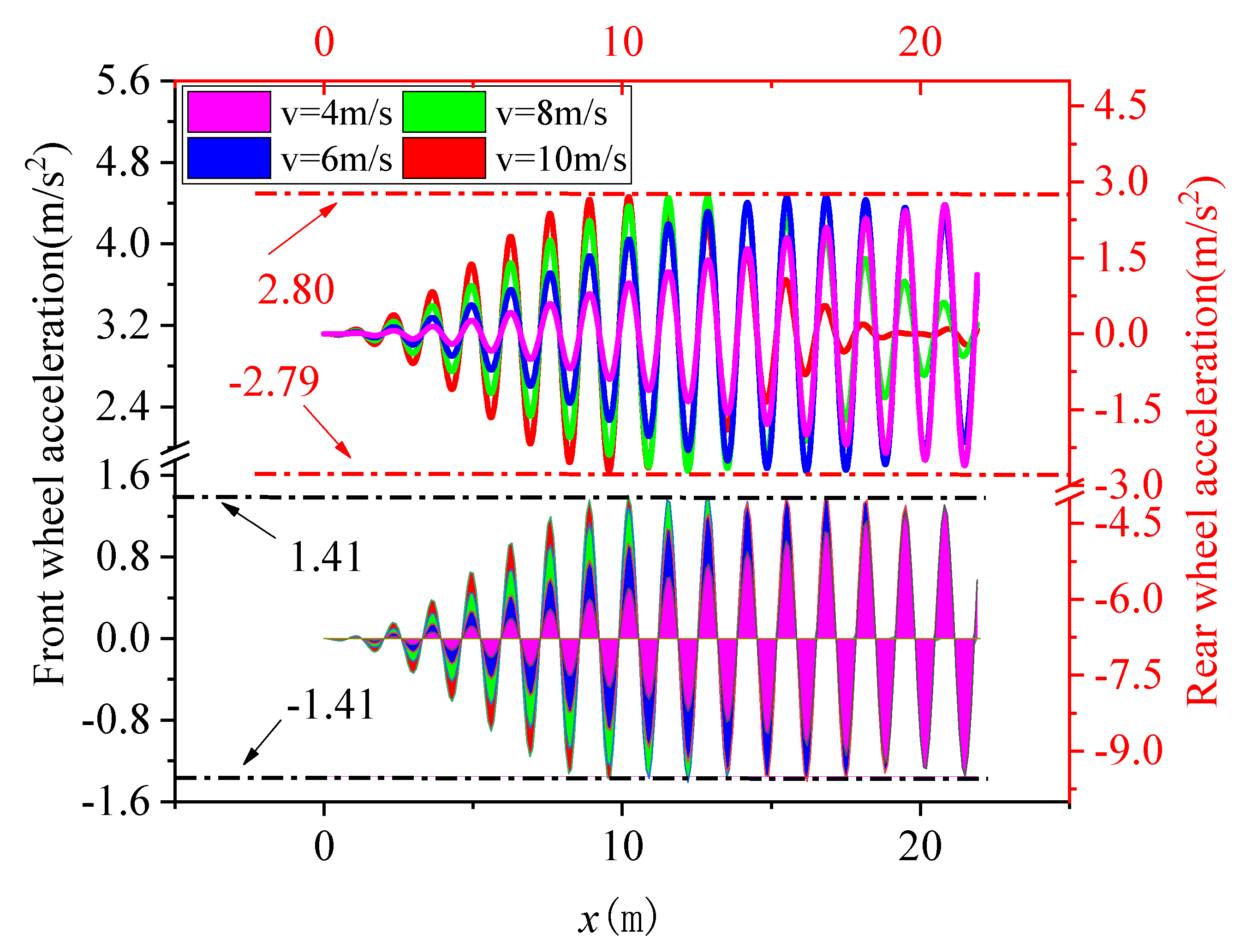
(2) The bus should not drive too fast on uneven roads. For the simplified bus model and excitation pavement discussed in this paper, faster speed means higher displacement and acceleration variation, which is not conducive to passenger comfort. Regardless of the speed, similar displacements and accelerations will ultimately be achieved, but the speed is higher, and the duration of maximum displacement and acceleration is longer.

(3) The spring stiffness ratio of the bus indicates that the bus is more stable when the rear wheels are high in spring stiffness. A bus model with low stiffness, whether climbing or downhill, will produce significant acceleration changes. During the manufacturing process of cars, it is better to ensure that the rear wheels have a higher stiffness coefficient, while appropriately reducing the stiffness of the front wheels.

The results of this paper have certain significance. Engineers can use the differential equations and analytical solutions in this paper to roughly analyze the mechanical response of a moving bus by establishing an actual excitation road surface. These results can provide some guidance for the design and driving of buses. However, the impact of damping has been ignored in this paper. Damping can be taken into account in future bus models to more accurately analyze the mechanical response of buses during driving.

References

1. Kuys, J.; Melles, G.; Al Mahmud, A.; Thompson-Whiteside, S.; Kuys, B. Human centred design considerations for the development of sustainable public transportation in Malaysia. Appl. Sci. 2022, 12, 12493. [Google Scholar] [CrossRef]
2. Coermann, R.R. The mechanical impedance of the human body in sitting and standing position at low frequencies. Hum. Factors 1962, 4, 227–253. [Google Scholar] [CrossRef]
3. Gao, J.H.; Hou, Z.C.; He, L.; Xia, Q.S. Vertical vibration characteristics of seated human bodies and a biodynamic model with two degrees of freedom. Sci. China Technol. Sci. 2011, 54, 2776–2784. (In Chinese) [Google Scholar] [CrossRef]
4. Bazil, B.; Griffin, M.J. Equivalent comfort contours for vertical seat vibration: Effect of vibration magnitude and backrest inclination. Ergonomics 2012, 55, 909–922. [Google Scholar]
5. Xie, W.P.; Zhang, H.; He, W. Field measurement for vehicle induced vibration of a multi-story 3-D bus station. J. Vib. Shock 2020, 39, 138–245. (In Chinese) [Google Scholar]
6. Zhou, Z.; Griffin, M.J. Response of the seated human body to whole-body vertical vibration: Discomfort caused by sinusoidal vibration. Ergonomics 2014, 57, 714–732. [Google Scholar] [CrossRef] [PubMed] [Green Version]
7. Oboknb, D.J.; Clarke, M.J. The development of questionnaire surveys for the investigation of passenger comfort. Ergonomics 1973, 16, 855–869. [Google Scholar] [CrossRef]
8. EN 13816; Transportation-Logistics and Services, European Standard EN 13816: Public Passenger Transport-Service Quality Definition, Targeting and Measurement. EN: Washington, DC, USA, 2002.
9. Prashanth, A.S.; Saran, V.H.; Harsha, S.P. December. Study of subjective responses on ride comfort in public transport Uttarakhand State buses. In Proceedings of the 1st International and 16th National Conference on Machines and Mechanisms (iNaCoMM), Roorkee, India, 18–20 December 2013; pp. 1–5. [Google Scholar]
10. Zhang, K.; Zhou, K.; Zhang, F. Evaluating bus transit performance of Chinese cities: Developing an overall bus comfort model. Transp. Res. Part A Policy Pract. 2014, 69, 105–112. [Google Scholar] [CrossRef]
11. das Neves Almeida, M.; de Paula Xavier, A.A.; Michaloski, A.O. A review of thermal comfort applied in bus cabin environments. Appl. Sci. 2020, 10, 8648. [Google Scholar] [CrossRef]
12. Kilikevičius, A.; Kilikevičienė, K.; Matijošius, J. Investigation of drivers’ comfort factors influencing urban traffic safety. In Vision Zero for Sustainable Road Safety in Baltic Sea Region, Proceedings of the International Conference “Vision Zero for Sustainable Road Safety in Baltic Sea Region”, Vilnius, Lithuania, 5–6 December 2018; Springer International Publishing: Berlin/Heidelberg, Germany, 2020; pp. 159–165. [Google Scholar]
13. Zhou, X.; Liu, Y.; Luo, M.; Zheng, S.; Yang, R.; Zhang, X. Overall and thermal comfort under different temperature, noise, and vibration exposures. Indoor Air 2022, 32, e12915. [Google Scholar] [CrossRef]
14. Mathes, M.; Schmidt, M.; Käsgen, J.; Fievet, B.; Tichelen, P.V.; Berecibar, M.; Al-Saadi, M. Heavy-duty battery electric buses’ integration in cities based on superfast charging technologies: Impact on the urban life. Sustainability 2022, 14, 4777. [Google Scholar] [CrossRef]
15. Lin, C.Y.; Chen, L.J.; Chen, Y.Y.; Lee, W.C. A comfort measuring system for public transportation systems using participatory phone sensing. ACM Phonesense 2010. Available online: https://www.iis.sinica.edu.tw/papers/cclljj/11583-F.pdf (accessed on 4 March 2023).
16. Wåhlberg, A.E.A. Short-term effects of training in economical driving: Passenger comfort and driver acceleration behavior. Int. J. Ind. Ergon. 2006, 36, 151–163. [Google Scholar] [CrossRef]
17. Lin, C.Y.; Chen, L.J. TPE-CMS: A comfort measuring system for public bus service in Taipei city. In Proceedings of the International Conference on Computer Communication, Nagpur, Maharashtra, India, 21–22 April 2011. [Google Scholar]
18. EN 12299; Railway Applications: Ride Comfort for Passengers—Measurement and Evaluation. EN: Washington, DC, USA, 2009.
19. Sekulić, D.; Dedović, V.; Rusov, S.; Šalinić, S.; Obradović, A. Analysis of vibration effects on the comfort of intercity bus users by oscillatory model with ten degrees of freedom. Appl. Math. Model. 2013, 37, 8629–8644. [Google Scholar] [CrossRef]
20. Sekulić, D.; Dedović, V.; Rusov, S.; Obradović, A.; Šalinić, S. Definition and determination of the bus oscillatory comfort zones. Int. J. Ind. Ergon. 2016, 53, 328–339. [Google Scholar] [CrossRef]
21. Sekulić, D.; Rusov, S.; Dedović, V.; Šalinić, S.; Mladenović, D.; Ivković, I. Analysis of bus users’ vibration exposure time. Int. J. Ind. Ergon. 2018, 65, 26–35. [Google Scholar] [CrossRef]
22. Castellanos, J.C.; Fruett, F. Embedded system to evaluate the passenger comfort in public transportation based on dynamical vehicle behavior with user’s feedback. Measurement 2014, 47, 442–451. [Google Scholar] [CrossRef]
23. Maternini, G.; Cadei, M. A comfort scale for standing bus passengers in relation to certain road characteristics. Transp. Lett. 2014, 6, 136–141. [Google Scholar] [CrossRef]
24. Sekulić, D.; Mladenović, D. Evaluation and analysis of vibration effects on bus users. ЗБОРНИК НА ТРУДОВИ 2016, 342, 435–444. [Google Scholar]
25. Vovsha, P.; Oliveira, M.G.S.; Davidson, W.; Chu, C.; Farley, R.; Mitchell, M.; Vyas, G. Statistical analysis of transit user preferences including in-vehicle crowding and service reliability. In Proceedings of the Transportation Research Board 93rd Annual Meeting, Washington, DC, USA, 12–16 January 2014. [Google Scholar]
26. Zhao, H.; Guo, L.L.; Zeng, X.Y. Evaluation of bus vibration comfort based on passenger crowdsourcing mode. Math. Probl. Eng. 2016, 2016, 2132454. [Google Scholar] [CrossRef] [Green Version]
27. Eboli, L.; Mazzulla, G.; Pungillo, G. Measuring bus comfort levels by using acceleration instantaneous values. Transp. Res. Procedia 2016, 18, 27–34. [Google Scholar] [CrossRef]
28. Shen, X.; Feng, S.; Li, Z.; Hu, B. Analysis of bus passenger comfort perception based on passenger load factor and in-vehicle time. SpringerPlus 2016, 5, 62. [Google Scholar] [CrossRef] [PubMed] [Green Version]
29. Barabino, B.; Eboli, L.; Mazzulla, G.; Mozzoni, S.; Murru, R.; Pungillo, G. An innovative methodology to define the bus comfort level. Transp. Res. Procedia 2019, 41, 461–470. [Google Scholar] [CrossRef]
30. Meiping, Y.; Wen, W.A.N.G. Smartphone based research of measurement indexes related to bus riding comfort. J. Tongji Univ. (Nat. Sci.) 2017, 45, 1143–1149. [Google Scholar]
31. Nguyen, T.; NguyenDinh, N.; Lechner, B.; Wong, Y.D. Insight into the lateral ride discomfort thresholds of young-adult bus passengers at multiple postures: Case of Singapore. Case Stud. Transp. Policy 2019, 7, 617–627. [Google Scholar] [CrossRef]
32. Wang, G.; Zhang, J.; Kong, X. Study on passenger comfort based on human–bus–road coupled vibration. Appl. Sci. 2020, 10, 3254. [Google Scholar] [CrossRef]
33. Bae, I.; Moon, J.; Seo, J. Toward a comfortable driving experience for a self-driving shuttle bus. Electronics 2019, 8, 943. [Google Scholar] [CrossRef] [Green Version]
34. Nguyen, T.; Nguyen-Phuoc, D.Q.; Wong, Y.D. Developing artificial neural networks to estimate real-time onboard bus ride comfort. Neural Comput. Appl. 2021, 33, 5287–5299. [Google Scholar] [CrossRef]
35. Szumska, E.M.; Stańczyk, T.L.; Zuska, A.; Grabski, P.; Jaśkiewicz, M.; Jurecki, R.; Kurczyński, D.; Łagowski, P. Experimental testing of longitudinal acceleration in urban buses. In IOP Conference Series: Materials Science and Engineering; IOP Publishing: Bristol, UK, 2022; Volume 1247, p. 012017. [Google Scholar]
36. Zhang, G.X.; Ye, D. Eleven DOF vehicle dynamics model and comfort simulation. Mach. Des. Manuf. 2017, 1, 43–46. (In Chinese) [Google Scholar]
37. Tang, C.; Zhang, T.; Li, H.; Zhou, W. Evaluation of ride comfort of a vehicle. J. Vib. Shock 2009, 27, 158–166. (In Chinese) [Google Scholar]
38. Bogsjö, K.; Podgórski, K.; Rychlik, I. Models for road surface roughness. Veh. Syst. Dyn. 2012, 50, 725–747. [Google Scholar] [CrossRef]
39. Chen, Z.; Liang, Y.; Xue, B.; Sun, L. Relationship between vehicle vibration characteristics and human ride comfort. J. Tongji Univ. (Nat. Sci.) 2020, 48, 1007–1015. (In Chinese) [Google Scholar]
40. Agostinacchio, M.; Ciampa, D.; Olita, S. The vibrations induced by surface irregularities in road pavements—A Matlab approach. Eur. Transp. Res. Rev. 2014, 6, 267–275. [Google Scholar] [CrossRef] [Green Version]
41. Wu, J.; Hao, L. Why the rear row of a big car bumps more than the front row. Mech. Eng. 2008, 30, 102–103. (In Chinese) [Google Scholar]
42. Song, X.Z. The complementarity of “Why back row seats of a bus are more jolty”. Mech. Eng. 2008, 30, 115. (In Chinese) [Google Scholar]
43. Barabino, B.; Coni, M.; Olivo, A.; Pungillo, G.; Rassu, N. Standing passenger comfort: A new scale for evaluating the real-time driving style of bus transit services. IEEE Trans. Intell. Transp. Syst. 2019, 20, 4665–4678. [Google Scholar] [CrossRef]
44. Nguyen, T.; Swolana, P.; Lechner, B. An experimental comparison of mathematical heavy-duty city bus models to evaluate passenger ride comfort induced by road roughness. Math. Comput. Model. Dyn. Syst. 2021, 27, 203–221. [Google Scholar] [CrossRef]
45. Zhang, H.; Li, X.; Zheng, X.; Liu, H. Analysis of bus maneuverability and stability impact elements based on MATLAB. In Proceedings of the 2010 International Conference on Intelligent Computation Technology and Automation, Changsha, China, 11–12 May 2010; Volume 1, pp. 647–650. [Google Scholar]
46. Kong, Y.S.; Omar, M.Z.; Chua, L.B.; Abdullah, S. Ride quality assessment of bus suspension system through modal frequency response approach. Adv. Mech. Eng. 2014, 6, 269721. [Google Scholar] [CrossRef] [Green Version]
47. Long, L.X.; Quynh, L.V.; Cuong, B.V. Study on the influence of bus suspension parameters on ride comfort. Vibroeng. Procedia 2018, 21, 77–82. [Google Scholar] [CrossRef] [Green Version]
48. Olmeda, E.; Li, E.R.C.; Hernández, J.R.; Díaz, V. Lateral dynamic simulation of a bus under variable conditions of camber and curvature radius. Mathematics 2022, 10, 3081. [Google Scholar] [CrossRef]
49. Mei, F.X. On D’Alembert’s Principle—The Sixth Reading Notes of Theoretical Mechanics. Mech. Eng. 2009, 31, 61–63. (In Chinese) [Google Scholar]
50. Bus Network. Yutong ZK6105HNGS1 Bus Model Parameters. [EB/OL]. Available online: https://www.chinabuses.com/product/buses/8066.html (accessed on 1 December 2022).
51. Xu, J.; Yang, K.; Luo, Q.; Shao, Y. Field measurement of automobiles’ lateral accelerations. J. Southwest Jiaotong Univ. 2014, 27, 536–545. (In Chinese) [Google Scholar]
52. Zhang, J.; Wang, G.; Ji, Z.; Wang, Y.; Zhang, S. Comfort analysis of large bus considering the effect of braking force. Chin. J. Appl. Mech. 2020, 2, 777–784. (In Chinese) [Google Scholar]
53. Cheng, Y.; Li, X.; Sun, S.; Man, X.; Fan, F.; Li, Z. A new method for expression and classification of long wave road surface unevenness in field. J. Vib. Shock. 2022, 11, 41. (In Chinese) [Google Scholar]
54. Liu, L.; Zhang, Z.; Lu, H.; Xu, Z. Road roughness identification based on augmented kalman filtering with consideration of vehicle acceleration. Automot. Eng. 2022, 44, 247–255, 297. (In Chinese) [Google Scholar]
55. Wang, H. Research on the identification of rural highway deformation diseases based on pavement smoothness index. Sino-Foreign Highw. 2022, 42, 78–82. (In Chinese) [Google Scholar]
56. Zhang, J.L.; Chen, R.F.; Yao, K. Analysis on influence of road pavement roughness on vehicle vibration. J. Highw. Transp. Res. Dev. 2019, 36, 129–133. (In Chinese) [Google Scholar]
57. Li, W.; Wang, G. Vehicle ride comfort analysis based on bridge deck with irregular pavement. J. Beijing Jiaotong Univ. 2022, 46, 98–104. (In Chinese) [Google Scholar]
Figure 1. Force model of a bus in general driving conditions.
Applsci 13 04639 g001
Figure 2. Relationship between ground support forces on front and rear wheels and acceleration.
Applsci 13 04639 g002
Figure 3. A simplified mechanical analysis of uneven pavement.
Applsci 13 04639 g003
Figure 4. Sketch of the force analysis of the upper part of the bus.
Applsci 13 04639 g004
Figure 5. Net displacement (a) and vertical acceleration (b) of front and rear wheels 0x ≤ (b + c).
Applsci 13 04639 g005
Figure 6. Net displacement (a) and vertical acceleration (b) of front and rear wheels (b + c) ≤ x ≤ 2ns (nN*).
Applsci 13 04639 g006
Figure 7. Net displacement (a) and vertical acceleration (b) of front and rear wheels 2nsx ≤ 2ns + (b + c) (nN*).
Applsci 13 04639 g007
Figure 8. Net displacement of front and rear wheels 0x ≤ (b + c): (a) v = 4 m/s; (b) 6 m/s; (c) 8 m/s; (d) 10 m/s.
Applsci 13 04639 g008
Figure 9. Net vertical acceleration of front and rear wheels at different speeds 0 ≤ x ≤ (b + c).
Applsci 13 04639 g009
Figure 10. Net displacement of front and rear wheels (b + c) ≤ x ≤ 2ns (nN*): (a) v = 4 m/s; (b) 6 m/s; (c) 8 m/s; (d) 10 m/s.
Applsci 13 04639 g010
Figure 11. Net vertical acceleration of front and rear wheels at different speeds (b + c) ≤ x ≤ 2ns (nN*).
Applsci 13 04639 g011
Figure 12. Net displacement of front and rear wheels 2nsx ≤ 2ns + (b + c) (nN*): (a) v = 4 m/s; (b) 6 m/s; (c) 8 m/s; (d) 10 m/s.
Applsci 13 04639 g012
Figure 13. Net vertical acceleration of front and rear wheels at different speeds 2nsx ≤ 2ns + (b + c) (nN*).
Applsci 13 04639 g013
Figure 14. Net displacement and vertical acceleration 0x ≤ (b + c) (The black line is the envelope of scattered points at low stiffness ratio; the red line is the envelope of scattered points at medium stiffness ratio; the blue line is the envelope of scattered points at high stiffness ratio).
Applsci 13 04639 g014
Figure 15. Net displacement and vertical acceleration (b + c) ≤ x ≤ 2ns (nN*) (The black line is the envelope of scattered points at low stiffness ratio; the red line is the envelope of scattered points at medium stiffness ratio; the blue line is the envelope of scattered points at high stiffness ratio).
Applsci 13 04639 g015
Figure 16. Net displacement and vertical acceleration 2nsx ≤ 2ns + (b + c) (nN*) (The black line is the envelope of scattered points at low stiffness ratio; the red line is the envelope of scattered points at medium stiffness ratio; the blue line is the envelope of scattered points at high stiffness ratio).
Applsci 13 04639 g016