
A Vision Detection Scheme Based on Deep Learning in a Waste Plastics Sorting System
1
The Key Laboratory of Polymer Processing Engineering of Ministry of Education, South China University of Technology, Guangzhou 510641, China
2
Guangdong Provincial Key Laboratory of Technique and Equipment for Macromolecular Advanced Manufacturing, South China University of Technology, Guangzhou 510641, China
3
School of Mechanical and Automotive Engineering, South China University of Technology, Guangzhou 510641, China
*
Author to whom correspondence should be addressed.
Appl. Sci. 2023, 13(7), 4634; https://doi.org/10.3390/app13074634
Submission received: 14 March 2023
/
Revised: 31 March 2023
/
Accepted: 4 April 2023
/
Published: 6 April 2023
(This article belongs to the Section Applied Industrial Technologies)
Abstract
:The preliminary sorting of plastic products is a necessary step to improve the utilization of waste resources. To improve the quality and efficiency of sorting, a plastic detection scheme based on deep learning is proposed in this paper for a waste plastics sorting system based on vision detection. In this scheme, the YOLOX (You Only Look Once) object detection model and the DeepSORT (Deep Simple Online and Realtime Tracking) multiple object tracking algorithm are improved and combined to make them more suitable for plastic sorting. For plastic detection, multiple data augmentations are combined to improve the detection effect, while BN (Batch Normalization) layer fusion and mixed precision inference are adopted to accelerate the model. For plastic tracking, the improved YOLOX is used as a detector, and the tracking effect is further improved by optimizing the deep cosine metric learning and the metric in the matching stage. Based on this, virtual detection lines are set up to filter and extract information to determine the sorted objects. The experimental results show that the scheme proposed in this paper makes full use of vision information to achieve dynamic and real-time detection of plastics. The system is effective and versatile for sorting complex objects.
1. Introduction
Plastic products are among the most common objects in daily life and one of the most valuable categories in waste recycling. Since plastics are macromolecule compounds made of monomers, polymerized by polymerization or polycondensation reactions, they are difficult to degrade by themselves under natural conditions and are difficult to dispose of harmlessly. However, the dramatic increase in plastic waste has seriously affected the natural environment and human life, so the management of waste plastics is crucial [1]. According to the OCDE report [2], the amount of plastic produced globally in 2019 was 460 million tons, and there were 353 million tons of plastic waste, of which packaging accounted for 40%. Waste plastics have more than doubled since 2000, but with only 9% recycled, plastic production is expected to keep growing. Therefore, it is of great significance to study efficient plastic recycling methods.
Before disposing of the recycled plastic, it should be sorted as needed to facilitate subsequent work. Manual sorting is labor-intensive, harsh, and inefficient. Traditional plastic sorting methods include density sorting [3], flotation [4], electrical sorting [5], wind sorting [6], near-infrared sorting [7], etc. This kind of method is suitable for a specific or single type of plastic and has limitations in sorting a large number of different waste plastic packaging with different categories and shapes. In order to improve efficiency and quality, machine vision systems are combined in the other industrial fields involving detection, and so vision detection technology has been widely used in the industry [8]. Compared with traditional methods, vision detection methods based on industrial cameras have advantages such as high efficiency and non-contact characteristics. Therefore, industrial cameras are currently one of the most widely used sensors and an essential component in image-processing systems [9]. Vision-based automated sorting provides an effective method for the recycling of waste plastics. The main research in this paper focuses on how to make full use of the visual information provided by the industrial camera to realize dynamic sorting when facing complex operational objects with different categories, locations, shapes, and heights.
To improve the accuracy and efficiency of plastic detection so as to provide accurate information for subsequent sorting, scholars have carried out a considerable amount of research in designing vision detection methods. The existing research is mainly divided into two types: the first is the traditional machine learning method, and the second is the method based on deep learning. The first type usually contains three main parts: data processing, feature extraction, and selecting machine learning algorithms as classifiers [10]. TORRES et al. binarized the acquired RGB images and then used Hu moment to extract a set of numerical attributes from the region of interest, and fed them into the k-NN classifier to realize the classification of plastic cutlery, plastic bottles, and aluminum cans [11]. OZKAN K et al. studied the classification of three plastics: PET, HPDE, and PP. Plastic regions were first extracted and morphological manipulations were performed. Then, the majority voting scheme combined with Principal Component Analysis (PCA), Kernel PCA (KPCA), Fisher’s Linear Discriminant Analysis (FLDA), Singular Value Decomposition (SVD), and Laplacian Eigenmaps (LEMAP) was used to extract features. Finally, the Support Vector Machine (SVM) was used for classification. The proposed method outperforms the single classifier [12]. PAULRAJ S G et al. proposed a robotic-arm sorting method based on a thermal imaging camera and proximity sensor. They adopted a SURF feature extractor to extract key points and fed them into clustering model for feature mapping. Finally, aluminum cans, plastic bottles, and Tetra Paks were sorted using the SVM classifier [13]. Wang et al. first used distance transformation, threshold segmentation, and other methods to process images. Then, the ReliefF algorithm was applied to select the color features of plastic bottles. Finally, the SVM was used for color classification [14]. Tan et al. first segmented the effective area of the plastic bottle. Then, the mean, the standard deviation, and the coefficient of variation of the approximate refractive index and intensity distributions were used to construct the feature. Finally, they used the SVM for the identification of PET plastic bottles [15]. The first type of method can achieve better sorting results in structured application scenarios where objects are relatively homogeneous in shape and regular in distribution, relying on preset processes and parameters. However, due to its low robustness, the manually designed feature extractor has limitations when the detection object or working environment is complex.
For the second type of detection method, the main difference between it and the first type is feature extraction. In contrast, deep learning can automatically extract features and has the ability to learn from large amounts of data. Therefore, it has significant advantages in image recognition and data processing [16]. Convolutional Neural Network (CNN) is the most commonly used deep learning technique. Owen Tamin et al. listed and discussed the application of classification models based on CNN in plastic waste detection [17]. For example, Srinilta et al. studied the performance of VGG16, ResNet50, MobileNet V2, and DenseNet121 for classifying municipal solid waste, and ResNet50 performed the best [18]. Zhang et al. added the self-monitoring module on the basis of ResNet18 to improve the model’s ability to classify different wastes [19]. Such methods rely on CNN to automatically extract features, and the accuracy rate can reach more than 85%. They address the limitations of the first type of method, and it is confirmed that deep learning can effectively extract the features of plastics and accurately classify them. However, the classification model can only predict one label each time. It is suitable for classification tasks that contain only a single object on each image [20].
In challenges with the need for both classification and localization, object detection based on deep learning is considered as an advanced solution [21]. Currently, object detection has been applied in many scenarios, such as defect detection [22], agricultural product detection [23], face detection [24], and automatic driving [25]. Ye et al. proposed a YOLOv1-based neural network model with Variational Autoencoder (VAE) for detecting recyclable waste such as cans, batteries, and plastic bottles [26]. Melinte et al. combined MobileNet and SSD for multiple waste detection [27]. Zhang et al. constructed a YOLO-WASTE multi-label waste classification model based on YOLOv4 to realize fast recognition and classification of multiple wastes, including waste glass, waste fabric, waste metal, waste plastic, and waste paper [28]. Mao et al. trained YOLOv3 on the dataset containing six categories—plastic containers, plastic bottles, metal, cartons, paper containers, and glass—for detecting domestic waste [29]. These efficient object detection models can be used to detect various types of waste. Therefore, this paper adopts object detection to output the category and location information of plastics. CHEN Z H et al. proposed a single-category detection method based on the Region Proposal Network (RPN) and VGG-16 model. The robotic arm grasped plastic bottles among multiple categories of waste conveyed by the conveyor belt according to the geometric center and long-side angle [30]. LEE S-H et al. proposed an embedded waste recycling method based on an SSD detector. A robotic arm received location and category information and sorted objects on an electronic rotating turntable [31]. Seredkin et al. proposed a solid waste sorting method based on Fast R-CNN. They used a height profile scanner to measure the height of the objects and sent the category, location, and height information to the robot to achieve sorting [32]. These methods confirm that object detection can effectively assist the robotic arm in sorting. However, for scenarios where the conveyor belt is applied, introducing new sensors to obtain more information increases the complexity of the system and sources of error.
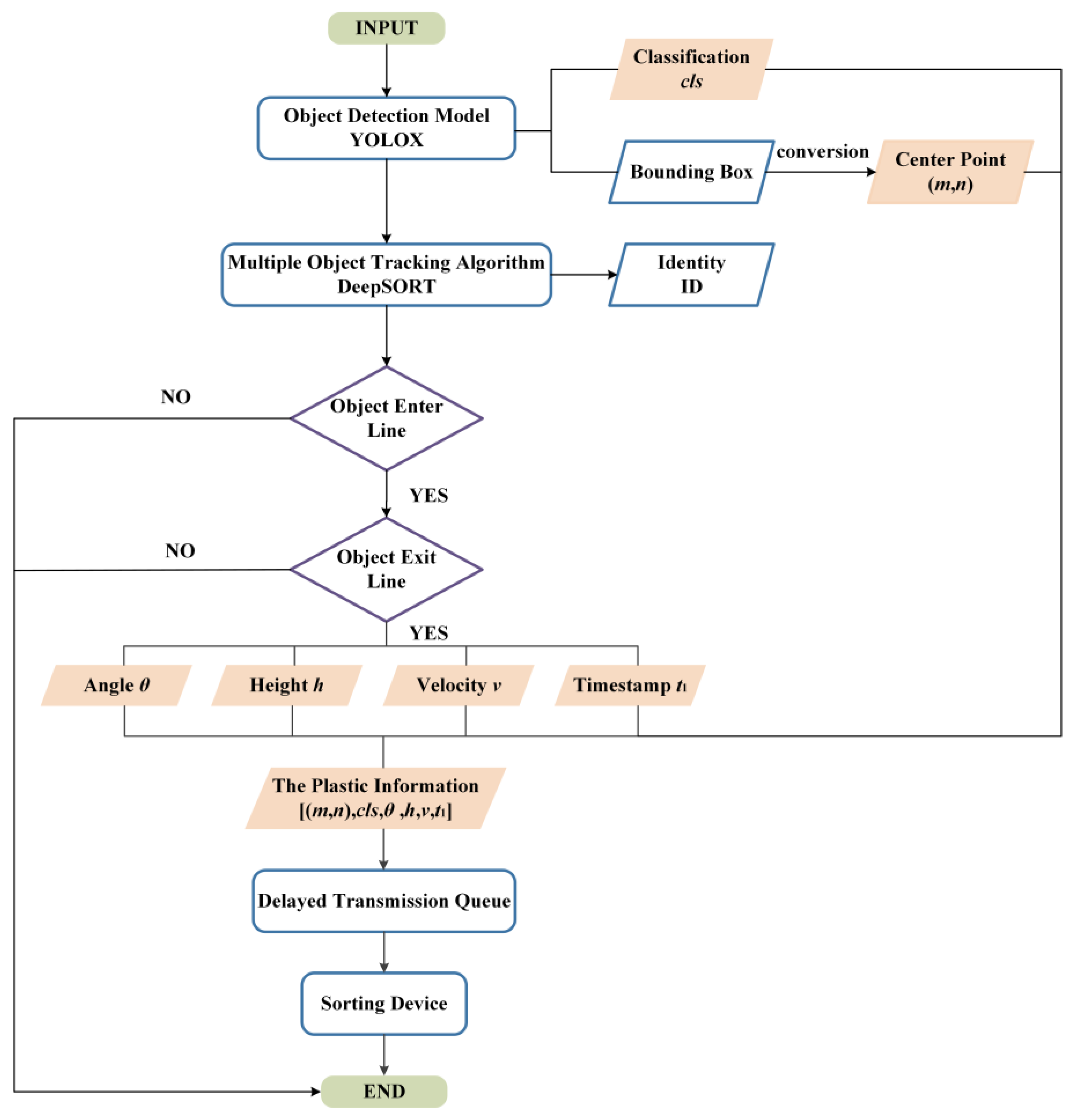
Furthermore, object detection processes the static single frame and does not correlate the detection results of the preceding and following frames. It is obviously not feasible to send all the information detected in the camera field of view directly to the sorting device. To solve this problem, multiple object tracking based on detection is introduced in this paper. This algorithm is commonly used for pedestrian tracking [33] and traffic flow detection [34]. Applying it to plastic detection can achieve deduplication and avoid unordered sorting. In addition, due to the different shapes and random postures of the waste plastics, it is necessary to obtain information about the height, angle, and velocity of the plastics to ensure the success of sorting. Based on the above analysis, this paper takes five common categories of plastics, such as wash supplies bottles, beverage bottles, Tetra Paks, express packages, and tableware boxes, as macroscopic sorting objects, and designs a multi-category dynamic sorting system based on visual guidance in unstructured scenes. Since the quality of the vision detection method directly affects the sorting performance of the system [35], this study focuses on the feasibility and effectiveness of the plastic detection method based on object detection and multiple object tracking. The process of the plastics detection algorithm is designed as shown in Figure 1.
The main contributions of this paper are as follows:
- 1.
- A plastic detection algorithm based on improved YOLOX [36]. The algorithm achieves a better trade-off between detection accuracy and inference speed. It classifies and localizes plastics by capturing appearance features.
- 2.
- A plastic tracking algorithm based on improved DeepSORT [37]. The algorithm performs tracking based on the output information of the detector. It transforms multiple object tracking into a problem of data association of detection results to achieve object deduplication.
- 3.
- An information acquisition method based on virtual two-line detection. The method combines the plastic detection algorithm and the plastic tracking algorithm. To save computational resources, two virtual detection lines are set up to constitute the plastic detection area for filtering and extracting relevant information. It realizes an efficient real-time dynamic detection method.
- 4.
- For the acquisition of plastic information, the combination of minimum bounding rectangle, image mask, and the topK algorithm to calculate the angle and height, using a Kalman filter for real-time filtering of velocity. The system is no longer external to other sensors, giving full play to the role and advantages of vision detection technology and improving the flexibility and versatility of the system.
The rest of this paper is organized as follows: Section 2 introduces the design of the vision detection system. Section 3 elaborates on the plastic detection method based on object detection and multiple object tracking, and describes the workflow of the system for detecting plastics. Section 4 gives the implementation and results of the experiments. Section 5 summarizes the whole paper.
2. System Overview
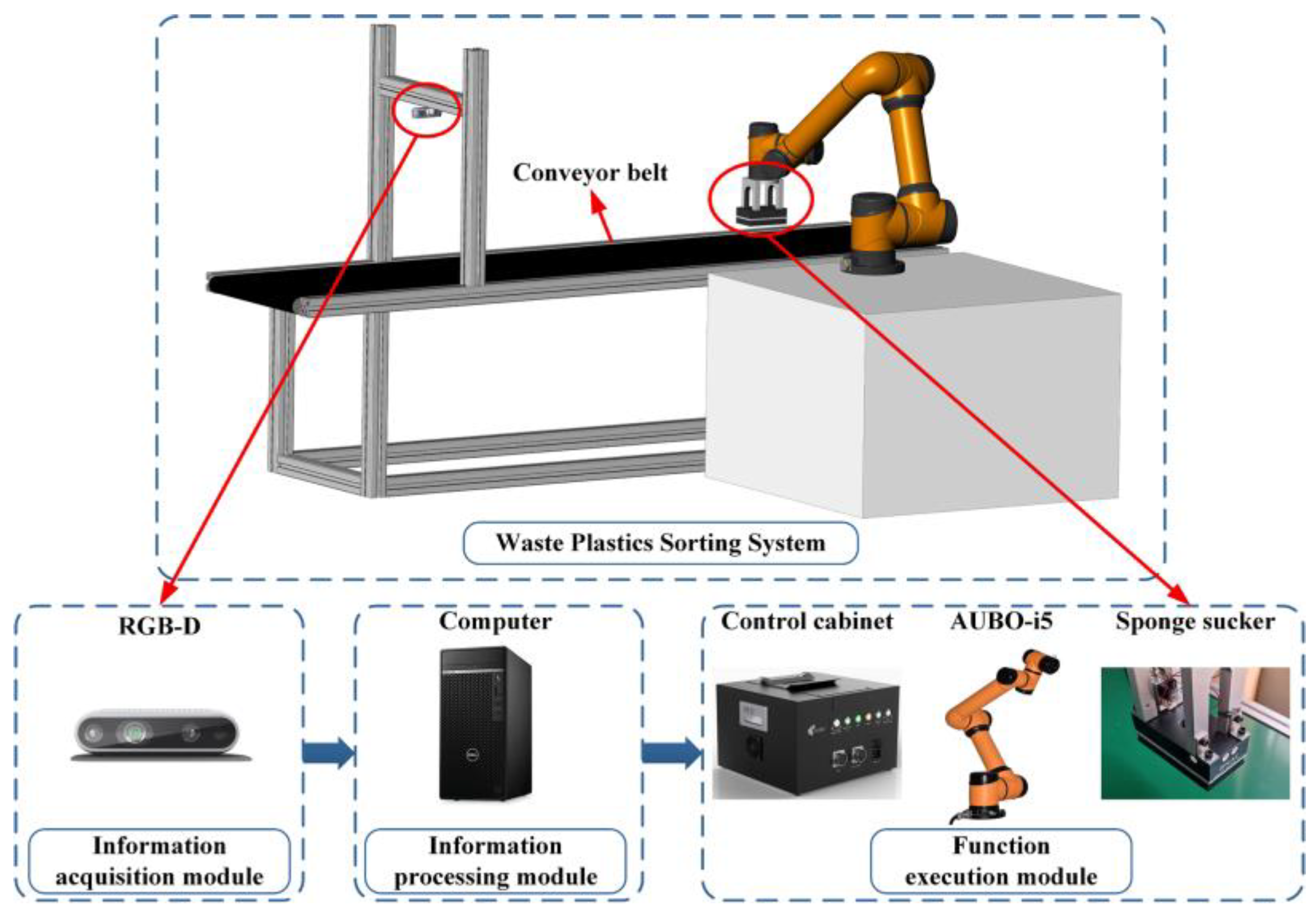
Figure 2 shows the waste plastics sorting system and the connection between the components. The whole system consists of four parts: the information acquisition module, the function execution module, the information processing module, and the conveyor module.
The information acquisition module adopts the Intel RealSense D435 depth camera, based on the combination of a single infrared structured light emitter, a binocular infrared camera, and a single color camera. The function execution module controls the robotic arm to complete the sorting action by receiving commands from the computer. The AUBO-i5 six degrees of freedom robotic arm is equipped with an AUBO-CB-M control cabinet. The end of the robotic arm is equipped with an integrated vacuum sponge sucker with a built-in vacuum generator, which can suck the object by controlling the air intake through the air valve. The 15 mm thick sponge is suitable for picking up objects with uneven surfaces. To realize the function of data transmission, the information processing module communicates with the information acquisition module via USB and communicates with the function execution module via Ethernet. The conveyor module adopts the conveyor belt, which is equipped with an aluminum bracket for easy installation and adjustment of the camera.
3. Materials and Methods
3.1. Dataset Description
In this paper, waste plastics are divided into five categories: wash supplies bottle, beverage bottle, Tetra Pak, express package, and tableware box. Image samples are collected through a combination of online collection and offline photography to construct a plastic dataset. The dataset contains 6247 images, and the number of images in each category is shown in Table 1.
We annotated the images and converted them to VOC format. The processed dataset was randomly divided into training sets and validation sets in the ratio of 9:1 for model training and evaluation.
In addition, in order to make the improved DeepSORT more applicable for the plastic tracking task, a plastic tracking dataset needed to be constructed. We collected images of 286 plastics at different moments while they were being transferred on the conveyor belt. This dataset contains 1567 images.
3.2. Object Detection
3.2.1. YOLOX
YOLOX adopts CSPDarknet as the backbone, uses Focus structure for downsampling at the beginning of the backbone, uses PAN for feature fusion at the neck, and finally outputs feature maps at three different levels. The main features of YOLOX are the decoupled detection head and SimOTA (Simplified Optimal Transport Assignment).
In the traditional detection head structure, classification and regression tasks remain coupled on the feature channel. To improve the expressiveness of the detection head, these two tasks are separated by decoupling, and the results are recombined. Due to the use of several convolution layers for decoupling, the computational complexity is increased. In order to trade off the accuracy and speed of the model, the 1 × 1 convolution layer is used to compress the input feature channel. The improved model not only improves the training accuracy but also significantly accelerates the convergence.
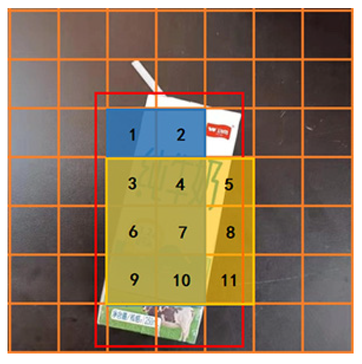
In order to make the model converge faster and make the final loss values as small as possible, assigning positive and negative prediction labels is a very important step. OTA (Optimal Transport Assignment) is a sample assignment strategy, which has four major elements: loss aware, center prior, dynamic top-k, and global view. To reduce the training time and simplify the process of fuzzy grid points using global information, YOLOX adopts SimOTA for the dynamic assignment of positive and negative samples. Firstly, the positive sample region proposal should be determined. Taking Figure 3 as an example, the red bounding box is the ground truth, the blue region A {1, 2, 3, 4, 6, 7, 9, 10} is the grids inside the ground truth, and the yellow region B {3, 4, 5, 6, 7, 8, 9, 10, 11} is all the grids within a grid distance extending outward from the center of the target. Then, the region C {3, 4, 6, 7, 9, 10}, the intersection of A and B, is consistent with both being in the ground truth and the center prior.
Secondly, the for each grid-generated prediction is calculated as:
where and are classification loss and regression loss, and the value of is 1 for grids that are not inside the region C and 0 otherwise.
Finally, the IoU (Intersection over Union) of each prediction and ground truth in region A is calculated. The topK algorithm is used to find the sum of the top 10 largest IoU values, and rounded down as the dynamic positive sample number . Again, we use the topK algorithm to find the grid points corresponding to the top smallest as positive samples. The rest are all negative samples. Due to the above-mentioned SimOTA for positive sample dynamic assignment, YOLOX achieves anchor free, thus reducing the preset parameters and improving the generalization ability of the model.
To achieve a better trade-off between the inference speed and accuracy, we choose YOLOX-m as the object detection model for optimization, which provides predicted results for visual sorting.
3.2.2. Data Augmentation
Data augmentation can make use of limited image samples to create more complex detection scenes. By increasing the training samples, the network overfitting is alleviated and the detection effect can be further improved.
Traditional data augmentation mainly includes optical transformation, geometric transformation, and adding noise. The three methods are combined as the traditional data augmentation strategy.
Mosaic [38] augmentation strategy randomly splices four images. Mixup [39] augmentation strategy performs a weighted combination of pixel points from two images:
where is the pasted image, is the original image, is the fused image, and the weight . The scale jitter coefficient is introduced to scale the pasted images before weighting. The standard scale jitter coefficient is 0.8~1.25, and the large-scale jitter coefficient is 0.1~2.0.
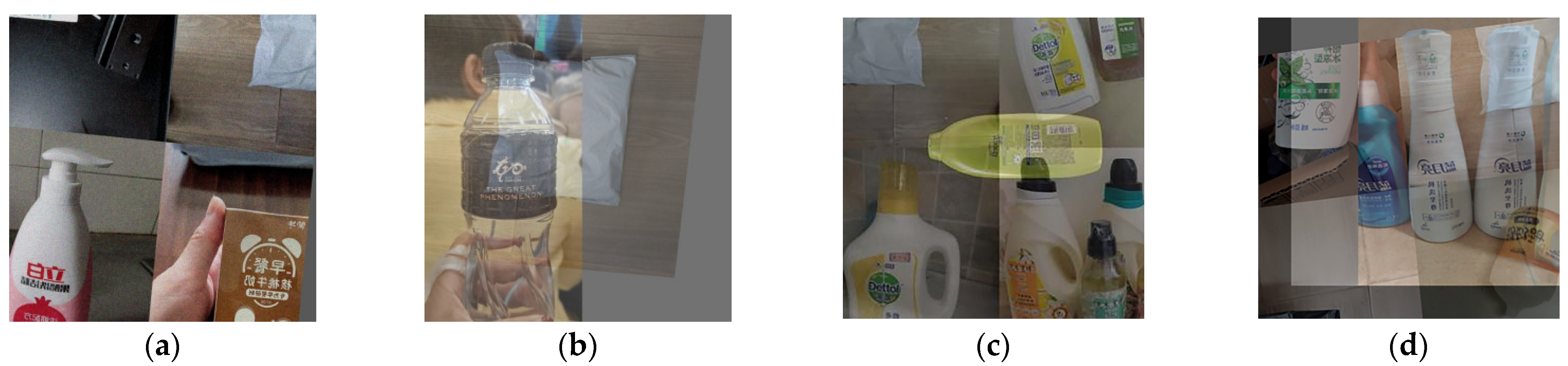
We use the aforementioned data augmentation in combination. To ensure randomness, the threshold is set to adjust the degree of augmentation of various strategies. The effects of different combined strategies are shown in Figure 4.
3.2.3. Deployment and Acceleration
Aiming at the problem of CNN with a large number of redundant parameters, this paper adopts two deployment acceleration methods, BN (Batch Normalization) layer fusion and mixed precision inference, to further improve the efficiency of the model.
BN layer fusion refers to merging the BN with the convolutional layer during model inference, so that the parameters pass through only the fused convolutional layer during the forward operation, thereby saving computational resources and accelerating model inference. The BN layer serves to normalize the data processed by the convolutional layer, which is beneficial to accelerate the convergence of the model and prevent overfitting. Therefore, the BN layer is placed after the convolution layer and before the activation layer. The three are combined as the basic module for massive stacking. Suppose the input is computed by the convolutional layer as follows:
where and are the parameters of the convolutional layer. After the BN layer, the following is obtained:
where is a small constant for computational stability, and are the mean and variance of training samples, and and are trainable parameters, which are regulated by gradient descent during training. In order to facilitate the analysis of the BN layer output, let:
Then is simplified as:
In the process of model inference, when , , , are determined, the convolutional layer parameters and can be modified according to the BN layer parameters, thus removing the separate BN layer and achieving fusion for the purpose of accelerated inference.
There are three floating point formats: half-precision (FP16), single-precision (FP32), and double-precision (FP64). Mixed precision inference is a precision accumulation method that uses both FP16 and FP32 during model inference. The model is trained and inferred with FP32 for computation and storage by default. The length occupied by FP16 is 16 bits, which is half of FP32. Adopting FP16 can reduce the parameter space occupied during the computation and improve the computational speed. However, the effective data representation range of FP16 is smaller than that of FP32. Using only FP16 has the problem of round-off error, that is, some data are forced to be rounded because of exceeding the representation range of FP16, resulting in a decline in model accuracy. Specifically, in the forward computation, the parameters are converted to FP16 for matrix multiplication and FP32 for matrix addition to make up for the loss of accuracy. In theory, mixed precision inference can speed up inference and save memory usage with negligible loss of precision.
3.3. Multiple Object Tracking
3.3.1. DeepSORT
For the input video sequence, information such as bounding box, confidence, and feature is output by the detector, which is filtered according to the confidence and input to the tracker for matching. The core of the DeepSORT algorithm lies in recursive Kalman filtering and frame-by-frame data association. Kalman filtering is an optimal estimation algorithm capable of generating a respective tracker for each object, which is used to estimate the position where each object will be located in the next frame. The Kalman filter predicts the trace of the object based on constant velocity motion and a linear observation model. It uses eight parameters to describe the state of the object at a certain time:
where represents the 2D pixel location of the bounding box’s center. and are the aspect ratio and height of the bounding box, respectively. The remaining variables represent the motion information of the object in the image coordinate system.
DeepSORT adopts a certain rule to match and associate the detection results with the tracking results. The Kalman filter uses the detection results of the previous frame to output the prediction boxes of all objects in the current frame, denoted as the set . The object detection model outputs the prediction boxes of all objects in the current frame, denoted as the set . The process of establishing the matching relationship for prediction boxes in and can be regarded as a bipartite graph problem, which can be efficiently solved using the Hungarian algorithm with minimal matching cost. In terms of data association, both the motion information and the appearance information of the object are considered to improve the matching effect of the Hungarian algorithm and reduce the number of identity switches.
The motion information is associated by using the Mahalanobis distance:
where and represent the bounding box detection and the track distribution, respectively. is the covariance matrix.
When motion uncertainty is high, using only the Mahalanobis distance is prone to association errors. Therefore, DeepSORT introduces appearance information for association, and measures the smallest cosine distance between the track and detection:
where denotes the appearance feature vector of the object, and denotes the feature vector in the corresponding feature set of the prediction box of the track.
When both the Mahalanobis and cosine distances meet their respective thresholds, is a hyperparameter, and the final metric is obtained by linear weighting:
In addition, DeepSORT introduces a matching cascade that gives priority to more frequently seen objects to ensure the continuity of tracking. The Kalman filter will update and output tracking results when the matching is successful, while the unmatched detection result and the unmatched tracking result will be matched by intersection over union.
3.3.2. Deep Cosine Metric Learning and Optimization
The cosine distance, also known as cosine similarity, is measured by calculating the cosine of the angle between two vectors. The higher the consistency of the pointing direction of two vectors, the higher the cosine similarity. When DeepSORT adopts cosine distance to associate appearance information, it uses CNN to extract features of tracking objects. The appearance feature set is established, and the relationship between the feature vectors is used to determine whether the detection results match the tracking results.
The feature extractor employed by DeepSORT is a wide residual network [40]. It is trained on a pedestrian dataset and suitable for the pedestrian tracking task. To solve the plastics tracking problem and to keep the running cost as low as possible while ensuring tracking accuracy, ShuffleNetV2 [41] is used as the feature extractor in this paper. The network is trained offline on the plastics dataset so that it can better extract plastic features and thus optimize the cosine metric of the tracker.
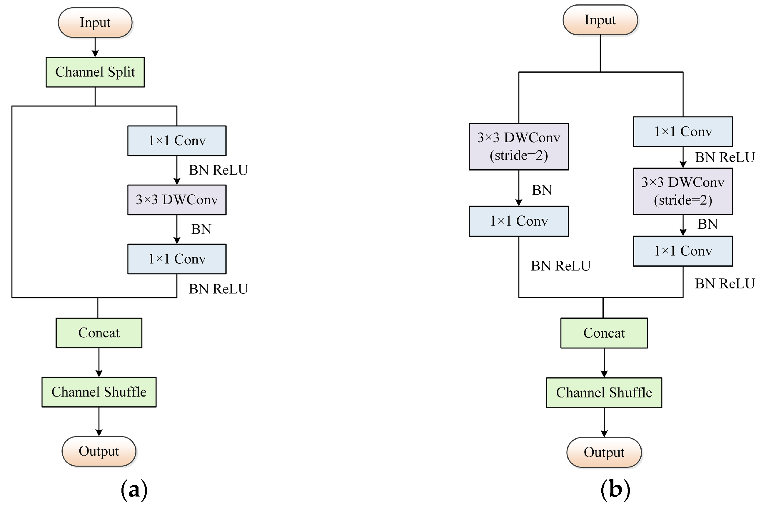
ShuffleNetV2 is a lightweight CNN with strong performance and applicability. The building blocks of this model are shown in Figure 5. Figure 5a shows the basic unit; the input of the feature channel is split into two branches by channel split. One branch is mapped equally, and the other branch performs two 1 × 1 convolutions and one 3 × 3 depthwise convolution. The two branches are concatenated after completing their respective operations, and then the channel shuffle operation is carried out. In this case, the number of input and output channels is the same, which can effectively reduce the memory access consumption time. The purpose of channel shuffle is to ensure feature information communication between different branches and improve the generalization of the model. Figure 5b shows the downsampling unit. All features are input into two branches, and a series of convolution operations are performed respectively. Features are output after concatenation and channel shuffle.
The architecture of ShuffleNetV2 is a stack of the previously mentioned building blocks, since this paper does not perform classification but uses the network for object appearance feature extraction in the tracking task. Therefore, the output of the global pool is used as the feature mapping for the final output.
3.3.3. Metrics and Optimization of Matching
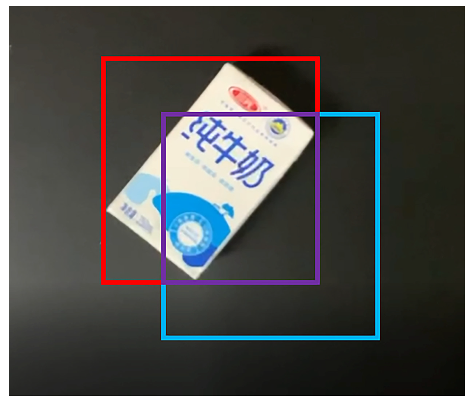
In the tracking task, [42] is used to measure the matching degree between the detection box and the prediction box. In the matching stage of DeepSORT, is applied to process the unmatched detection results and tracking results, and the cost matrix is computed. The Hungarian algorithm uses this matrix to further solve the assignment problem. Finally, the object trace is formed.
is the ratio of intersection to union, and the equation is as follows:
As shown in Figure 6, the red box and the blue box represent the detection box and the prediction box, respectively. The purple box is the overlap area of and .
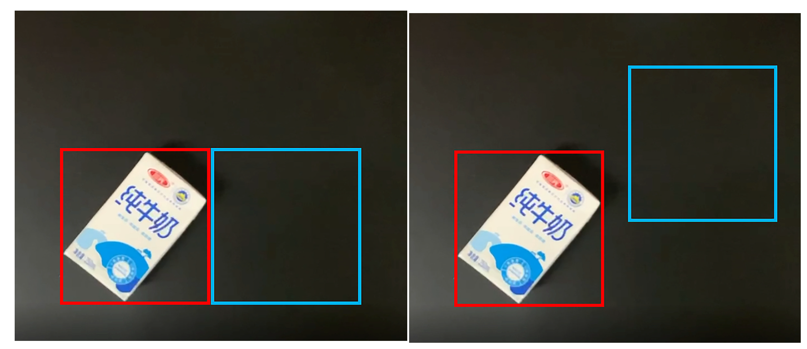
However, there are the following problems when using to measure the degree of overlap between the detection box and the prediction box:
- 1.
- When there is no intersection between the detection box and the prediction box, the relative distance between the two cannot be reflected at this time. This case is shown in Figure 7.
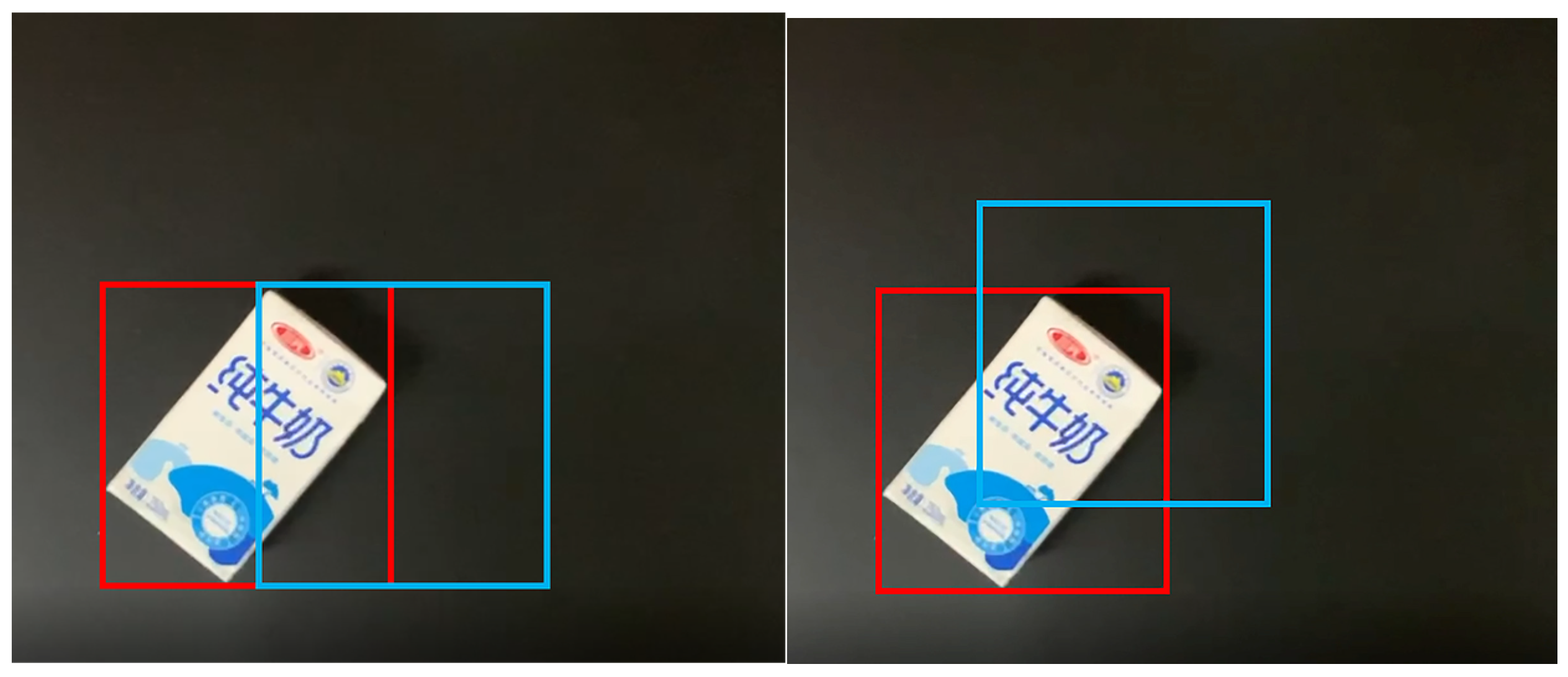
- 2.
- When the intersection of the detection box and the prediction box exists and is equal, it is impossible to distinguish the matching effect in different overlapping states using . This case is shown in Figure 8.
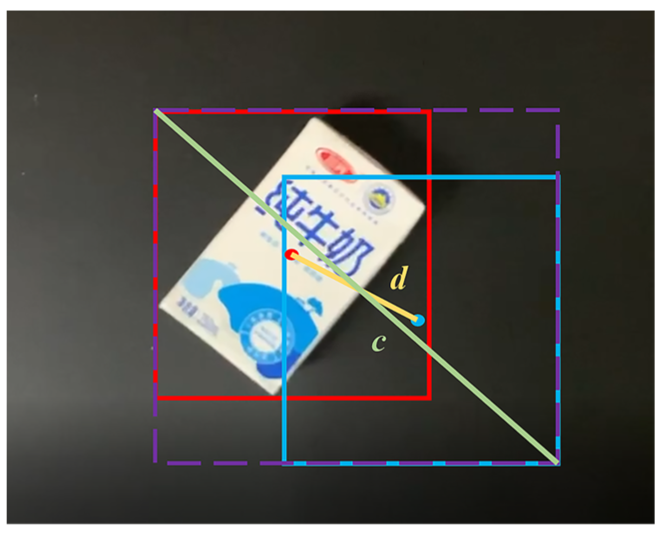
In order to solve the above problems, this paper adopts (Distance Intersection over Union) [43] instead of in DeepSORT, and its equation is as follows:
where and denote the center points of and , respectively. The purple dotted box represents the minimum bounding rectangle covering the two boxes, and the diagonal length labeled . is the Euclidean distance labeled , as shown in Figure 9.
For the detection box and prediction box, considers three important factors at the same time: the overlap area, the non-overlap area and the central point distance. It can describe the matching relationship more comprehensively.
3.4. Workflow of Plastic Dynamic Detection
3.4.1. Information Acquisition Logic Based on Virtual Two-Line Detection
The location, class, and ID (identity) of the plastic can be obtained using the optimized YOLOX and DeepSORT. However, simply obtaining this information is not sufficient for plastic sorting. It is crucial to accurately and methodically acquire information about each plastic and send it to the robotic arm.
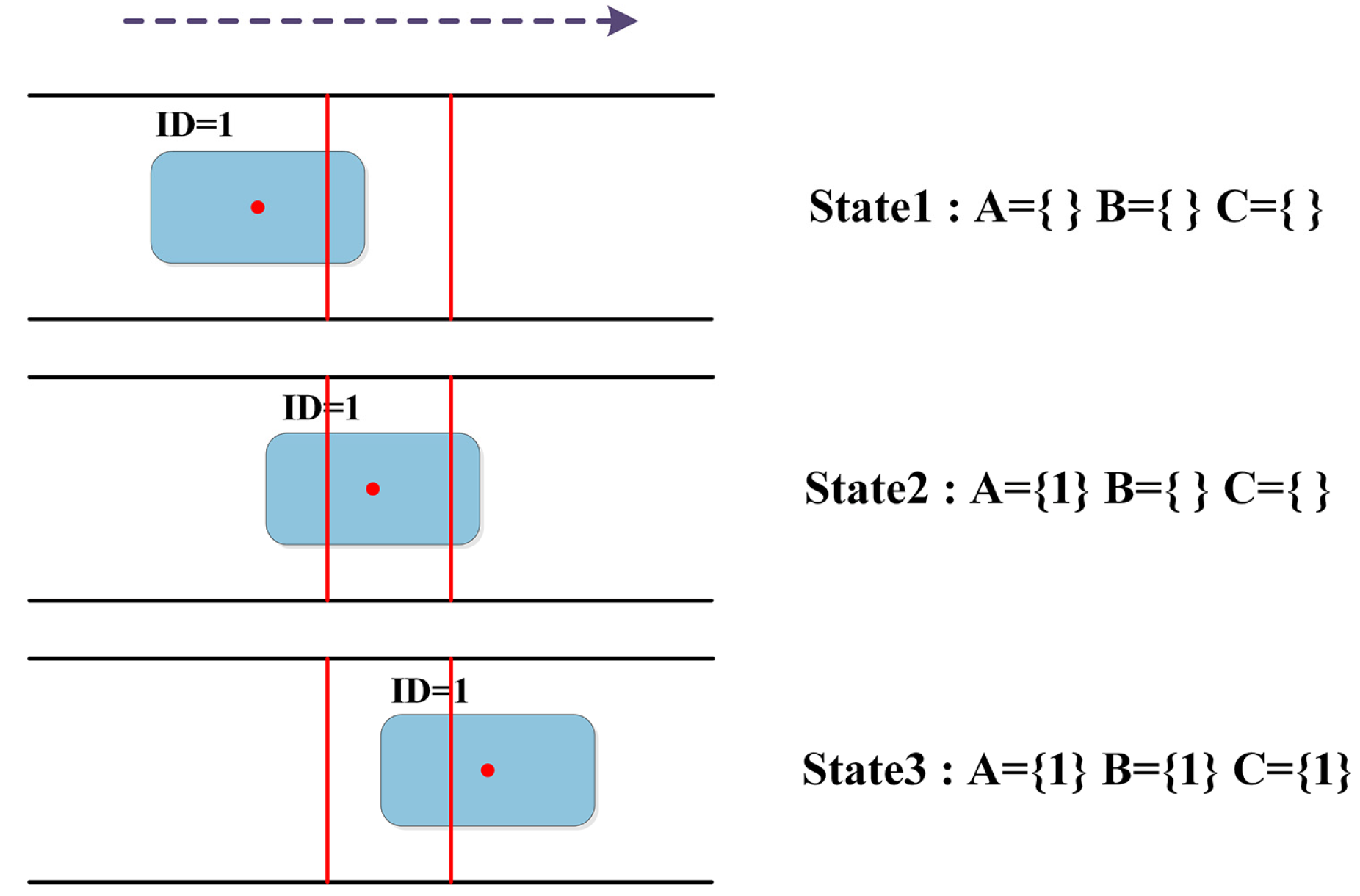
We set up two virtual detection lines called the object entry line and the object exit line. They constitute the plastic detection area. The system no longer acquires and records information about the plastics outside the detection area. To filter out missed detections and false detections that take too long, the plastic is determined as the sorting object only if it meets the criteria of being continuously tracked and passing through the object entry line and the object exit line in sequence. In this paper, the state of the plastic is judged based on the relative position between the center point of the bounding box and the two virtual lines. As shown in Figure 10, the red dot represents the center point and the red lines represent the detection lines. We set the sets A, B, and C. A records the IDs of all plastics that pass through the object entry line. B records the IDs of all plastics that pass through the object exit line. C records the IDs that exist in both A and B, which are the sorting objects after preliminary filtering.
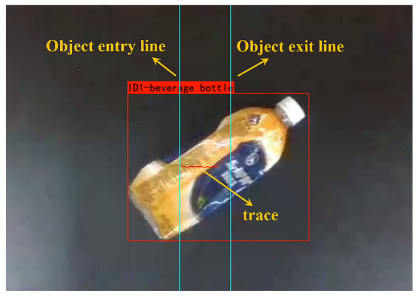
As shown in Figure 11, in this paper, the class output by YOLOX and the ID assigned by DeepSORT are added to the bounding box. Plastics with the same ID in each frame are considered as the same object. The relative motion trace of the plastics is obtained by connecting the center points of adjacent frames. The algorithm only records the trace of the plastic in the detection area.
When the plastic is determined as the sorting object, its angle, height, and velocity are calculated. To obtain more accurate information, the distance between the two virtual detection lines is set as small as possible, and the object exit line is set directly below the camera as far as possible. In this paper, a queue is maintained to record and send information about the plastics to be sorted. The queue adopts the first in, first out principle, and the information is added sequentially to the end of the queue in the form of a list. The plastic information is represented as:
where is the center point of the plastic. , , , denote the class, angle, height, and velocity of the plastic, respectively. is the timestamp when the plastic first crosses the object exit line.
Due to the heavy workload of plastic sorting, it is necessary to minimize the single sorting distance, so a virtual grasping baseline is set to limit the movement of the robotic arm. When the center point of the plastic reaches the grasping baseline, the robotic arm picks it and places it in the specified position. The workflow of plastic sorting is shown in Figure 12.
3.4.2. Calculation of Plastic Angle
The plastic is at a random angle on the conveyor belt. If the angle of the end effector is constant, it may grasp other adjacent plastics. In addition, adjusting the angle can maximize its fitting area with the plastic and improve the accuracy of grasping. Therefore, it is necessary to measure the angle of each plastic, and the robotic arm makes adjustments based on the angle information.
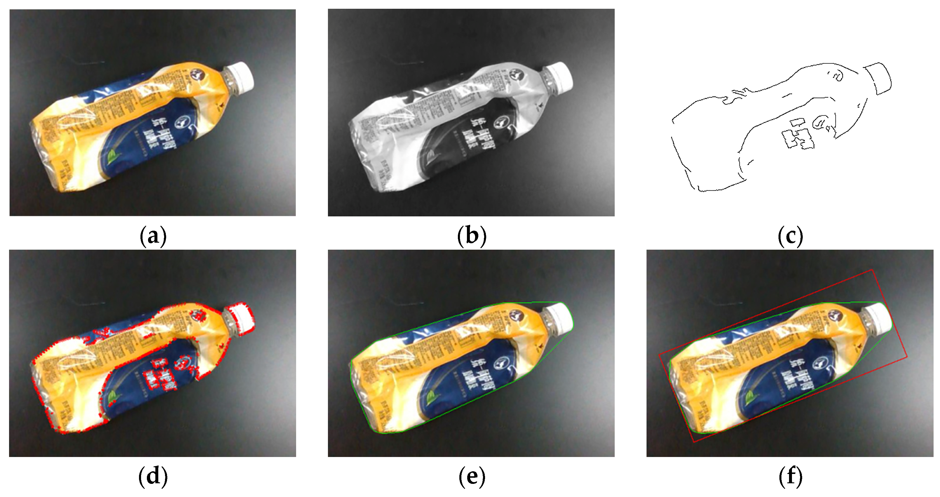
The key to calculating the angle is solving for the OBB (Oriented Bounding Box), also known as the minimum bounding rectangle. To reduce irrelevant information, the image is first cropped and gray scale processing is performed. Then, the Canny [44] edge extraction operator combined with Gaussian smoothing noise reduction is applied to realize the edge detection.
The minimum bounding rectangle is solved in three steps. First, the contour points are extracted. Then, Graham’s scan method [45] is used to solve the convex hull. Finally, the minimum bounding rectangle is solved according to the idea of rotating calipers. The process of solving the angle is shown in Figure 13.
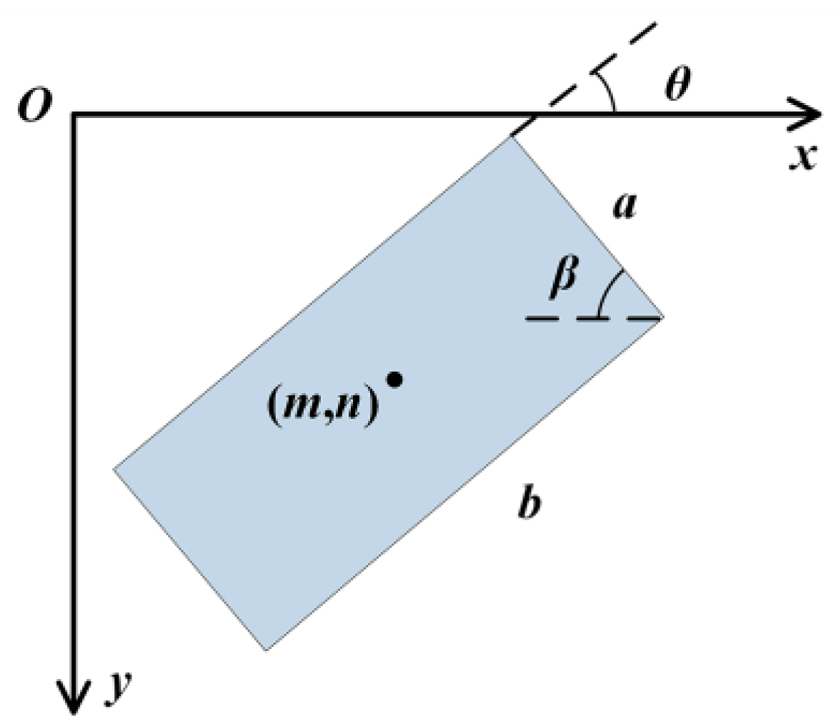
The end effector posture adjustment takes a long time when the angle change is too large. To avoid this problem, we constrain the angle output range to be [0°,90°]. The corresponding output rule is shown in Figure 14.
The output result is specified as , where is the center point of the minimum bounding rectangle, and are the length and width of the rectangle, β is the angle between the side of length and the -axis, and is the angle between the side of length and the -axis, which is the angle of the plastic. Taking counterclockwise as the positive angle, the angle is calculated as follows:
3.4.3. Calculation of Plastic Height
The height of waste plastics varies, so each plastic should be measured, as inaccurate height measurement will directly lead to the failure of the robotic arm to grasp.
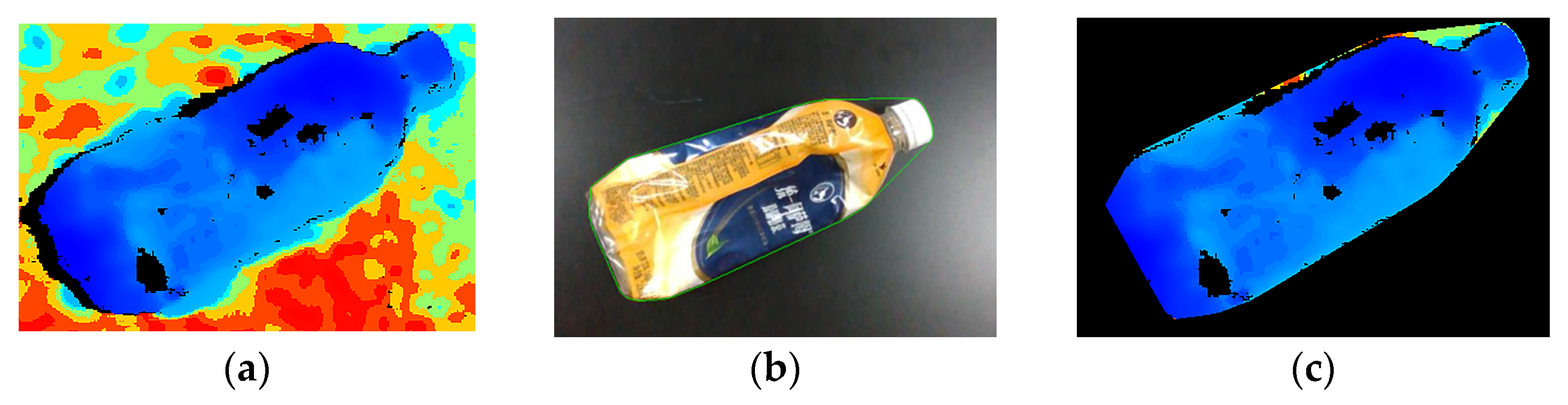
As shown in Figure 15, the image mask technique is first employed to extract the region of interest, and the convex hull obtained during angle calculation is filled as the plastic region mask. All values of the region where the plastic is located in the depth map are extracted using the bitwise and operation of the image while assigning the other regions to 0.
Assume that the installation height of the camera relative to the conveyor belt is meters. The plastic height calculation process is as follows:
- 1.
- To obtain the height information of the non-black region in Figure 15c, only non-zero values are selected. Tile them as a one-dimensional list of length .
- 2.
- The topK algorithm is adopted to obtain the first small values.
- 3.
- To reduce the interference of the plastic surface bulge or the camera measurement error, the topK algorithm is again used to remove the first values in the obtained values of (2). The distance set U can be obtained.
- 4.
- The height of the object is minus the mean of all data in the set U. The equation is as follows:where , is 5, and is 40. Theoretically, the height is obtained from the 7/40 top area of the object. For plastic with an uneven surface, the integrated vacuum sucker can successfully grasp it by sucking only a small part of the top area.
3.4.4. Calculation of Plastic Velocity
The configuration between the camera and the robotic arm in this paper is eye-to-hand. After the plastic leaves the camera’s field of view, it still needs to be transferred a certain distance to reach the grasping baseline. Therefore, it is necessary to calculate the relative motion velocity of the plastic to ensure accurate grasping. In this paper, the velocity is solved with the help of the displacement of the plastic between the two aforementioned virtual detection lines. Assuming that the transmission direction and vertical direction of the conveyor belt are the x-axis and y-axis, respectively, theoretically, the plastic will not be displaced along the y-axis. During the time to , we save the data in the format . Since we only consider a small distance directly below the camera, the velocity can be solved based on the first and last points:
When the measurement error is large, the error will be further amplified after some time, leading to the failure of the grasp. The data measurement noise of our system mainly comes from the prediction error of object detection. We adopt Kalman filtering to filter the measured velocity. It outputs a more reasonable predicted value based on the system variables, and this value is used as the final relative motion velocity of the plastic.
4. Experimental Results and Discussion
4.1. Experimental Configuration
4.1.1. Evaluation Indicators
In this paper, we focus on the quantitative evaluation of the performance of plastic detection and tracking algorithms. For the accuracy of the plastic detection model, the widely used mAP (mean Average Precision) is adopted as the evaluation index. The IoU threshold is related to the localization accuracy and corresponds to different mAPs. The IoU threshold is set to 10 values with 0.05 intervals from 0.5 to 0.95. When the threshold is , the evaluation index is , and the equation is as follows:
The inference speed of the model is affected by many factors such as model size, hardware characteristics, memory access time, cost, and so on. To obtain the inference speed, we measured the time it takes for the model to compute an image several times under the specified hardware conditions.
For plastic tracking with the practical application scenario it should be ensured that the plastic can be tracked accurately and continuously, and the switch should be reduced as much as possible. Therefore, the following three indicators are selected to focus on evaluating the performance of the tracker.
is the total number of missed targets. is the number of target identity switches. is a comprehensive indicator to measure the performance of the tracker and is calculated as follows:
where is the total number of false positives and is the total number of ground truth.
4.1.2. Experimental Environment
The software environment for offline training in this experiment is the Ubuntu18.04 operating system, the Python3.7 development language, and the PyTorch deep learning framework. The hardware environment is the Intel i9-10980XE CPU, 32 G memory, and the Nvidia GeForce RTX3090 graphics card. The algorithm is run online on the Win 10 operating system, and the rest of the software environment is the same as the offline training. The hardware environment is the Intel i7-10700 CPU, 16 G memory, and the Nvidia GeForce RTX 3060Ti graphics card.
4.2. Experiments of Plastic Detection
4.2.1. Influence of Data Augmentation on Performance
To verify the effectiveness of data augmentation, we conducted ablation experiments to test the effect of various strategies to improve the detection accuracy of YOLOX-m.
Since the images generated using mosaic or mixup augmentation have large differences from the true distribution, inaccurate annotation boxes will be generated. Therefore, to allow the model to converge with naturally distributed data, each experiment was trained for 100 epochs. We closed the relevant data augmentation for the last 40 epochs while using L1 loss to alleviate overfitting. The experimental results are shown in Table 2.
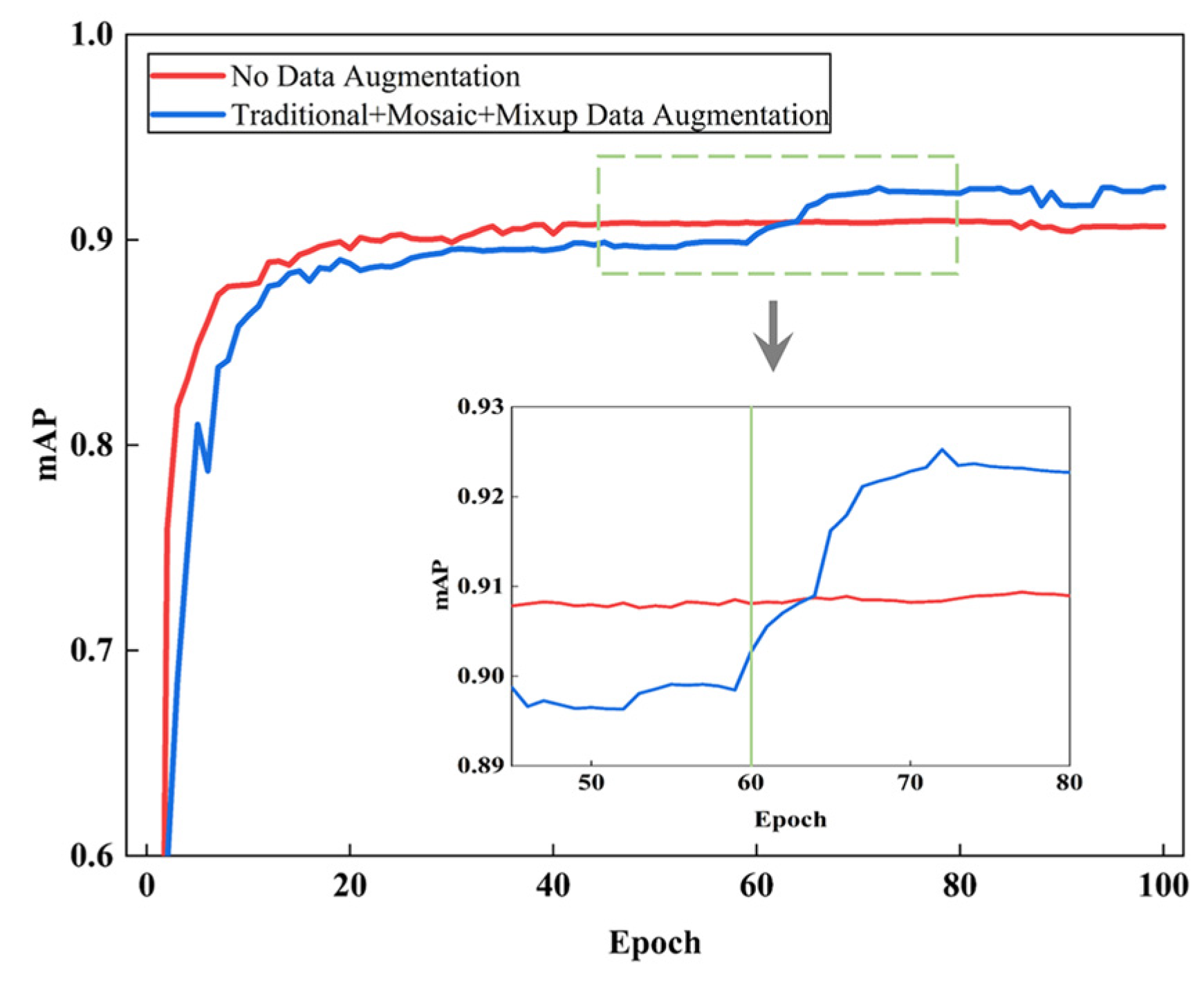
Figure 16 shows the effect of model training. The accuracy grows fast at first when data augmentation is not used, but the mAP increases insignificantly or even decreases with increasing iterations. When the three augmentation strategies are combined, the mAP is lower in the early stage because mosaic and mixup increase the training difficulty. When these two data augmentations are closed, mAP grows again and achieves better training results.
When using the best data augmentation strategy, the mAPs for each category are shown in Table 3.
4.2.2. Influence of Deployment Acceleration on Performance
This experiment focuses on testing the model inference time. In order to truly reflect the actual operation of the model, the test conditions are the same as the hardware configuration of the system running online. The same 100 test images were used for each experiment, and the test was repeated 10 times based on the YOLOX with the best data augmentation effect to compute the average inference time for each image. The results are shown in Table 4.
Adopting BN layer fusion and mixed precision inference, the model accuracy is almost unchanged, and the improvement in inference speed is 2% and 2.28%, respectively. Using both methods simultaneously, the inference time is further reduced to 16.811 ms. When the model is run, the video memory usage is reduced from 1.5 GB to 0.7 GB.
4.3. Experiments of Plastic Tracking
4.3.1. Training of Feature Extraction Network
The feature extraction network of the original DeepSORT is trained on the pedestrian dataset, specifically for pedestrian tracking, and has not learned the features of plastics. To solve the problem of multiple object plastic tracking, the feature extraction network needs to be retrained so as to optimize the metric of cosine distance and the construction of a related matrix.
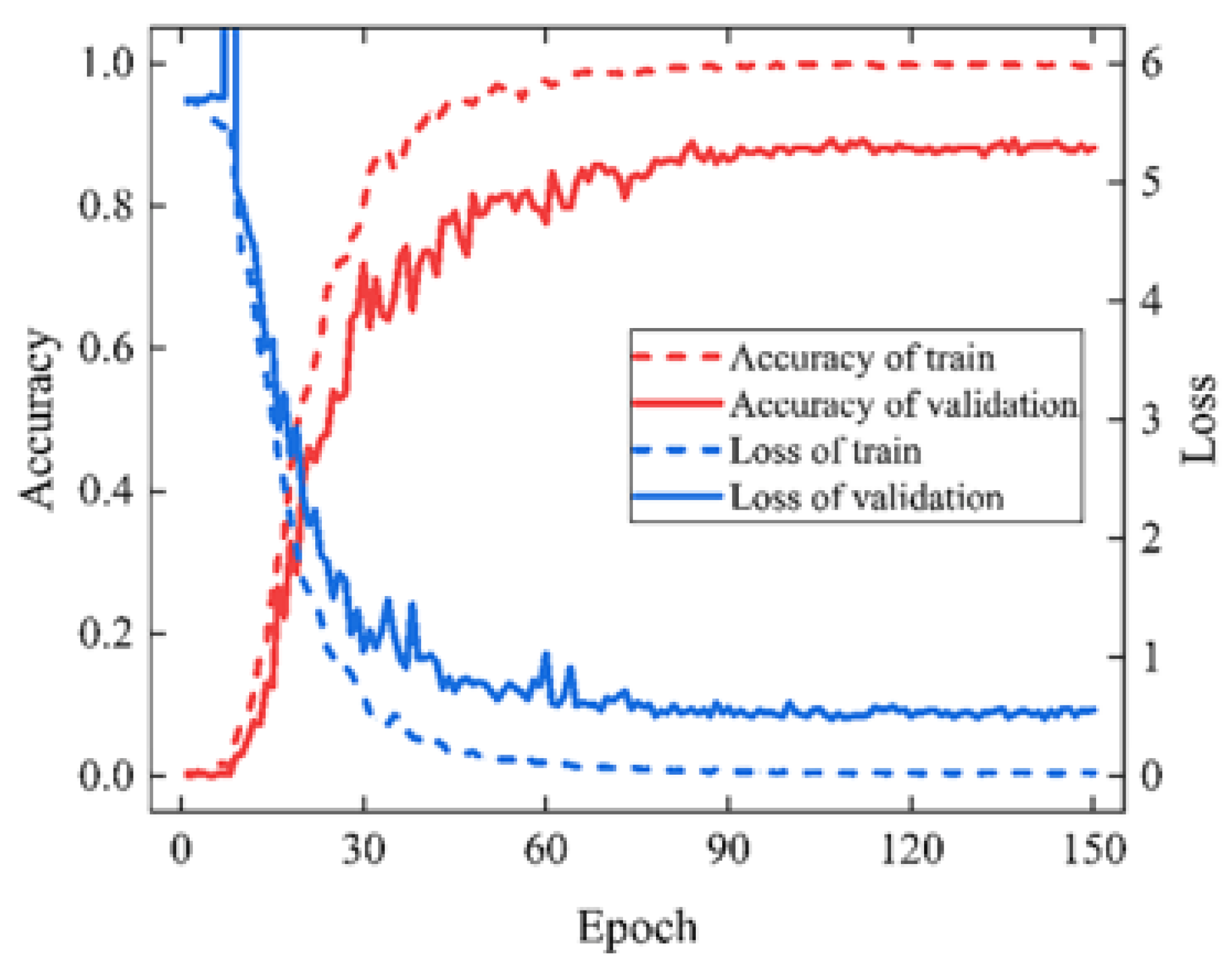
The learning rate of the original algorithm is decaying at equal intervals, but for the dataset in this paper, the convergence effect is not good enough when using this strategy. We therefore used a combination of warm up and cosine annealing to adjust the learning rate [46], with an initial learning rate of 0.1 and a step size of 5. We adopted stochastic gradient descent (SGD) and cross entropy loss function for training, and we set the batch size to 64. We trained the model for a total of 150 epochs. Figure 17 shows the training process of ShuffleNet on the plastic tracking dataset; the validation accuracy reaches 88.15%. The improved model has only 1.61 MB parameters, which is approximately 1/7 of the original model and is more accurate.
4.3.2. The Improvement of DeepSORT
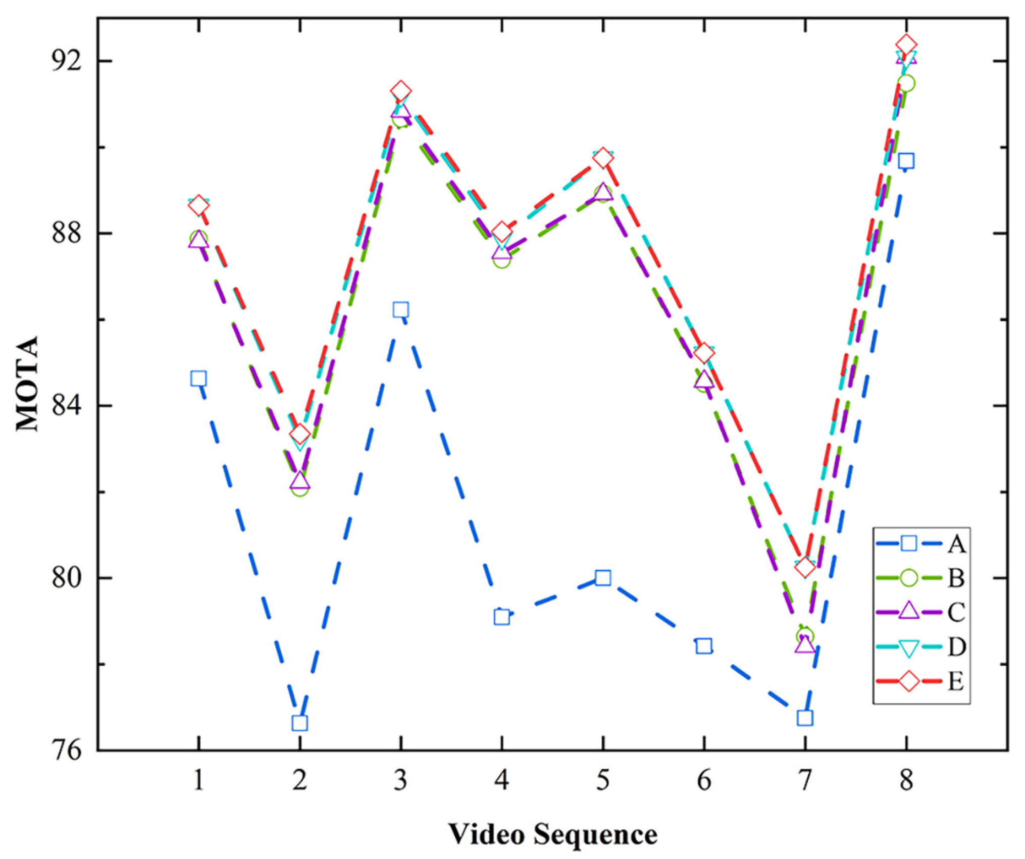
To further verify the effectiveness of improved strategies for the plastic tracking algorithm, we collected eight video sequences, which showed different arrangements of plastics on the conveyor belt. We constructed the dataset in MOT format for the ablation experiments. The results are shown in Table 5 and Figure 18.
In the base model, the original YOLOX is used to replace the detector of DeepSORT. From the results, it can be seen that each improvement strategy has different degrees of optimization effect on the base model. The best tracking result is achieved when the improved YOLOX detector, the ShuffleNet feature extraction network, and the DIOU metric are used simultaneously. At this point, MOTA achieves 87.45%, surpassing the algorithm before improvement by 6.39%. The improved DeepSORT with this strategy will be used for plastic tracking.
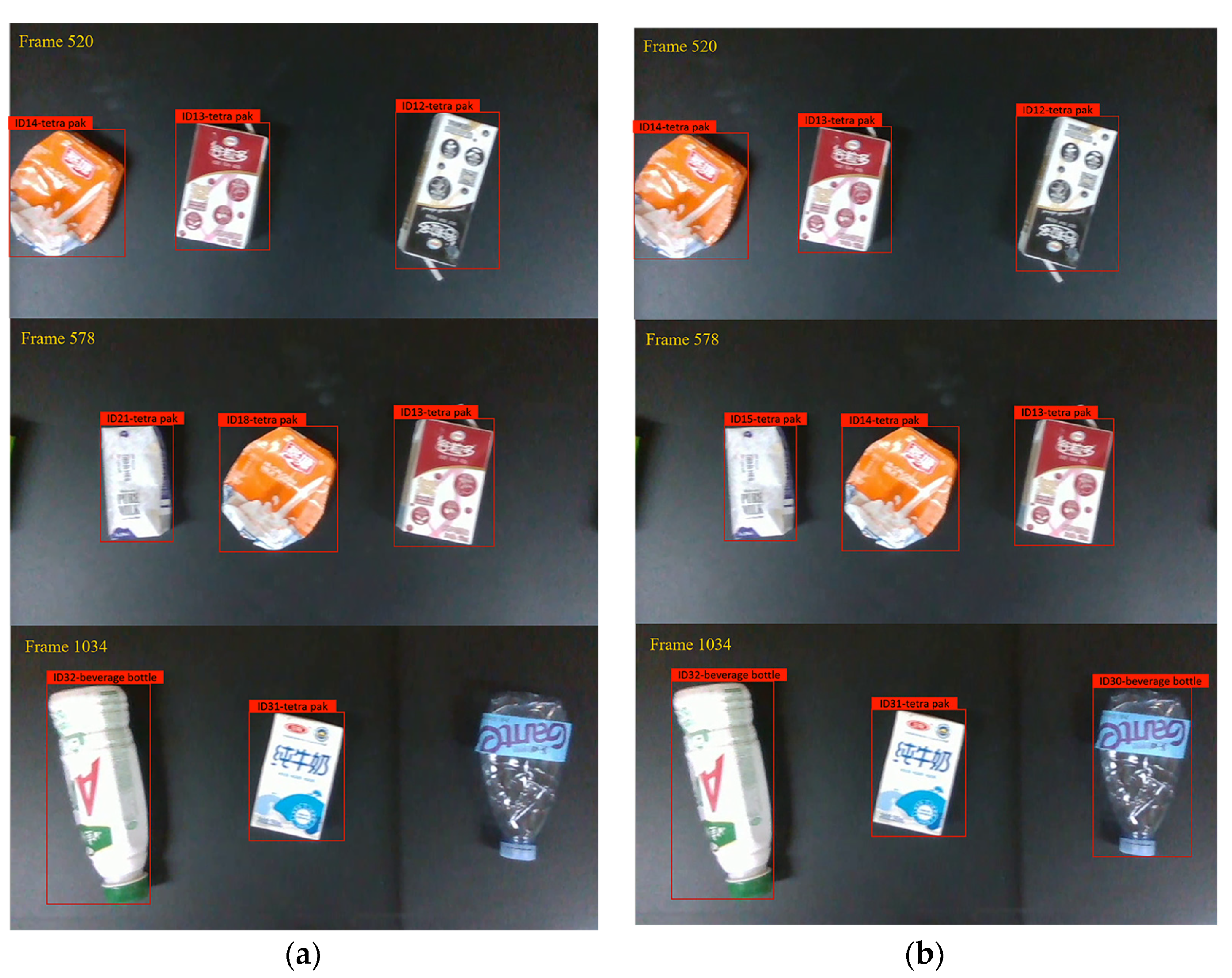
As shown in Figure 19, there are ID switches and a missing detection before the improvement. At this time, the plastic will not be determined as the sorting object, and the algorithm does not meet the requirements of this system to accurately detect and keep the ID unchanged. The tracking effect of the improved algorithm is more stable.
4.4. Performance Test of Waste Plastics Sorting System
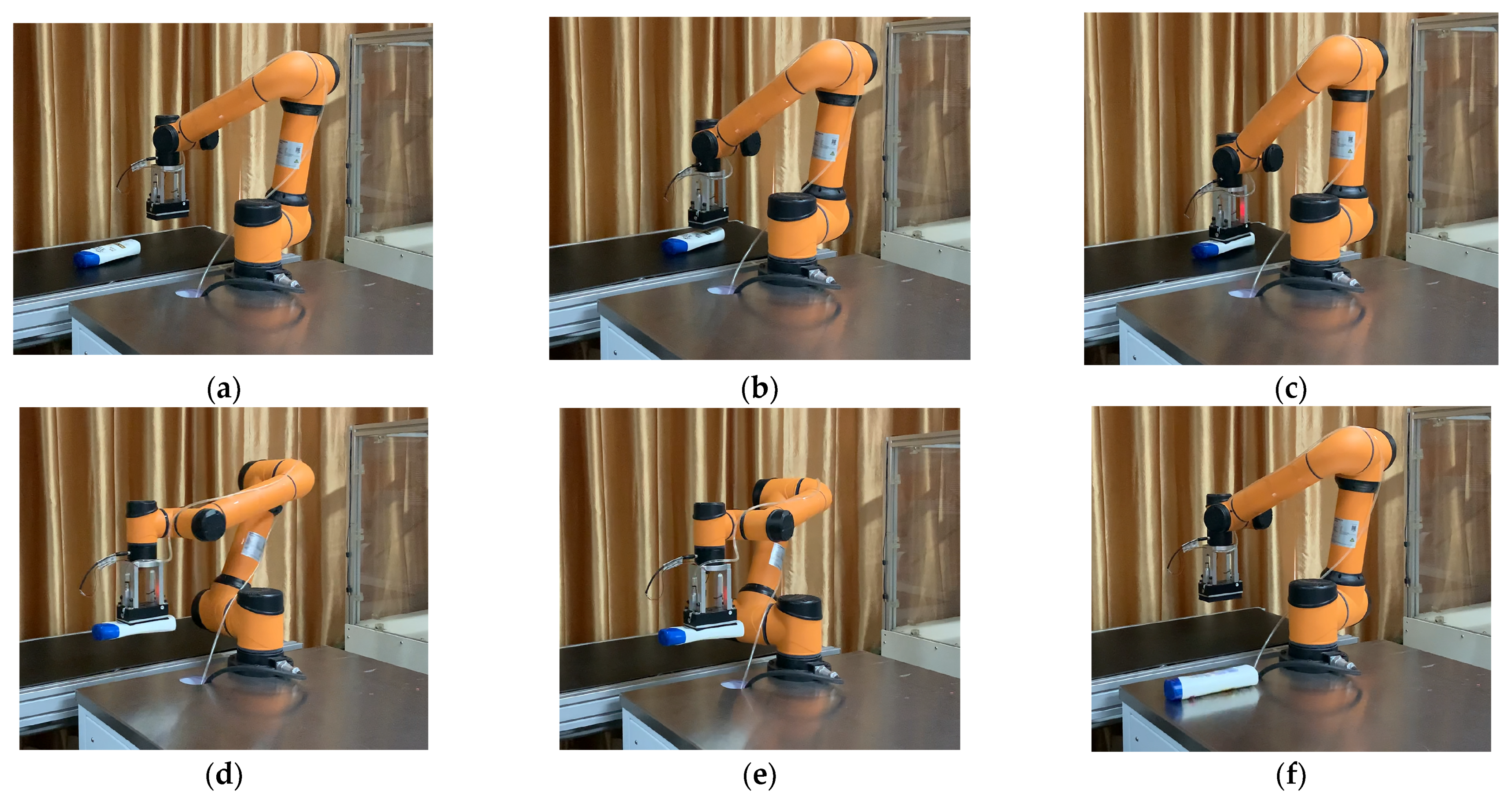
To test the sorting effect of this system, we put 50 plastics containing five categories at reasonable spacing on a conveyor belt, and the running speed of the conveyor belt was approximately 0.12 m/s. Figure 20 shows the stages in the process of sorting plastic by the robotic arm, and Table 6 shows the experimental results.
The method proposed in this paper can effectively detect plastics. Due to the limitation of the sorting device, the grasping effect is not good enough for plastic with uneven surfaces and smooth or light, soft material. Therefore, in subsequent work, the system performance can be further improved by adopting the more appropriate sorting device.
5. Conclusions
In order to improve the accuracy and efficiency of waste plastics sorting, this paper proposes a vision detection method based on deep learning to realize the real-time detection, tracking, and grasping of plastics on the conveyor belt. For the object detection model, multiple data augmentation combinations are adopted to improve accuracy. Two efficient deployment acceleration methods, BN layer fusion and mixed precision inference, are applied to improve efficiency. For the multiple object tracking algorithm, the feature extraction network and the matching metric are optimized to improve the tracking performance. Based on this, the two algorithms are combined to form a vision detection method more suitable for plastics. The information is filtered and extracted by the virtual detection line to determine the sorted objects. The experimental results show that the proposed method has good performance for dynamic plastic sorting. In addition, the waste plastics sorting system built in this paper uses the camera as a powerful sensor. The system no longer relies on other external sensors, avoiding installation and cost problems. It can be used for the real-time sorting of other complex objects with only minor adjustments, so it has certain versatility and application value.
Author Contributions
Conceptualization, S.W.; methodology, Y.Y.; software, Y.Y. and J.C.; validation, Y.Y.; investigation, S.W., Y.Y. and J.C.; resources, S.W.; data curation, S.W., Y.Y. and J.C.; writing—original draft preparation, Y.Y.; writing—review and editing, Y.Y. and S.W.; visualization, Y.Y.; supervision, S.W.; project administration, S.W.; funding acquisition, S.W. All authors have read and agreed to the published version of the manuscript.
Funding
This research was funded by the National Key Research and Development Project from the Ministry of Science and Technology (grant number 2019YFC1908201), the Key Program of the National Natural Science Foundation of China (grant number 51933004), and the Introduced Innovative Scientific Research Team of Dong Guan City (grant number 2020607105006).
Institutional Review Board Statement
Not applicable.
Informed Consent Statement
Not applicable.
Data Availability Statement
Not applicable.
Conflicts of Interest
The authors declare no conflict of interest.
References
- Huang, S.; Wang, H.; Ahmad, W.; Ahmad, A.; Ivanovich Vatin, N.; Mohamed, A.M.; Deifalla, A.F.; Mehmood, I. Plastic Waste Management Strategies and Their Environmental Aspects: A Scientometric Analysis and Comprehensive Review. Int. J. Environ. Res. Public Health 2022, 19, 4556. [Google Scholar] [CrossRef] [PubMed]
- OECD. Global Plastics Outlook; OECD: Paris, France, 2022. [Google Scholar]
- Fu, S.C.; Fang, Y.; Yuan, H.X.; Tan, W.J.; Dong, Y.W. Effect of the medium’s density on the hydrocyclonic separation of waste plastics with different densities. Waste Manag. 2017, 67, 27–31. [Google Scholar] [CrossRef] [PubMed]
- Pita, F.; Castilho, A. Separation of plastics by froth flotation. The role of size, shape and density of the particles. Waste Manag. 2017, 60, 91–99. [Google Scholar] [CrossRef]
- Felsing, S.; Kochleus, C.; Buchinger, S.; Brennholt, N.; Stock, F.; Reifferscheid, G. A new approach in separating microplastics from environmental samples based on their electrostatic behavior. Environ. Pollut. 2018, 234, 20–28. [Google Scholar] [CrossRef]
- Shuliang, Z.; Yiqiang, L.; Dewen, T. Analysis of horizontal air-separator field of municipal solid waste based on CFD. Adv. Mater. Res. 2014, 1030–1032, 1155–1162. [Google Scholar] [CrossRef]
- Wu, X.Y.; Li, J.; Yao, L.P.; Xu, Z.M. Auto-sorting commonly recovered plastics from waste household appliances and electronics using near-infrared spectroscopy. J. Clean. Prod. 2020, 246, 118732. [Google Scholar] [CrossRef]
- Yang, J.C.; Wang, C.G.; Jiang, B.; Song, H.B.; Meng, Q.G. Visual Perception Enabled Industry Intelligence: State of the Art, Challenges and Prospects. IEEE Trans. Ind. Inform. 2021, 17, 2204–2219. [Google Scholar] [CrossRef]
- Javaid, M.; Haleem, A.; Singh, R.P.; Rab, S.; Suman, R. Exploring impact and features of machine vision for progressive industry 4.0 culture. Sens. Int. 2022, 3, 100132. [Google Scholar] [CrossRef]
- Xia, W.J.; Jiang, Y.P.; Chen, X.H.; Zhao, R. Application of machine learning algorithms in municipal solid waste management: A mini review. Waste Manag. Res. 2022, 40, 609–624. [Google Scholar] [CrossRef]
- Torres-García, A.; Rodea-Aragón, O.; Longoria-Gandara, O.; Sánchez-García, F.; González-Jiménez, L.E. Intelligent Waste Separator. Comput. Y Sist. 2015, 19, 487–500. [Google Scholar] [CrossRef]
- Özkan, K.; Ergin, S.; Işık, Ş.; Işıklı, İ. A new classification scheme of plastic wastes based upon recycling labels. Waste Manag. 2015, 35, 29–35. [Google Scholar] [CrossRef] [PubMed]
- Paulraj, S.G.; Hait, S.; Thakur, A. Automated municipal solid waste sorting for recycling using a mobile manipulator. In Proceedings of the ASME 2016 International Design Engineering Technical Conferences and Computers and Information in Engineering Conference, IDETC/CIE 2016, Charlotte, NC, USA, 21–24 August 2016. [Google Scholar]
- Wang, Z.; Peng, B.; Huang, Y.; Sun, G. Classification for plastic bottles recycling based on image recognition. Waste Manag. 2019, 88, 170–181. [Google Scholar] [CrossRef] [PubMed]
- Tan, Z.; Fei, Z.; Zhao, B.; Yang, J.; Xu, X.; Wang, Z. Identification for Recycling Polyethylene Terephthalate (PET) Plastic Bottles by Polarization Vision. IEEE Access 2021, 9, 27510–27517. [Google Scholar] [CrossRef]
- Lin, K.; Zhao, Y.; Kuo, J.-H.; Deng, H.; Cui, F.; Zhang, Z.; Zhang, M.; Zhao, C.; Gao, X.; Zhou, T.; et al. Toward smarter management and recovery of municipal solid waste: A critical review on deep learning approaches. J. Clean. Prod. 2022, 346, 130943. [Google Scholar] [CrossRef]
- Tamin, O.; Moung, E.G.; Dargham, J.A.; Yahya, F.; Omatu, S.; Angeline, L. Machine Learning for Plastic Waste Detection: State-of-the-art, Challenges, and Solutions. In Proceedings of the 2022 International Conference on Communications, Information, Electronic and Energy Systems (CIEES), Veliko Tarnovo, Bulgaria, 24–26 November 2022; pp. 1–6. [Google Scholar]
- Srinilta, C.; Kanharattanachai, S. Municipal Solid Waste Segregation with CNN. In Proceedings of the 2019 5th International Conference on Engineering, Applied Sciences and Technology (ICEAST), Luang Prabang, Laos, 2–5 July 2019. [Google Scholar]
- Zhang, Q.; Zhang, X.; Mu, X.; Wang, Z.; Tian, R.; Wang, X.; Liu, X. Recyclable waste image recognition based on deep learning. Resour. Conserv. Recycl. 2021, 171, 105636. [Google Scholar] [CrossRef]
- Wu, T.-W.; Zhang, H.; Peng, W.; Lü, F.; He, P.-J. Applications of convolutional neural networks for intelligent waste identification and recycling: A review. Resour. Conserv. Recycl. 2023, 190, 106813. [Google Scholar] [CrossRef]
- Zhao, Z.-Q.; Zheng, P.; Xu, S.-T.; Wu, X. Object Detection With Deep Learning: A Review. IEEE Trans. Neural Netw. Learn. Syst. 2019, 30, 3212–3232. [Google Scholar] [CrossRef] [Green Version]
- Guo, Z.; Wang, C.; Yang, G.; Huang, Z.; Li, G. MSFT-YOLO: Improved YOLOv5 Based on Transformer for Detecting Defects of Steel Surface. Sensors 2022, 22, 3467. [Google Scholar] [CrossRef]
- Zhao, J.; Zhang, X.; Yan, J.; Qiu, X.; Yao, X.; Tian, Y.; Zhu, Y.; Cao, W. A Wheat Spike Detection Method in UAV Images Based on Improved YOLOv5. Remote Sens. 2021, 13, 3095. [Google Scholar] [CrossRef]
- Wu, P.; Li, H.; Zeng, N.; Li, F. FMD-Yolo: An efficient face mask detection method for COVID-19 prevention and control in public. Image Vis. Comput. 2022, 117, 104341. [Google Scholar] [CrossRef]
- Arnold, E.; Dianati, M.; De Temple, R.; Fallah, S. Cooperative Perception for 3D Object Detection in Driving Scenarios Using Infrastructure Sensors. IEEE Trans. Intell. Transp. Syst. 2022, 23, 1852–1864. [Google Scholar] [CrossRef]
- Ye, A.; Pang, B.; Jin, Y.; Cui, J. A YOLO-based Neural Network with VAE for Intelligent Garbage Detection and Classification. In Proceedings of the 2020 3rd International Conference on Algorithms, Computing and Artificial Intelligence, Sanya China, 24–26 December 2020. [Google Scholar]
- Melinte, D.O.; Travediu, A.-M.; Dumitriu, D.N. Deep Convolutional Neural Networks Object Detector for Real-Time Waste Identification. Appl. Sci. 2020, 10, 7301. [Google Scholar] [CrossRef]
- Zhang, Q.; Yang, Q.F.; Zhang, X.J.; Wei, W.; Bao, Q.; Su, J.Q.; Liu, X.Y. A multi-label waste detection model based on transfer learning. Resour. Conserv. Recycl. 2022, 181, 106235. [Google Scholar] [CrossRef]
- Mao, W.L.; Chen, W.C.; Fathurrahman, H.I.K.; Lin, Y.H. Deep learning networks for real-time regional domestic waste detection. J. Clean. Prod. 2022, 344, 131096. [Google Scholar] [CrossRef]
- Chen, Z.H.; Zou, H.B.; Wang, Y.; Wang, Y.B.; Liang, B.Y. Multi-task Detection System for Garbage Sorting base on High-order Fusion of Convolutional Feature Hierarchical Representation. In Proceedings of the 37th Chinese Control Conference (CCC), Wuhan, China, 25–27 July 2018; pp. 5426–5430. [Google Scholar]
- Lee, S.-H.; Yeh, C.-H. A highly efficient garbage pick-up embedded system based on improved SSD neural network using robotic arms. J. Ambient Intell. Smart Environ. 2022, 14, 405–421. [Google Scholar] [CrossRef]
- Seredkin, A.V.; Tokarev, M.P.; Plohih, I.A.; Gobyzov, O.A.; Markovich, D.M. Development of a method of detection and classification of waste objects on a conveyor for a robotic sorting system. J. Phys. Conf. Ser. 2019, 1359, 012127. [Google Scholar] [CrossRef] [Green Version]
- Chen, X.; Jia, Y.; Tong, X.; Li, Z. Research on Pedestrian Detection and DeepSort Tracking in Front of Intelligent Vehicle Based on Deep Learning. Sustainability 2022, 14, 9281. [Google Scholar] [CrossRef]
- Chen, C.; Liu, B.; Wan, S.; Qiao, P.; Pei, Q. An Edge Traffic Flow Detection Scheme Based on Deep Learning in an Intelligent Transportation System. IEEE Trans. Intell. Transp. Syst. 2021, 22, 1840–1852. [Google Scholar] [CrossRef]
- Hancu, O.; Rad, C.R.; Lapusan, C.; Brisan, C. Aspects concerning the optimal development of robotic systems architecture for waste sorting tasks. IOP Conf. Ser. Mater. Sci. Eng. 2018, 444, 052029. [Google Scholar] [CrossRef]
- Ge, Z.; Liu, S.; Wang, F.; Li, Z.; Sun, J. Yolox: Exceeding yolo series in 2021. arXiv 2021, arXiv:2107.08430. [Google Scholar]
- Wojke, N.; Bewley, A.; Paulus, D. Simple online and realtime tracking with a deep association metric. In Proceedings of the 24th IEEE International Conference on Image Processing, ICIP 2017, Beijing, China, 17–20 September 2017; pp. 3645–3649. [Google Scholar]
- Bochkovskiy, A.; Wang, C.-Y.; Liao, H.-Y.M. Yolov4: Optimal speed and accuracy of object detection. arXiv 2020, arXiv:2004.10934. [Google Scholar]
- Zhang, H.; Cisse, M.; Dauphin, Y.N.; Lopez-Paz, D. MixUp: Beyond empirical risk minimization. In Proceedings of the 6th International Conference on Learning Representations, ICLR 2018, Vancouver, BC, Canada, 30 April–3 May 2018. [Google Scholar]
- Zagoruyko, S.; Komodakis, N. Wide Residual Networks. arXiv 2016, arXiv:1605.07146. [Google Scholar]
- Ma, N.; Zhang, X.; Zheng, H.-T.; Sun, J. Shufflenet V2: Practical guidelines for efficient cnn architecture design. In Proceedings of the 15th European Conference on Computer Vision, ECCV 2018, Munich, Germany, 8–14 September 2018; pp. 122–138. [Google Scholar]
- Yu, J.; Jiang, Y.; Wang, Z.; Cao, Z.; Huang, T. UnitBox: An advanced object detection network. In Proceedings of the 24th ACM Multimedia Conference, MM 2016, Amsterdam, UK, 15–19 October 2016; pp. 516–520. [Google Scholar]
- Zheng, Z.; Wang, P.; Liu, W.; Li, J.; Ye, R.; Ren, D. Distance-IoU loss: Faster and better learning for bounding box regression. In Proceedings of the 34th AAAI Conference on Artificial Intelligence, AAAI 2020, New York, NY, USA, 7–12 February 2020; pp. 12993–13000. [Google Scholar]
- Canny, J. A Computational Approach to Edge Detection. IEEE Trans. Pattern Anal. Mach. Intell. 1986, PAMI-8, 679–698. [Google Scholar] [CrossRef]
- Sklansky, J. Finding the convex hull of a simple polygon. Pattern Recognit. Lett. 1982, 1, 79–83. [Google Scholar] [CrossRef]
- Loshchilov, I.; Hutter, F. SGDR: Stochastic gradient descent with warm restarts. In Proceedings of the 5th International Conference on Learning Representations, ICLR 2017, Toulon, France, 24–26 April 2017. [Google Scholar]
Figure 1.
The process of plastics detection.

Figure 2.
Waste plastics sorting system.

Figure 3.
The positive sample region proposal.

Figure 4.
The effects of data augmentation: (a) traditional + mosaic; (b) traditional + mixup; (c) mosaic + mixup; (d) traditional + mosaic + mixup.
Figure 4.
The effects of data augmentation: (a) traditional + mosaic; (b) traditional + mixup; (c) mosaic + mixup; (d) traditional + mosaic + mixup.

Figure 5.
Building blocks of ShuffleNetV2: (a) basic unit; (b) downsampling unit.

Figure 6.
The schematic diagram of .

Figure 7.
The case of .

Figure 8.
The case of equal .

Figure 9.
The schematic diagram of .

Figure 10.
The schematic diagram of two-line detection method.

Figure 11.
Plastic tracking.

Figure 12.
Flow chart of plastic sorting.

Figure 13.
The process of calculating the angle: (a) the cropped image; (b) gray scale; (c) canny edge extraction; (d) extraction of contour points; (e) calculation of convex hull; (f) minimum bounding rectangle.
Figure 13.
The process of calculating the angle: (a) the cropped image; (b) gray scale; (c) canny edge extraction; (d) extraction of contour points; (e) calculation of convex hull; (f) minimum bounding rectangle.

Figure 14.
The output rule of minimum bounding rectangle.

Figure 15.
The processing of depth map: (a) convex hull; (b) mask; (c) image mask.

Figure 16.
Training process of YOLOX.

Figure 17.
Training process of feature extraction network.

Figure 18.
The tracking effect of each test video.

Figure 19.
Comparison of tracking effect: (a) YOLOX + DeepSORT; (b) improved YOLOX + DeepSORT.

Figure 20.
The grasping process of the robotic arm: (a) initial position; (b) move and rotate; (c) pick up the object; (d) transfer the object; (e) place the object; (f) back to initial position.
Figure 20.
The grasping process of the robotic arm: (a) initial position; (b) move and rotate; (c) pick up the object; (d) transfer the object; (e) place the object; (f) back to initial position.


Table 1.
Number of various plastics.
| Category | Number |
|---|---|
| Wash supplies bottle | 2010 |
| Beverage bottle | 1704 |
| Tetra Pak | 1226 |
| Express package | 696 |
| Tableware box | 611 |
Table 2.
The result of data augmentation.
| Data Augmentation | mAP/% |
|---|---|
| No augmentation | 90.98 |
| Traditional | 91.13 |
| Mosaic | 91.23 |
| Mixup | 91.67 |
| Traditional + mosaic | 91.61 |
| Traditional + mixup | 92.03 |
| Mosaic + mixup | 92.29 |
| Traditional + mosaic + mixup | 92.55 |
Table 3.
mAP of each category.
| Category | |
|---|---|
| Wash supplies bottle | 79.07 |
| Beverage bottle | 68.49 |
| Tetra Pak | 89.34 |
| Express package | 90.77 |
| Tableware box | 84.61 |
Table 4.
The results of deployment acceleration.
| Strategy | Inference Time/ms |
|---|---|
| No acceleration | 17.371 |
| BN layer fusion | 17.025 |
| Mixed precision inference | 16.975 |
| BN layer fusion + mixed precision inference | 16.811 |
Table 5.
The results of the improved DeepSORT.
| The Base Model | The Improved Strategies | FN | ID Sw | MOTA/% | |||
|---|---|---|---|---|---|---|---|
| Experiment | Improved YOLOX | ShuffleNet | Diou | ||||
| YOLOX + DeepSORT | A | 3481 | 4 | 81.06 | |||
| B | √ | 2387 | 14 | 86.61 | |||
| C | √ | √ | 2373 | 10 | 86.70 | ||
| D | √ | √ | 2242 | 2 | 87.37 | ||
| E | √ | √ | √ | 2230 | 1 | 87.45 | |
Table 6.
Test results of system performance.
| The Number of Plastics | The Number of Accurate Detections | The Number of Accurate Sortings | Accuracy of Detection | The Success Rate of Sorting |
|---|---|---|---|---|
| 50 | 48 | 45 | 96% | 90% |
Disclaimer/Publisher’s Note: The statements, opinions and data contained in all publications are solely those of the individual author(s) and contributor(s) and not of MDPI and/or the editor(s). MDPI and/or the editor(s) disclaim responsibility for any injury to people or property resulting from any ideas, methods, instructions or products referred to in the content. |
© 2023 by the authors. Licensee MDPI, Basel, Switzerland. This article is an open access article distributed under the terms and conditions of the Creative Commons Attribution (CC BY) license (https://creativecommons.org/licenses/by/4.0/).
Share and Cite
MDPI and ACS Style
Wen, S.; Yuan, Y.; Chen, J. A Vision Detection Scheme Based on Deep Learning in a Waste Plastics Sorting System. Appl. Sci. 2023, 13, 4634. https://doi.org/10.3390/app13074634
AMA Style
Wen S, Yuan Y, Chen J. A Vision Detection Scheme Based on Deep Learning in a Waste Plastics Sorting System. Applied Sciences. 2023; 13(7):4634. https://doi.org/10.3390/app13074634
Chicago/Turabian StyleWen, Shengping, Yue Yuan, and Jingfu Chen. 2023. "A Vision Detection Scheme Based on Deep Learning in a Waste Plastics Sorting System" Applied Sciences 13, no. 7: 4634. https://doi.org/10.3390/app13074634
Note that from the first issue of 2016, this journal uses article numbers instead of page numbers. See further details here.