
An Optical Remote Sensing Image Matching Method Based on the Simple and Stable Feature Database
Abstract
:1. Introduction
- 1.
- Imitating the control point database to create the feature database. Compared with a reference image or control point database, the feature database uses less storage space and takes a shorter time to match with remote sensing images.
- 2.
- A training feedback feature database iterative matching strategy is proposed. Unlike analyzing the robustness of features by methods such as information entropy or feature metric, this method analyzes the stability of features in different temporal training images longitudinally, constructs stable feature point sets, and improves the correct matching rate of optical image feature points and image matching success rate under multi-observation conditions.
2. Materials and Methods
2.1. Common Local Invariant Features
2.2. The Building Method of Simple Stable Feature Database
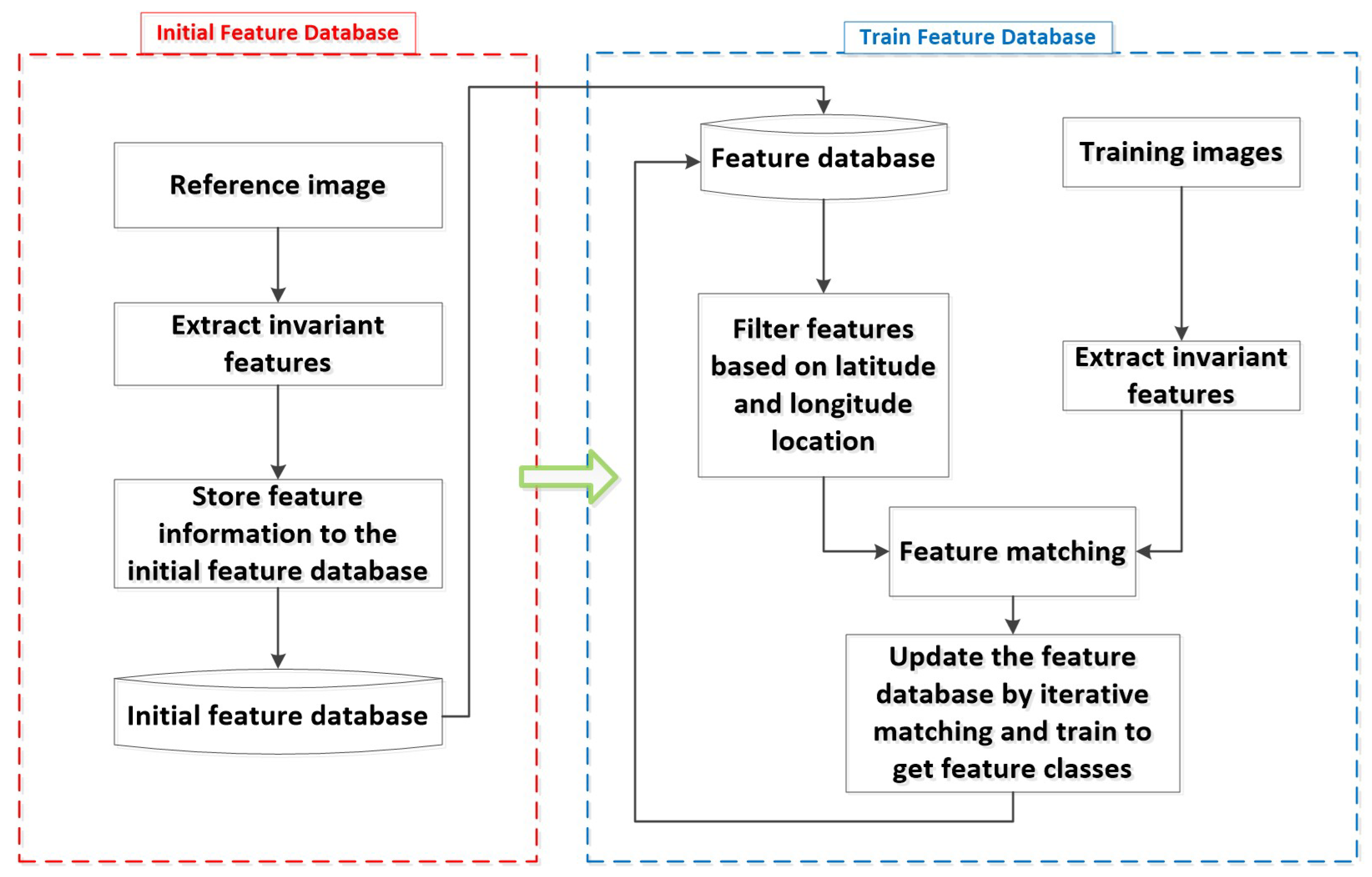
2.2.1. Initial Feature Database Building
| Algorithm 1: Feature Database Construction |
Input: reference image R, training images , the threshold of not matched, , the threshold of consecutive unmatched, Output: feature database |
 |
2.2.2. Iterative Matching Strategy for Feature Database Methods
- A.
- Training image feature set extraction: The training image set is input in temporal order to match the feature database, where N is the number of training images in the training set. When the kth training image is input, the training image is first pre-processed with adaptive histogram equalization, then the feature set is read from the feature database according to the latitude and longitude of the training image, and then the feature set is extracted from the training image using the same feature extraction method as the extraction of the reference image features, where is the number of feature classes in and is the number of feature classes in .
- B.
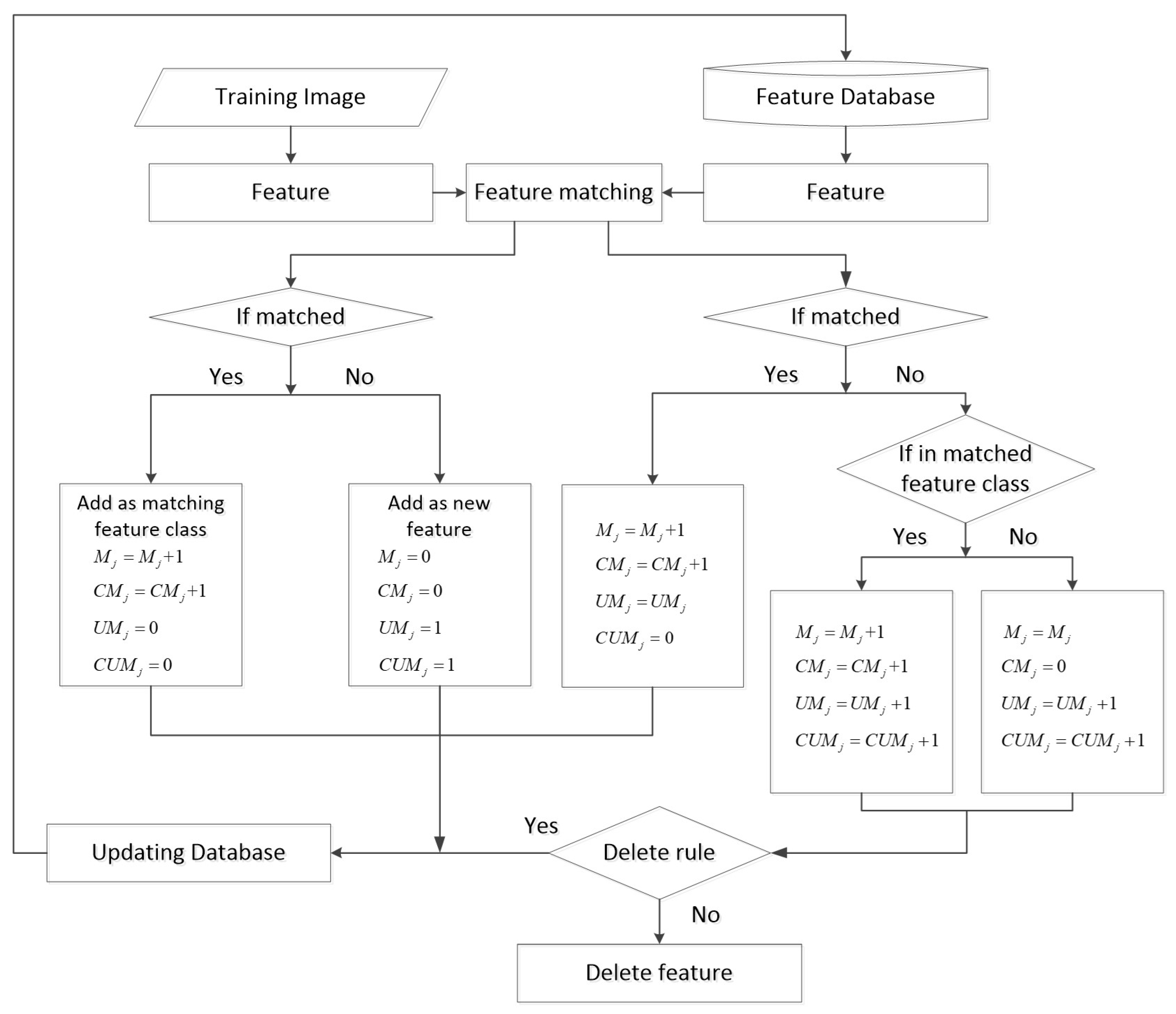
- Feature database feature set update: Feature matching is performed in the feature database set and the training image set . We use the nearest-neighbor distance ratio (NNDR) [14] method based on descriptor distance to select the correspondence, and then the fast sample consensus (FSC) [33] technique is used to filter error matching [34]. Different distance matching methods are used for different feature algorithms, such as KAZE, SIFT, and SURF, which use Euclidean distance matching, and ORB, FREAK, and AKAZE, which use Hamming distance matching. In this paper, image blocks are matched with the feature database and then the number of matched feature points or feature classes exceeds 10 after FSC filtering is considered stable matching, and the matching results are regarded valid. The following step is a modification of based on the matching results of and on the basis of valid matching.
- The feature points successfully matched in :The matching parameters of the feature j in are updated directly, the number of matches is increased by one, , the number of consecutive matches is increased by one, , the number of unmatched matches remains unchanged, , and the number of consecutive unmatched matches is reduced to zero, .
- Feature points in that failed to match:The matching parameters are updated according to the label of the unmatched feature j in . If there is a successful matching point with the same label as the feature j, it means that the feature class of the feature j is successfully matched, but the feature j is not successfully matched; at this time, the number of matches is increased by one, , the number of consecutive matches is increased by one, , the number of unmatched points is increased by one, , and the number of consecutive unmatched points is increased by one, . If there is no successful matching point with the same label, the number of matches remains unchanged, , the number of consecutive matches is cleared, , the number of unmatched matches increases by one, , and the number of consecutive unmatched matches is increased by one, .
- The feature points successfully matched in :In , the matched feature j belongs to a feature class of . After correcting the position according to the matching result, the feature j is added to with the same , and changed to the same as the matched features in , with zero unmatched, and zero consecutive unmatched, .
- Feature points in that failed to match:The unmatched feature j in , after correcting the position according to the matching result, will also be added to the feature database set with a new for the newly added feature, the number of matches and consecutive matches is 0, , and the number of unmatched and consecutive unmatched is 1, , which corresponds to the newly added feature points.
- For other features that are not in the extracted feature set but exist in the feature database, they remain unchanged in the feature database.
- C.
- Delete feature points within the feature set based on the threshold: After the above steps, the features are filtered for , and when the proportion of unmatched times between them to the total number of all training at that point exceeds a threshold, , or when the number of consecutive unmatched times exceeds a threshold, , the features are removed from the feature set . In this paper, we empirically set the parameters and to rewrite the filtered feature set into the feature database.
- D.
- Repeat the above process to iteratively train the feature images: The feature database is continuously updated and iterated using training images, in which feature points that can be matched multiple times are automatically clustered to obtain stable feature classes with the same label, which is equivalent to aggregating multiple feature descriptors at the same location under multiple observation conditions, thus realizing the training process of the feature database.
3. Experiments and Results
3.1. Evaluation Indicators
- 1.
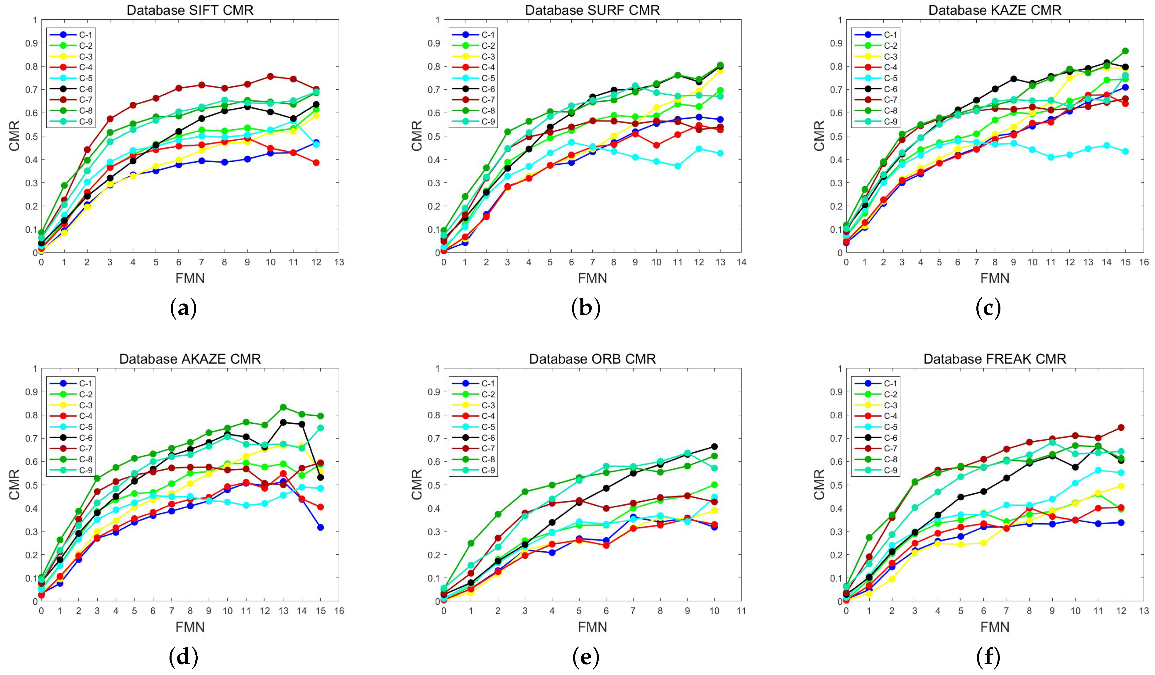
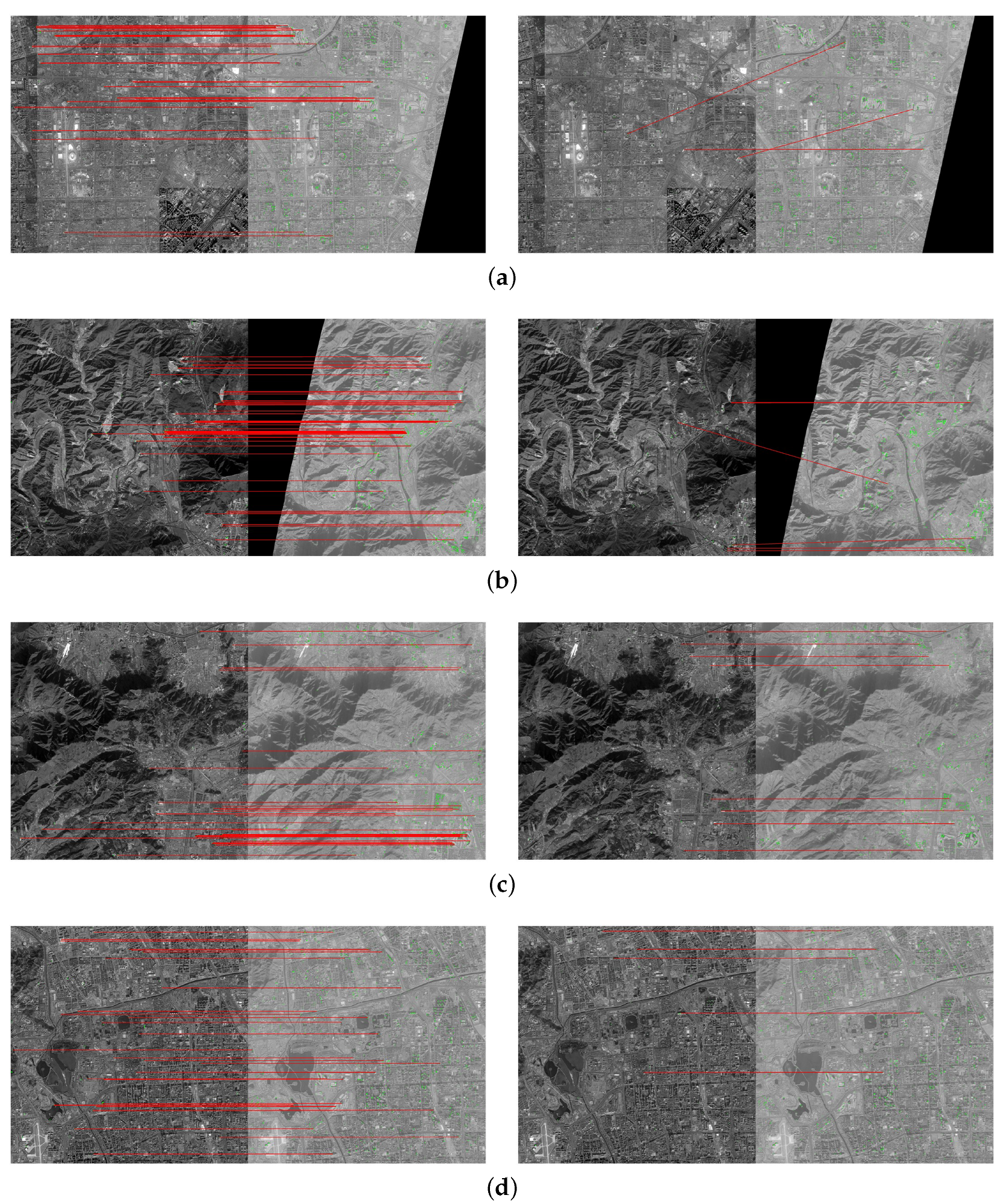
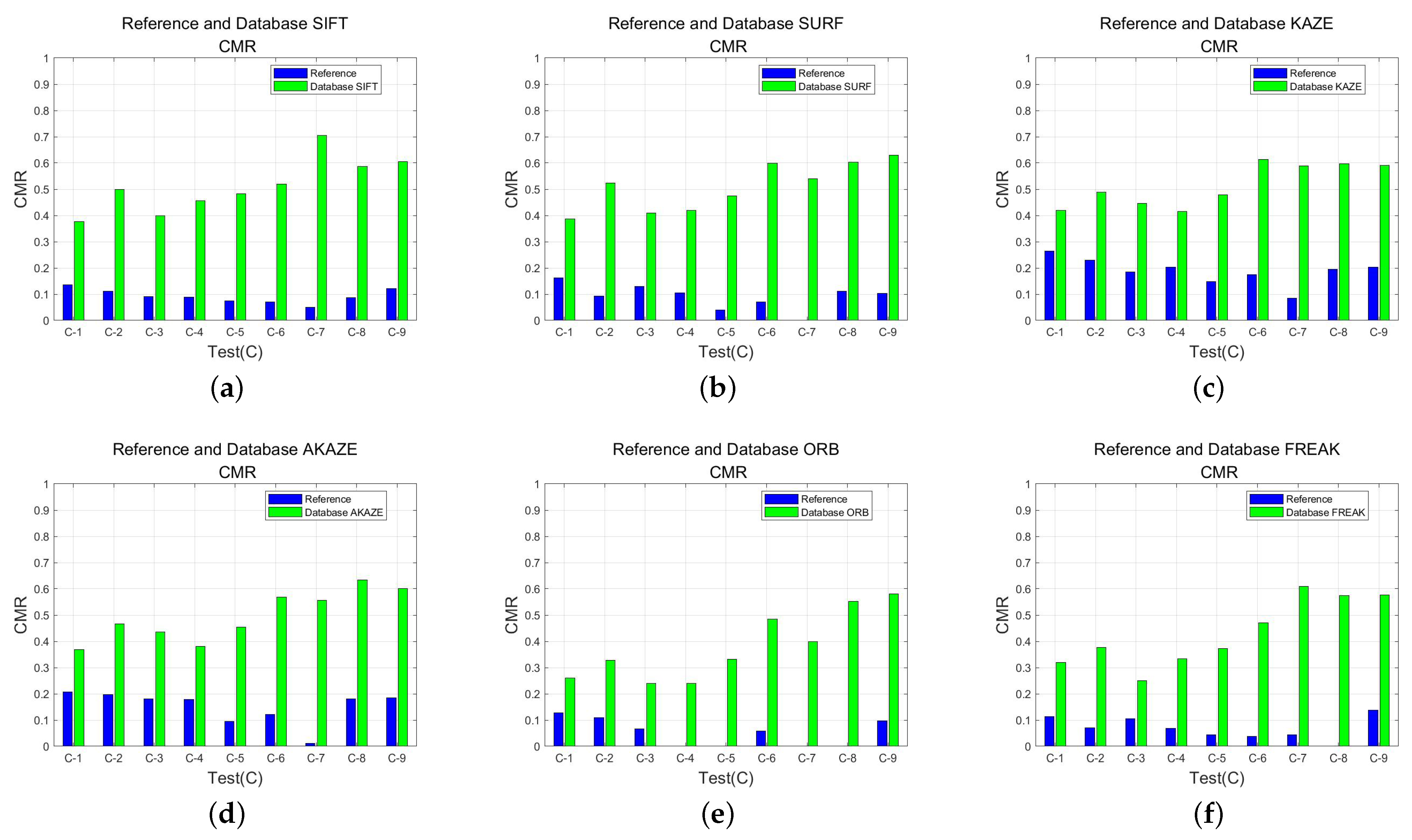
- The stability of the feature matching method is measured by the correct matching ratio (). It is the proportion of the number of correct matches () to the total number of feature matches (). Because a feature class in the feature database matching method contains multiple similar features and a successful match of one of the features means a successful match of this feature class, the calculation of the matching method of the feature database is based on the feature classes described in this paper.
- 2.
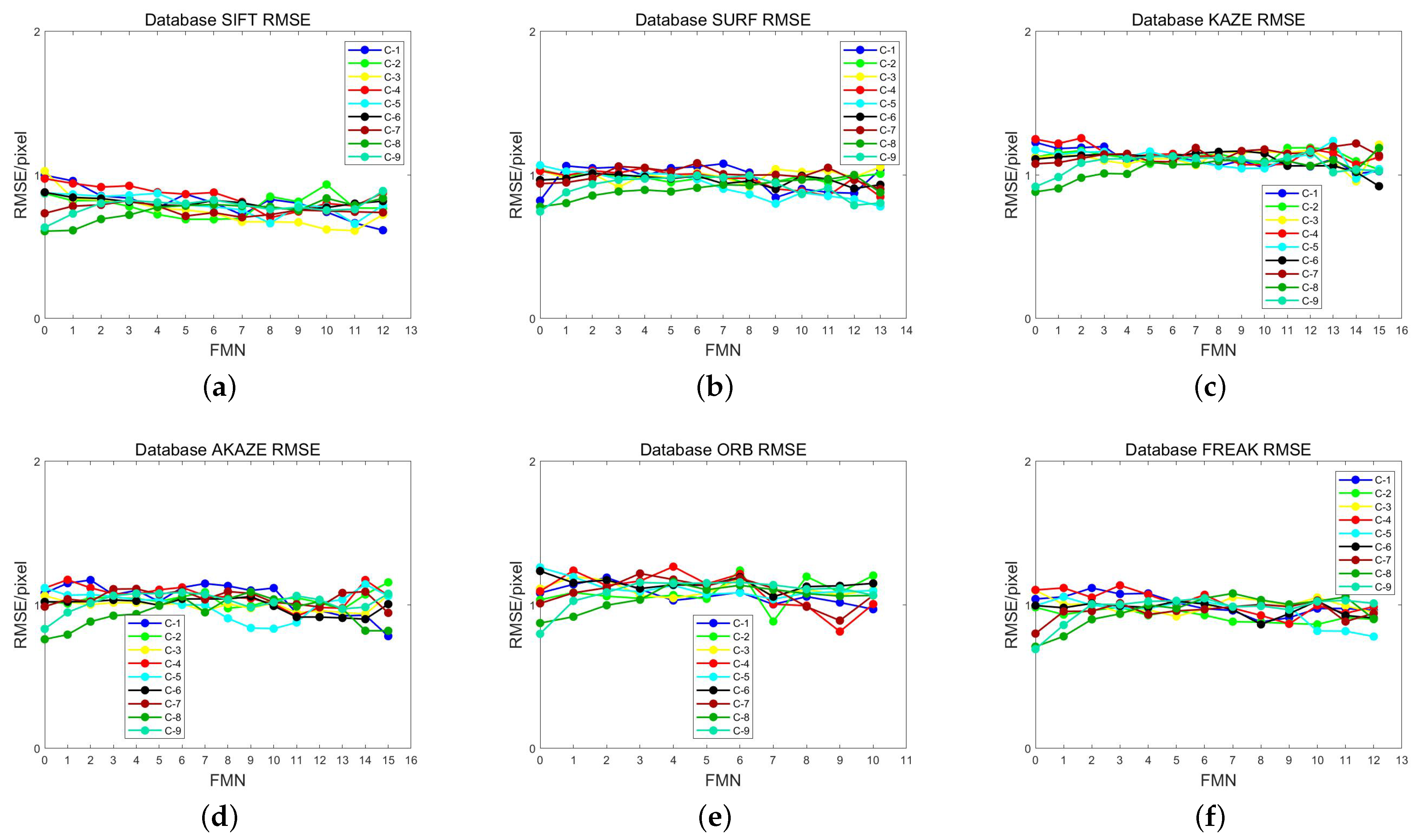
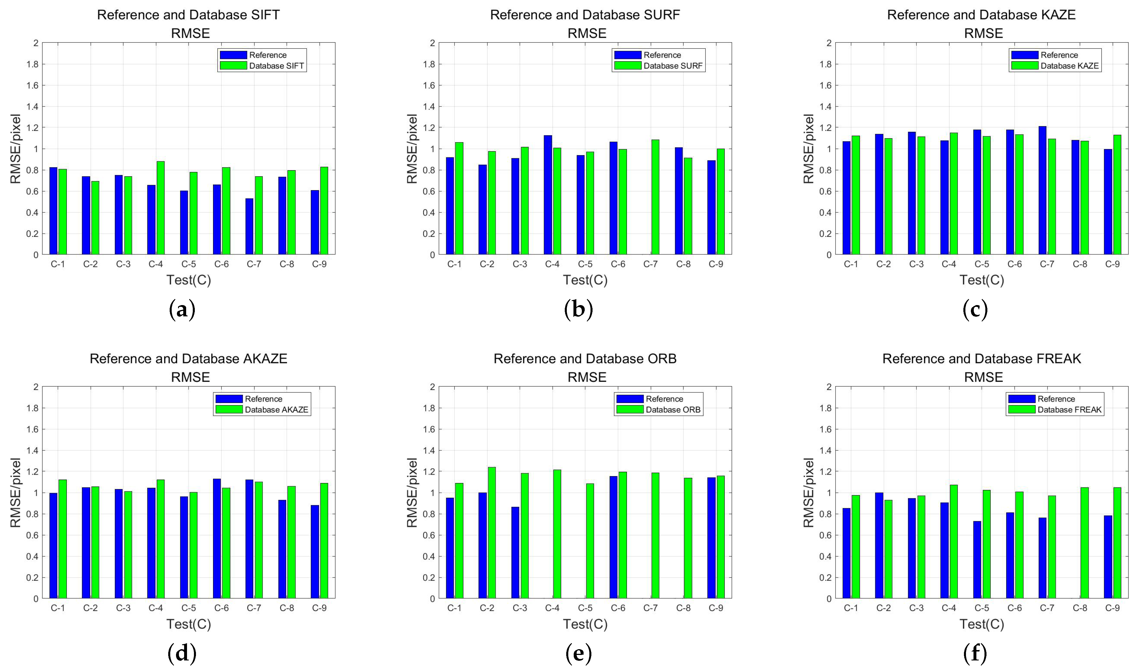
- Root mean square error (), which is used to reflect the geometric localization accuracy of the feature matching method, where denotes the coordinates of the matched feature points in the reference image or feature database and denotes the corresponding coordinates of the matched points in the test image after geometric correction. A smaller denotes a higher degree of geometric localization accuracy using the feature-matching approach.
- 3.
- The total time () spent to extract features and perform feature matching from the reference image or feature database and the test image, which is used to reflect the matching efficiency of the feature matching method.
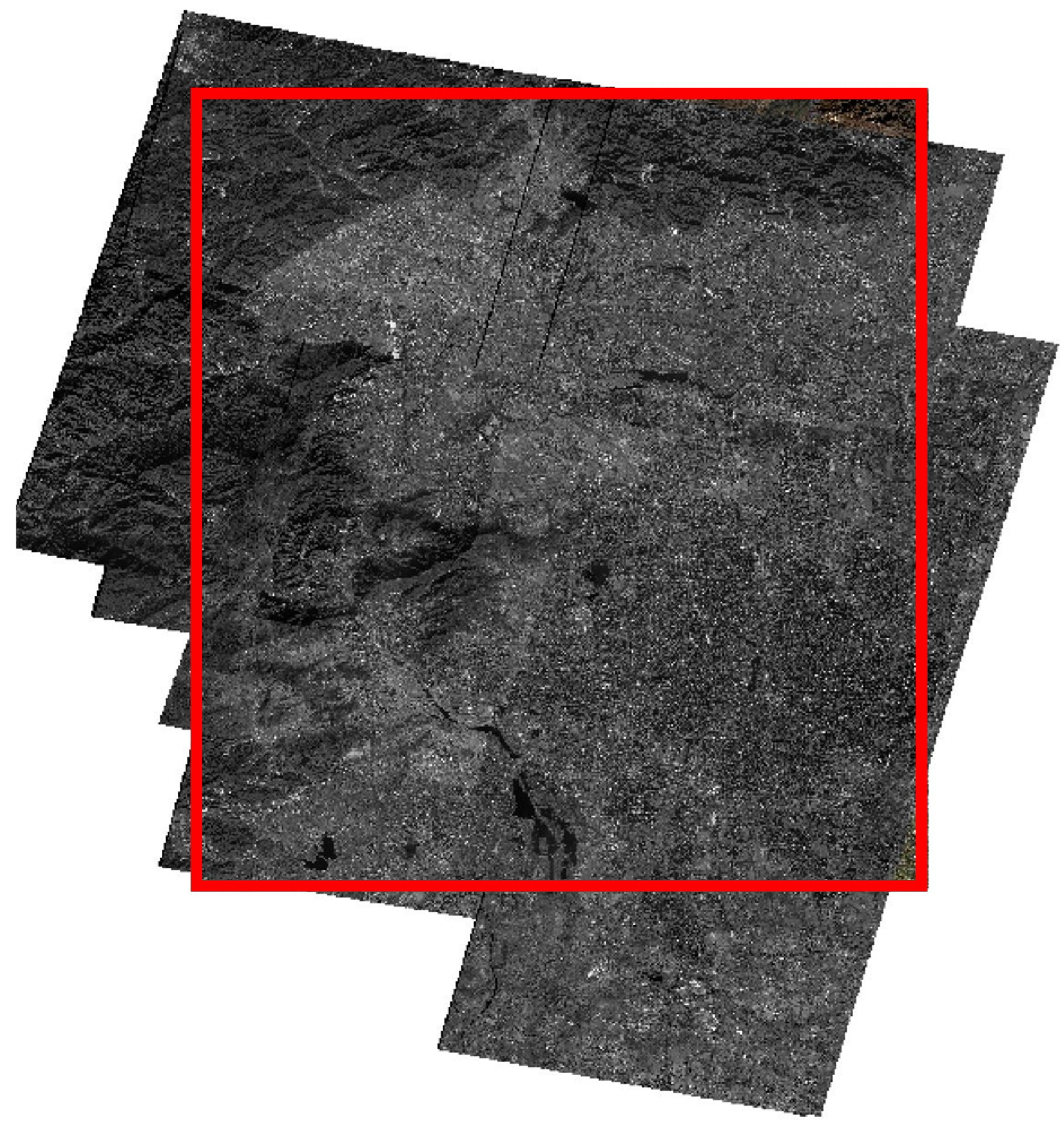
3.2. Experimental Data
3.3. Large Area Remote Sensing Image Feature Database Matching Experiment
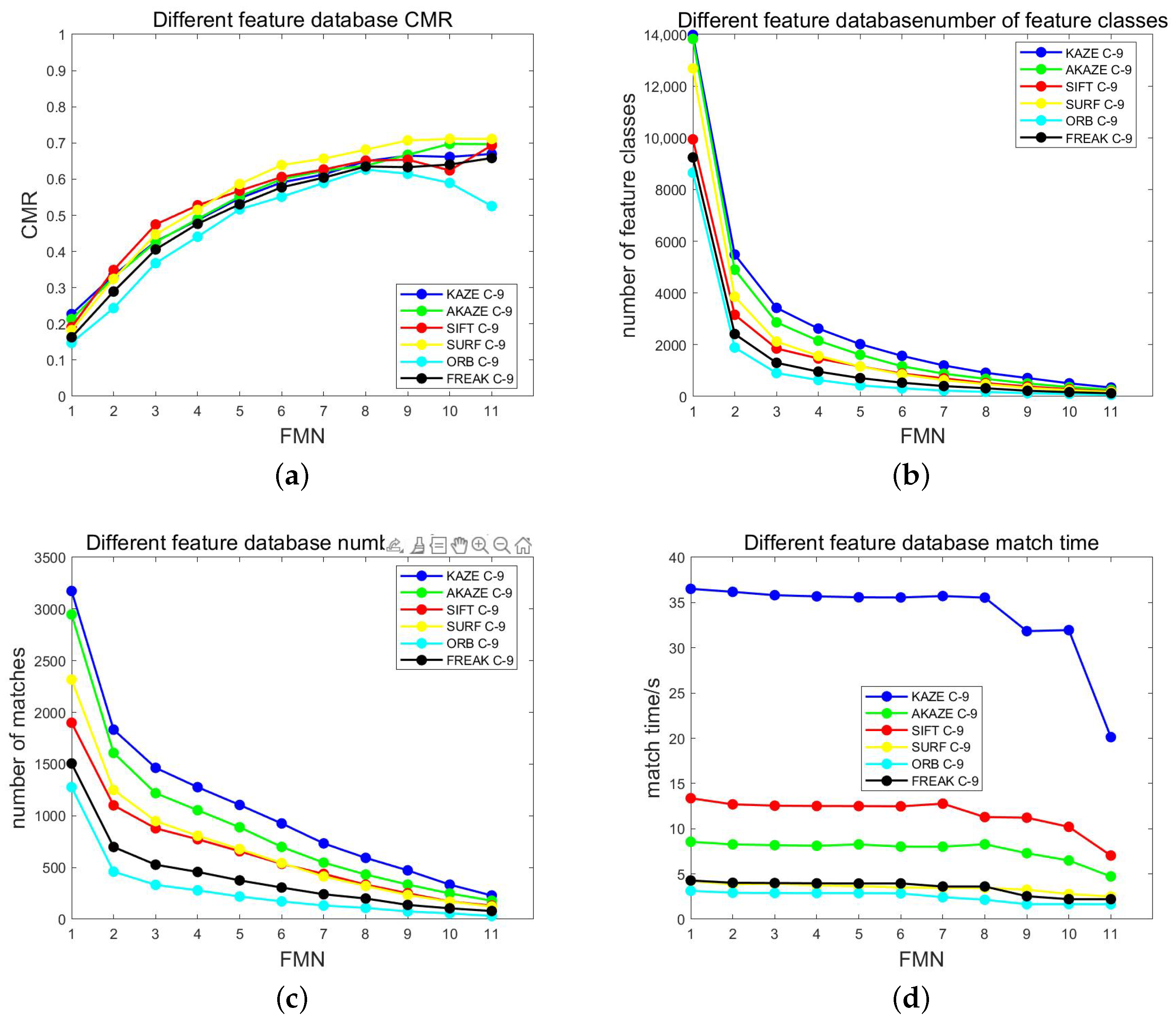
3.3.1. Matching Times Filtering Experiment
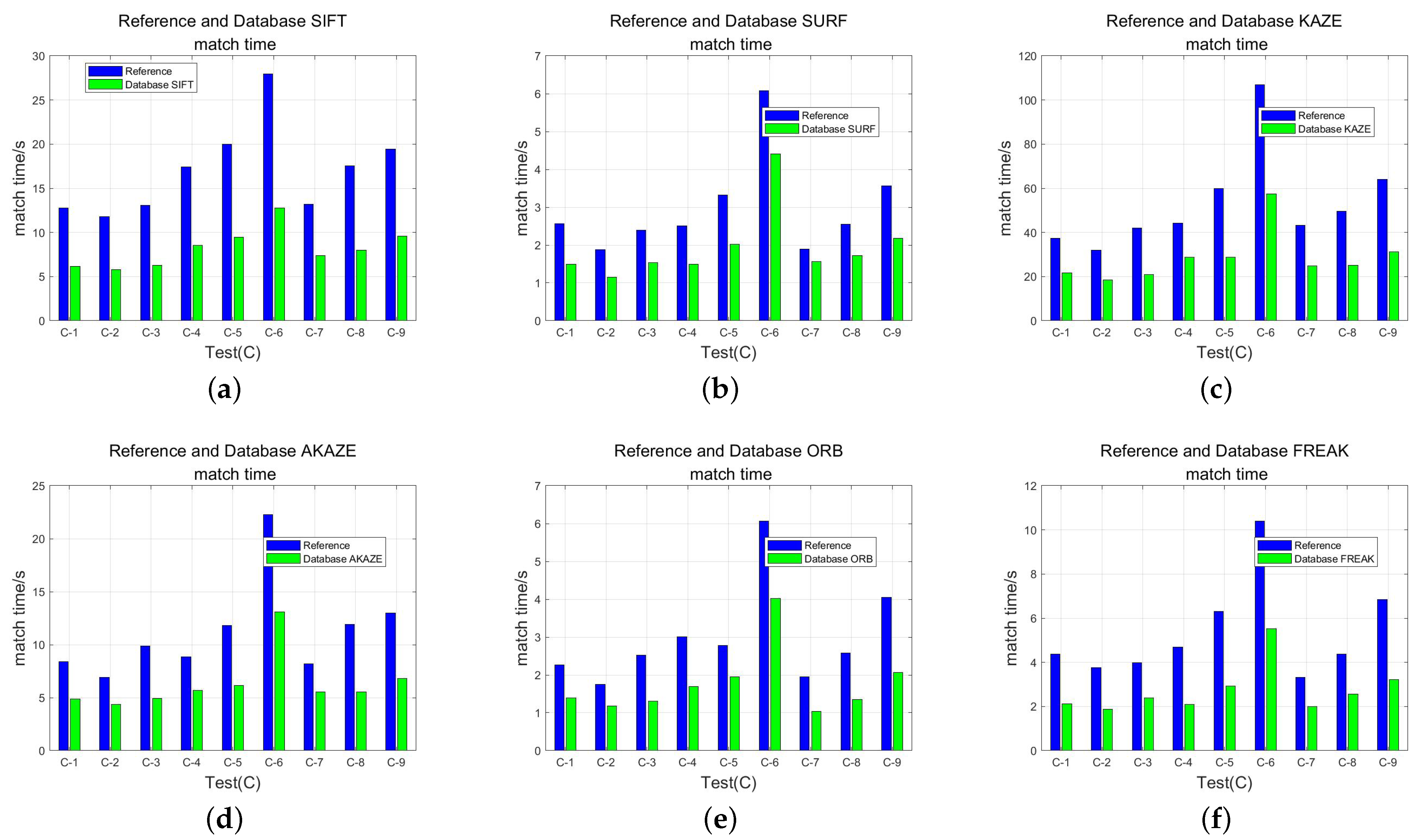
3.3.2. Comparison Experiment between Direct Matching and Feature Database Matching
3.3.3. Difference between Feature Database
4. Discussion
5. Conclusions
- 1.
- Simplicity: This feature database matching method stores the features extracted from the reference image in the feature database simply and effectively for subsequent matching. Since features do not need to be extracted from the reference data each time matching is performed, this reduces the amount of storage space required for the reference data and speeds up geometric correction and remote sensing image matching.
- 2.
- Stability: The feature database extracts features from images of the same region with different time phases and trains stable invariant features (constructs invariant feature point sets) by iterative matching. It increases the correct matching rate by extracting stable feature classes with numerous matches, being adaptable to remote sensing image matching under multiple observation conditions.
- 3.
- Scalability: The method in this paper has good reconfigurability because, in addition to the feature algorithms mentioned in the paper, other feature algorithms can be modified by the image resolution of remote sensing images, various geomorphological features of the target area, and various sensor types for acquiring images. The feature database matching technique can be made even more effective in the future by including faster feature algorithms.
Author Contributions
Funding
Institutional Review Board Statement
Informed Consent Statement
Data Availability Statement
Acknowledgments
Conflicts of Interest
References
- Yue, Z.; Fan, D.; Dong, Y.; Ji, S.; Li, D. A generation method of spaceborne lightweight and fast matching. J. Geo-Inf. Sci. 2022, 24, 925–939. [Google Scholar]
- Zhou, G.; Zhang, R.; Liu, N.; Huang, J.; Zhou, X. On-Board Ortho-Rectification for Images Based on an FPGA. Remote Sens. 2017, 9, 874. [Google Scholar] [CrossRef] [Green Version]
- Chen, B.; Huang, B.; Xu, B. Comparison of Spatiotemporal Fusion Models: A Review. Remote Sens. 2015, 7, 1798–1835. [Google Scholar] [CrossRef] [Green Version]
- Shen, H.; Meng, X.; Zhang, L. An Integrated Framework for the Spatio–Temporal–Spectral Fusion of Remote Sensing Images. IEEE Trans. Geosci. Remote Sens. 2016, 54, 7135–7148. [Google Scholar] [CrossRef]
- Thomas, C.; Ranchin, T.; Wald, L.; Chanussot, J. Synthesis of Multispectral Images to High Spatial Resolution: A Critical Review of Fusion Methods Based on Remote Sensing Physics. IEEE Trans. Geosci. Remote Sens. 2008, 46, 1301–1312. [Google Scholar] [CrossRef] [Green Version]
- Ma, Y.; Li, H.; Gu, H. A Study of Fast Change Detection Algorithm Based on Feature Library of Remote Sensing Imagery. In Proceedings of the 2011 International Symposium on Image and Data Fusion, Tengchong, China, 9–11 August 2011; pp. 1–3. [Google Scholar] [CrossRef]
- Zhang, C.; Feng, Y.; Hu, L.; Tapete, D.; Pan, L.; Liang, Z.; Cigna, F.; Yue, P. A Domain Adaptation Neural Network for Change Detection with Heterogeneous Optical and SAR Remote Sensing Images. Int. J. Appl. Earth Obs. Geoinf. 2022, 109, 102769. [Google Scholar] [CrossRef]
- Zhong, Y.; Liu, W.; Zhao, J.; Zhang, L. Change Detection Based on Pulse-Coupled Neural Networks and the NMI Feature for High Spatial Resolution Remote Sensing Imagery. IEEE Geosci. Remote Sens. Lett. 2015, 12, 537–541. [Google Scholar] [CrossRef]
- Chen, Z.; Chi, Z.; Zinglersen, K.B.; Tian, Y.; Wang, K.; Hui, F.; Cheng, X. A New Image Mosaic of Greenland Using Landsat-8 OLI Images. Sci. Bull. 2020, 65, 522–524. [Google Scholar] [CrossRef] [Green Version]
- Jiang, Y.; Xu, K.; Zhao, R.; Zhang, G.; Cheng, K.; Zhou, P. Stitching Images of Dual-Cameras Onboard Satellite. ISPRS J. Photogramm. Remote Sens. 2017, 128, 274–286. [Google Scholar] [CrossRef]
- Li, X.; Hui, N.; Shen, H.; Fu, Y.; Zhang, L. A Robust Mosaicking Procedure for High Spatial Resolution Remote Sensing Images. ISPRS J. Photogramm. Remote Sens. 2015, 109, 108–125. [Google Scholar] [CrossRef]
- Chen, Q.H.; Liu, X.G.; Gao, W.; Liu, T.L. An Automatic Ground Control Point Matching Based on GCP Chip Database for Remote Sensing Images. In Proceedings of the 2009 International Conference on Image Analysis and Signal Processing, Linhai, China, 11–12 April 2009; pp. 13–17. [Google Scholar] [CrossRef]
- Tang, P.; Zheng, K.; Shan, X.; Hu, C.; Huo, L.; Zhao, L.; Li, H. Framework of remote sensing image automatic processing with “invariant feature point set” as control data set. J. Remote Sens. 2016, 20, 1126–1137. [Google Scholar]
- Lowe, D.G. Distinctive Image Features from Scale-Invariant Keypoints. Int. J. Comput. Vis. 2004, 60, 91–110. [Google Scholar] [CrossRef]
- Ke, Y.; Sukthankar, R. PCA-SIFT: A More Distinctive Representation for Local Image Descriptors. In Proceedings of the 2004 IEEE Computer Society Conference on Computer Vision and Pattern Recognition, Washington, DC, USA, 27 June–2 July 2004; Volume 2, p. II. [Google Scholar] [CrossRef]
- Mikolajczyk, K.; Schmid, C. A Performance Evaluation of Local Descriptors. IEEE Trans. Pattern Anal. Mach. Intell. 2005, 27, 1615–1630. [Google Scholar] [CrossRef] [Green Version]
- Bay, H.; Tuytelaars, T.; Van Gool, L. SURF: Speeded Up Robust Features. In Proceedings of the Computer Vision—ECCV, Graz, Austria, 7–13 May 2006; Lecture Notes in Computer, Science. Leonardis, A., Bischof, H., Pinz, A., Eds.; Springer: Berlin/Heidelberg, Germany, 2006; pp. 404–417. [Google Scholar] [CrossRef]
- Sedaghat, A.; Mokhtarzade, M.; Ebadi, H. Uniform Robust Scale-Invariant Feature Matching for Optical Remote Sensing Images. IEEE Trans. Geosci. Remote Sens. 2011, 49, 4516–4527. [Google Scholar] [CrossRef]
- Alcantarilla, P.F.; Bartoli, A.; Davison, A.J. KAZE Features. In Proceedings of the Computer Vision—ECCV, Florence, Italy, 7–13 October 2012; Lecture Notes in Computer, Science. Fitzgibbon, A., Lazebnik, S., Perona, P., Sato, Y., Schmid, C., Eds.; Springer: Berlin/Heidelberg, Germany, 2012; pp. 214–227. [Google Scholar] [CrossRef]
- Alcantarilla, P.; Nuevo, J.; Bartoli, A. Fast Explicit Diffusion for Accelerated Features in Nonlinear Scale Spaces. In Proceedings of the British Machine Vision Conference, Bristol, UK, 9–13 September 2013; British Machine Vision Association: Bristol, UK, 2013; pp. 13.1–13.11. [Google Scholar] [CrossRef] [Green Version]
- Rublee, E.; Rabaud, V.; Konolige, K.; Bradski, G. ORB: An Efficient Alternative to SIFT or SURF. In Proceedings of the 2011 International Conference on Computer Vision, Barcelona, Spain, 6–13 October 2011; pp. 2564–2571. [Google Scholar] [CrossRef]
- Leutenegger, S.; Chli, M.; Siegwart, R.Y. BRISK: Binary Robust Invariant Scalable Keypoints. In Proceedings of the 2011 International Conference on Computer Vision, Barcelona, Spain, 6–13 October 2011; pp. 2548–2555. [Google Scholar] [CrossRef] [Green Version]
- Alahi, A.; Ortiz, R.; Vandergheynst, P. FREAK: Fast Retina Keypoint. In Proceedings of the 2012 IEEE Conference on Computer Vision and Pattern Recognition, Providence, RI, USA, 16–21 June 2012; pp. 510–517. [Google Scholar] [CrossRef] [Green Version]
- Ma, J.; Jiang, J.; Zhou, H.; Zhao, J.; Guo, X. Guided Locality Preserving Feature Matching for Remote Sensing Image Registration. IEEE Trans. Geosci. Remote Sens. 2018, 56, 4435–4447. [Google Scholar] [CrossRef]
- Li, Z.; Yue, J.; Fang, L. Adaptive Regional Multiple Features for Large-Scale High-Resolution Remote Sensing Image Registration. IEEE Trans. Geosci. Remote Sens. 2022, 60, 1–13. [Google Scholar] [CrossRef]
- Chen, S.; Zhong, S.; Xue, B.; Li, X.; Zhao, L.; Chang, C.I. Iterative Scale-Invariant Feature Transform for Remote Sensing Image Registration. IEEE Trans. Geosci. Remote Sens. 2021, 59, 3244–3265. [Google Scholar] [CrossRef]
- Kelman, A.; Sofka, M.; Stewart, C.V. Keypoint Descriptors for Matching Across Multiple Image Modalities and Non-linear Intensity Variations. In Proceedings of the 2007 IEEE Conference on Computer Vision and Pattern Recognition, Minneapolis, MN, USA, 17–22 June 2007; pp. 1–7. [Google Scholar] [CrossRef] [Green Version]
- Martins, P.; Carvalho, P.; Gatta, C. On the Completeness of Feature-Driven Maximally Stable Extremal Regions. Pattern Recognit. Lett. 2016, 74, 9–16. [Google Scholar] [CrossRef]
- Ma, W.; Wu, Y.; Liu, S.; Su, Q.; Zhong, Y. Remote Sensing Image Registration Based on Phase Congruency Feature Detection and Spatial Constraint Matching. IEEE Access 2018, 6, 77554–77567. [Google Scholar] [CrossRef]
- Agrawal, M.; Konolige, K.; Blas, M.R. CenSurE: Center Surround Extremas for Realtime Feature Detection and Matching. In Computer Vision—ECCV 2008; Hutchison, D., Kanade, T., Kittler, J., Kleinberg, J.M., Mattern, F., Mitchell, J.C., Naor, M., Nierstrasz, O., Pandu Rangan, C., Steffen, B., Eds.; Springer: Berlin/Heidelberg, Germany, 2008; Volume 5305, pp. 102–115. [Google Scholar] [CrossRef]
- Rosten, E.; Drummond, T. Machine Learning for High-Speed Corner Detection. In Proceedings of the Computer Vision—ECCV, Graz, Austria, 7–13 May 2006; Lecture Notes in Computer, Science. Leonardis, A., Bischof, H., Pinz, A., Eds.; Springer: Berlin/Heidelberg, Germany, 2006; pp. 430–443. [Google Scholar] [CrossRef]
- Calonder, M.; Lepetit, V.; Strecha, C.; Fua, P. BRIEF: Binary Robust Independent Elementary Features. In Proceedings of the Computer Vision—ECCV, Crete, Greece, 5–11 September 2010; Lecture Notes in Computer, Science. Daniilidis, K., Maragos, P., Paragios, N., Eds.; Springer: Berlin/Heidelberg, Germany, 2010; pp. 778–792. [Google Scholar] [CrossRef] [Green Version]
- Wu, Y.; Ma, W.; Gong, M.; Su, L.; Jiao, L. A Novel Point-Matching Algorithm Based on Fast Sample Consensus for Image Registration. IEEE Geosci. Remote Sens. Lett. 2015, 12, 43–47. [Google Scholar] [CrossRef]
- Xiang, Y.; Wang, F.; You, H. OS-SIFT: A Robust SIFT-Like Algorithm for High-Resolution Optical-to-SAR Image Registration in Suburban Areas. IEEE Trans. Geosci. Remote Sens. 2018, 56, 3078–3090. [Google Scholar] [CrossRef]
- Moghimi, A.; Celik, T.; Mohammadzadeh, A.; Kusetogullari, H. Comparison of Keypoint Detectors and Descriptors for Relative Radiometric Normalization of Bitemporal Remote Sensing Images. IEEE J. Sel. Top. Appl. Earth Obs. Remote Sens. 2021, 14, 4063–4073. [Google Scholar] [CrossRef]
- Ye, Y.; Shan, J.; Bruzzone, L.; Shen, L. Robust Registration of Multimodal Remote Sensing Images Based on Structural Similarity. IEEE Trans. Geosci. Remote Sens. 2017, 55, 2941–2958. [Google Scholar] [CrossRef]
- Li, J.; Hu, Q.; Ai, M. RIFT: Multi-Modal Image Matching Based on Radiation-Variation Insensitive Feature Transform. IEEE Trans. Image Process. 2020, 29, 3296–3310. [Google Scholar] [CrossRef]


| Algorithm | Detector Type | Description |
|---|---|---|
| SIFT | Blobs | SIFT first constructs the Difference-of-Gaussian scale space based on the Gaussian scale space; next, the keypoints are detected and precisely located in the Difference-of-Gaussian images; after that, one or more orientations are determined by the peak of the gradient histogram of each key point neighborhood. Finally, 128-dimensional feature descriptors are constructed based on the gradient information of the neighborhood centered on the keypoints. |
| SURF | Blobs | SURF uses box filters to convolve with the original image to construct the scale space while using the integral image technique to increase the computational efficiency of the algorithm. It detects the candidate feature points using the Hessian Matrix, followed by non-maximal suppression. To determine the keypoint orientation, SURF adds up the Haar-wavelet responses in the horizontal and vertical orientation of the angular sector sliding window in the circular neighborhood of the keypoint. The orientation of the longest such vector sum is used as the keypoint orientation. Furthermore, SURF statistics the Haar-wavelet responses in the area around the keypoint to create a 64-dimensional feature descriptor. |
| KAZE | Blobs | KAZE uses efficient Additive Operator Splitting (AOS) techniques for nonlinear diffusion filtering to build nonlinear scale space, which reduces noise while maintaining edges. It searches for Hessian local maxima on the nonlinear scale space after normalization at different scales as the keypoint and finds the dominant orientations of feature points in a similar way to SURF. KAZE builds the descriptor using a variant of the SURF descriptor, Modified-SURF (M-SURF) [30], which can handle the boundaries better than the original SURF descriptor and finally forms a 64-dimensional feature vector. |
| AKAZE | Blobs | AKAZE is an accelerated variant of KAZE. It constructs nonlinear scale spaces more quickly by using the Fast Explicit Diffusion (FED) mathematical framework. Similar to KAZE, It locates candidate points and filters them at each octave to perform keypoint extraction. It calculates the dominant orientations of keypoints in a similar way to KAZE. It uses an updated Modified-Local Difference Binary (M-LDB) binary descriptor for descriptor construction that not only compares region means instead of individual pixels in the binary set but also incorporates rotation invariance. |
| ORB | Corners | ORB consists of a modified FAST (Features from Accelerated Segment Test) [31] and a rotated BRIEF (Binary Robust Independent Elementary Features) [32]. It first uses FAST to quickly select keypoints; afterward, it uses the intensity centroid method to calculate keypoint orientations; and finally, it uses the modified BRIEF to create binary descriptors, compared with the original BRIEF descriptors with increased rotational invariance compared with the original BRIEF. |
| FREAK | Corners | Only the descriptor extraction approach is improved by FREAK. The keypoint detection algorithm in BRISK is used in the original paper to perform FAST feature point detection on the constructed multi-scale space. However, unlike the uniform sampling pattern of BRISK for extracting feature descriptors, FREAK is inspired by the human visual system and uses a retinal sampling pattern where the smaller the distance from the keypoint, the denser the sampling, and the larger the distance from the keypoint, the more discrete the sampling points. |
| Control Point Mode | Storage Content | Storage Type | Storage Size/Byte | Total Storage Size/Byte | Compression Ratio |
|---|---|---|---|---|---|
| Control Point | Longitude and Latitude | float | 8 | 40,008 | |
| Local Image (200 × 200) | unsigned char | 40,000 | |||
| SIFT | 128-dimensional Descriptor | float | 512 | 556 | 1/72 |
| Point properties 1, Update parameters 2 | float | 44 | |||
| SURF | 64-dimensional Descriptor | float | 256 | 300 | 1/133 |
| Point properties 1, Update parameters 2 | float | 44 | |||
| KAZE | 64-dimensional Descriptor | float | 256 | 300 | 1/133 |
| Point properties 1, Update parameters 2 | float | 44 | |||
| AKAZE | 64-dimensional Descriptor | unsigned char | 64 | 108 | 1/370 |
| Point properties 1, Update parameters 2 | float | 44 | |||
| ORB | 32-dimensional Descriptor | unsigned char | 32 | 76 | 1/526 |
| Point properties 1, Update parameters 2 | float | 44 | |||
| FREAK | 64-dimensional Descriptor | unsigned char | 64 | 108 | 1/370 |
| Point properties 1, Update parameters 2 | float | 44 |
| Image | Source | Number | Date | Size (Pixel × Pixel) | Resolution (m) |
|---|---|---|---|---|---|
| Reference (A) | Google Earth | 1 | 2016 | 53,120 × 49,152 | 1.19 |
| Training (B) | GF2 | 50 | 2016–2022 | 27,620 × 29,200 | 0.81 |
| Test (C) | JL1 (C-1 C-2 C-3) | 3 | 2019–2020 | 28,651 × 28,720 | 0.75 |
| GF1 (C-4 C-5 C-6) | 3 | 2019–2021 | 18,236 × 18,190 | 2 | |
| GF2 (C-7 C-8 C-9) | 3 | 2019–2021 | 27,620 × 29,200 | 0.81 |
| Algorithm | C-1 | C-2 | C-3 | C-4 | C-5 | C-6 | C-7 | C-8 | C-9 |
|---|---|---|---|---|---|---|---|---|---|
| SIFT | 0.3835 | 0.2424 | 0.4150 | 0.2715 | 0.2144 | 0.1203 | 0.1174 | 0.2299 | 0.2544 |
| SURF | 0.2573 | 0.1032 | 0.1405 | 0.2023 | 0.2872 | 0.1100 | 0.1811 | 0.2214 | 0.2519 |
| KAZE | 0.2178 | 0.1520 | 0.2553 | 0.1853 | 0.2635 | 0.2448 | 0.1415 | 0.3060 | 0.2463 |
| AKAZE | 0.3909 | 0.1901 | 0.1335 | 0.2526 | 0.3090 | 0.1574 | 0.1673 | 0.3305 | 0.2536 |
| ORB | 0.2203 | 0.3554 | 0.1493 | 0.4519 | 0.2214 | 0.1793 | 0.3277 | 0.2868 | 0.3591 |
| FREAK | 0.2366 | 0.1192 | 0.1809 | 0.2683 | 0.2764 | 0.1639 | 0.2306 | 0.3709 | 0.3540 |
| Algorithm | Stable Direct Match/Image | Stable Feature Database Matching/Image | Average CMR Increase/% | RMSE Absolute Difference Mean/pixel | Average Time Reduction/% |
|---|---|---|---|---|---|
| SIFT | 9 | 9 | 42.23 | 0.1251 | 51.31 |
| SURF | 8 | 9 | 40.38 | 0.101 | 36.83 |
| KAZE | 9 | 9 | 32.78 | 0.064 | 45.66 |
| AKAZE | 9 | 9 | 34.54 | 0.0803 | 43.08 |
| ORB | 5 | 9 | 28.76 | 0.1508 | 40.33 |
| FREAK | 8 | 9 | 33.61 | 0.1685 | 48.69 |
Disclaimer/Publisher’s Note: The statements, opinions and data contained in all publications are solely those of the individual author(s) and contributor(s) and not of MDPI and/or the editor(s). MDPI and/or the editor(s) disclaim responsibility for any injury to people or property resulting from any ideas, methods, instructions or products referred to in the content. |
© 2023 by the authors. Licensee MDPI, Basel, Switzerland. This article is an open access article distributed under the terms and conditions of the Creative Commons Attribution (CC BY) license (https://creativecommons.org/licenses/by/4.0/).
Share and Cite
Zhao, Z.; Long, H.; You, H. An Optical Remote Sensing Image Matching Method Based on the Simple and Stable Feature Database. Appl. Sci. 2023, 13, 4632. https://doi.org/10.3390/app13074632
Zhao Z, Long H, You H. An Optical Remote Sensing Image Matching Method Based on the Simple and Stable Feature Database. Applied Sciences. 2023; 13(7):4632. https://doi.org/10.3390/app13074632
Chicago/Turabian StyleZhao, Zilu, Hui Long, and Hongjian You. 2023. "An Optical Remote Sensing Image Matching Method Based on the Simple and Stable Feature Database" Applied Sciences 13, no. 7: 4632. https://doi.org/10.3390/app13074632