Ship Defense Strategy Using a Planar Grid Formation of Multiple Drones

Abstract

This article introduces a ship defense strategy using a planar grid formation of multiple drones. We handle a scenario where a high-speed target with variable velocity heads towards the ship. The ship measures the position of the target in real time. Based on the measured target, the drones guidance laws are calculated by the ships on-board computer and are sent to every drone in real time. The drones form a planar grid formation, whose center blocks the Line-Of-Sight (LOS) line connecting the target and the ship. Since the target is guided to hit its goal (ship), the drones can effectively block the target by blocking the LOS line. We enable slow drones to capture a fast target by making the drones stay close to the ship while blocking the LOS at all times. By using a grid formation of drones, we can increase the capture rate, even when there exists error in the prediction of the target’s position. To the best of our knowledge, this article is unique in using a formation of multiple drones to intercept a fast target with variable velocity. Through MATLAB simulations, the effectiveness of our multi-agent guidance law is verified by comparing it with other state-of-the-art guidance controls.

1. Introduction

This article introduces a ship defense strategy using a clustered formation of multiple drones. We handle a scenario where a high-speed target with variable velocity heads towards the ship. The role of the drone team is to protect the ship from the incoming target.

We propose a ship defense approach with multiple drones, such that each drone is not equipped with powerful sensors or an on-board computer. Thus, a drone cannot measure the target, and the target moves based on the commands sent by the ship. In this way, we can decrease the cost of a drone, which can be destroyed once it intersects the target. This enables us to develop rather cheap drones.

Instead, the ship measures the position of the target in real time. Position measurements can be provided by various sensors, such as radar, IR, or laser sensors of the ship. Each drone’s guidance law is calculated by the ship’s on-board computer and is transmitted to each drone in real time. (This approach relies on the communication between the ship and a drone. Since the signal speed is sufficiently fast ($3\times {10}^8$ m/s) in the air, we argue that signal delay is negligible in our ship defense scenario.)

Consider a high-speed target whose goal is to hit a ship. The target heads towards its goal (ship) at least in the terminal phase. Otherwise, it is impossible to make a target hit the ship.

Therefore, this paper lets multiple drones form a planar grid formation, whose center lies on the line segment connecting the target and the ship. Moreover, the planar grid formation is generated to be perpendicular to the line segment connecting the target and the formation center. The grid formation can be considered as a “net” structure for capturing the incoming target. The target may perform elusive maneuvers, and there may be measurement noise in measuring the target position. By maximizing the grid formation size, we can increase the capture rate, even when there exists error in the prediction of the target’s position. Since the target is guided to hit its goal (ship), the drones can effectively block the target using this grid formation.

As an interceptor, we consider a highly maneuverable drone, such as a quadrotor drone [1,2,3], which is much slower than the incoming target. This article addresses a high-level path planner, which generates reference position signals for a low-level controller [1,2,3].

To the best of our knowledge, our paper is novel in developing a ship defense approach using clustered multiple drones. Our paper is novel in addressing a 3D formation of multiple drones for intercepting a high-speed target with variable speeds. We show that in the case where the drones block the LOS line between the target and the ship, the target cannot reach the ship without being captured by the drones. Since the target is guided to hit its goal (ship), the drones can effectively block the target using this strategy. We further let slow drones stay close to the ship in order to protect the ship from the fast target. As far as we know, our paper is novel in showing that slow drones can capture a fast target by staying close to the ship while blocking the LOS at all times.

Our paper is unique in capturing a maneuvering target with variable speeds, which can be faster than the interceptors. In order to estimate the pose of a maneuvering high-speed target, we applied target-tracking filters in [4]. We control the drone formation, based on the prediction of the target’s position after one sample-index in the future. This prediction may be erroneous due to the target’s elusive maneuvers or measurement noise. This is the motivation for utilizing a grid formation of drones instead of a single drone. Since we use a grid formation, we can increase the capture rate even when the target prediction is erroneous. By maximizing the grid formation size, we can increase the capture rate even when there exists error in the prediction of the target’s position.

To the best of our knowledge, our paper is novel in the following aspects:

• We develop a ship defense approach using clustered multiple drones;
• We use a 3D formation of multiple drones for intercepting a high-speed target with variable speeds;
• We let the drones stay close to the ship while blocking the LOS between the ship and the target. Thus, we enable slow drones to capture a fast target.

Through MATLAB simulations, the effectiveness of our multi-agent guidance law is verified by comparing it with other state-of-the-art guidance controls.

We organize this article as follows. Section 2 addresses the literature review of this paper. Section 3 addresses the preliminary information of this paper. Section 4 discusses several definitions and assumptions in this article. Section 5 introduces our multi-agent guidance law. Section 6 shows simulation results to present the effectiveness of the proposed guidance law. Section 7 provides a conclusion.

2. Literature Review

There are many papers on interceptors’ guidance laws [5,6,7,8]. The authors of [9,10,11,12,13,14,15,16] applied motion camouflage to develop the guidance law of an interceptor. Here, we say that the interceptor is in the motion camouflage state if an interceptor moves in the presence of a target while appearing stationary at a focal point.

References [17,18] developed a motion camouflage guidance law so that the interceptor approaches the target while appearing stationary at a focal point that is infinitely far from the interceptor. The authors of [19] used a neural network architecture to perform motion camouflage in 2D environments. The authors of [12] developed an optimal control approach to derive a 2D motion camouflage position for an interceptor, assuming there is a constant velocity (speed and heading) target. However, assuming a target with constant velocity is not realistic since a maneuvering target could escape from the interceptor. Our paper thus handles a target with variable velocity.

Proportional Navigation Guidance (PNG) laws have been widely applied to let an interceptor hit the target [20,21,22,23]. PNG laws are designed considering an interceptor that can measure the bearing of the target by utilizing on-board sensors. PNG laws are based on the fact that two vehicles are on a collision course when their direct Line-Of-Sight (LOS) does not change direction as they get closer to each other. PNG laws are designed so that the interceptor velocity vector rotates at a rate proportional to the rotation rate of the line-of-sight and in the same direction.

Multi-agent systems can be applied for many tasks, such as monitoring environments [24,25], multi-agent herding [26], and sensor deployment [27,28,29,30]. References [31,32] controlled multiple mobile sensors to estimate the target position in real time. References [33,34] considered the case where two interceptors, which measure bearings of a target, track the target in two dimensions. The formulation of the homing problem of multiple missiles against a single target, subject to constraints on the impact time, was discussed in [35]. In [36], a fully distributed adaptive method was proposed to solve the simultaneous attack problem with multiple missiles against maneuvering targets. The authors of [37] considered the relative interception angle constraints of multiple interceptors, which is intended to enhance the survivability of multiple interceptors against a defense system with a high value target and also to maximize the collateral target damage. The authors of [38] addressed simultaneous cooperative interception for a scenario where the successful handover cannot be guaranteed by a single interceptor due to the target maneuver and movement information errors at the handover moment.

As far as we know, other guidance laws in the literature make one or more interceptors continue to chase the target. Our paper is unique in making slow interceptors (drones in our paper) stay close to the ship, so they can block a fast target from reaching the ship. This blocking strategy is desirable considering the energy consumption of an interceptor since an interceptor does not have to move far from the ship. Through MATLAB simulations, the effectiveness of this blocking strategy is verified by comparing it with other state-of-the-art guidance controls.

3. Preliminaries

This article utilizes two frames: an inertial reference frame $\left\{I\right\}$ and a body-fixed frame $\left\{B\right\}$ [39]. We address several definitions in rigid-body dynamics [39].

The origin of $\left\{I\right\}$ is a point with three axes pointing North, East, and Down, respectively. We use the virtual agent for drone controls. The virtual agent is a virtual drone located at the center of the grid formation. $\left\{B\right\}$ is fixed to the virtual agent, such that the origin of $\left\{B\right\}$ is at the virtual agent’s center.

The virtual agent changes its yaw and pitch while not rotating its body. In rigid-body dynamics [39], $\theta$ and $\psi$ define pitch and yaw, respectively. For convenience, let $c\left(\eta \right)$ define $cos\left(\eta \right)$. In addition, let $s\left(\eta \right)$ define $sin\left(\eta \right)$. Let $t\left(\eta \right)$ define $tan\left(\eta \right)$.

The rotation matrix indicating the counterclockwise (CC) rotation of an angle $\psi$ centered at the z-axis in $\left\{B\right\}$ is

$$\begin{array}{c}\hfill {\mathbf{M}}_R\left(\psi \right)=\left(\begin{array}{ccc}c\left(\psi \right)& -s\left(\psi \right)& 0\\ s\left(\psi \right)& c\left(\psi \right)& 0\\ 0& 0& 1\end{array}\right).\end{array}$$

(1)

The rotation matrix representing the CC rotation of an angle $\theta$ centered at the y-axis in $\left\{B\right\}$ is

$$\begin{array}{c}\hfill {\mathbf{M}}_R\left(\theta \right)=\left(\begin{array}{ccc}c\left(\theta \right)& 0& s\left(\theta \right)\\ 0& 1& 0\\ -s\left(\theta \right)& 0& c\left(\theta \right)\end{array}\right).\end{array}$$

(2)

The combined rotation matrix is built by multiplying Equations (1) and (2) to obtain

$$\begin{array}{c}\hfill {\mathbf{M}}_R(\psi ,\theta )={\mathbf{M}}_R\left(\psi \right){\mathbf{M}}_R\left(\theta \right).\end{array}$$

(3)

4. Assumptions and Definitions

This section discusses assumptions and definitions in our paper. $max(a,b)$ returns a bigger value between two variables (a and b). In addition, $min(a,b)$ returns a smaller value between two variables (a and b). In our paper, bold characters are used to denote vectors and matrices. $\angle ({\mathbf{v}}_1,{\mathbf{v}}_2)$ is the angle formed by two vectors (${\mathbf{v}}_1$ and ${\mathbf{v}}_2$). Mathematically, $\angle ({\mathbf{v}}_1,{\mathbf{v}}_2)=arccos\left(\frac{{\mathbf{v}}_1·{\mathbf{v}}_2}{\parallel {\mathbf{v}}_1\parallel \ast \parallel {\mathbf{v}}_2\parallel }\right)$. Here, $0\le \angle ({\mathbf{v}}_1,{\mathbf{v}}_2)\le \pi$. $l(\mathbf{A},\mathbf{B})$ is the line segment connecting two locations $\mathbf{A}$ and $\mathbf{B}$. Furthermore, $\parallel l(\mathbf{A},\mathbf{B})\parallel$ indicates the length of $l(\mathbf{A},\mathbf{B})$.

This article uses the discrete-time system, where T denotes the sample duration. In this article, all drones make a planar grid formation to protect against the incoming target. The grid formation can be considered as a “net” structure for capturing the incoming target.

Let M indicate the total number of drones. M is selected such that

$$\begin{array}{c}\hfill M=G^2,\end{array}$$

(4)

where $G\ge 1$ is a positive integer.

In the case where $G=1$, we use only one drone. In this case, the grid formation cannot be used, and the waypoint of the drone is set as the virtual agent.

In the inertial reference frame, let ${\mathbf{r}}_{0,k}$ define the 3D Cartesian coordinates of the virtual agent. In the inertial reference frame, let ${\mathbf{r}}_{i,k}$$(i\in \{1,2,\dots ,M\left\}\right)$ denote the 3D Cartesian coordinates of the i-th drone at sample-index k. Note that the subscript k indicates the sample-index k.

In the inertial reference frame, let ${\mathbf{r}}_k^t$ denote the target’s 3D Cartesian coordinates at sample-index k. In the inertial reference frame, let ${\mathbf{r}}_k^s$ denote the ship’s 3D Cartesian coordinates at sample-index k.

Let $v_k^t$ denote the target’s speed at sample-index k. Let $v_{i,k}$ denote the speed of the i-th drone at sample-index k. Let $v_{max}$ indicate the maximum speed of a drone or the virtual agent. Note that $v_k^t$, $v_{i,k}$, and $v_{max}$ are scalar values.

We say that the target is captured when the relative distance between the target and any drone is less than a constant, say $\Delta$. The motion model of the i-th drone ($i\in \{1,2,\dots ,M\}$) is

$$\begin{array}{c}\hfill {\mathbf{r}}_{i,k+1}={\mathbf{r}}_{i,k}+T\ast v_{i,k}\ast {\mathbf{u}}_{i,k}.\end{array}$$

(5)

Here, ${\mathbf{u}}_{i,k}$ indicates the i-th drone’s heading vector at sample-index k. Note that ${\mathbf{u}}_{i,k}$ is a unit vector presenting the i-th drone’s heading direction. The motion model in Equation (5) is commonly used in multi-drone systems [40,41,42,43,44,45,46].

In Equation (5), ${\mathbf{r}}_{i,k+1}$ generates the high-level reference position signal at every sample-index k. For letting the i-th drone move towards ${\mathbf{r}}_{i,k+1}$ at every sample-index k, one utilizes low-level controls in [1,2,3].

The motion model of the virtual agent is

$$\begin{array}{c}\hfill {\mathbf{r}}_{0,k+1}={\mathbf{r}}_{0,k}+T\ast v_{0,k}\ast {\mathbf{u}}_{0,k}.\end{array}$$

(6)

Recall that the virtual agent is at the center of the grid formation. We say that the virtual agent is in the lineState at sample-index k if the line segment $l({\mathbf{r}}_k^t,{\mathbf{r}}_k^s)$ meets the virtual agent position ${\mathbf{r}}_{0,k}$. At every sample-index k, $v_{0,k}$ and ${\mathbf{u}}_{0,k}$ are set so that the virtual agent is in the lineState.

Let $L_k$ denote the infinite line crossing both ${\mathbf{r}}_k^s$ and ${\mathbf{r}}_k^t$ at sample-index k. Let ${\overline{L}}_{k+1}$ denote the infinite line crossing both ${\mathbf{r}}_{k+1}^s$ and ${\mathbf{r}}_{k+1}^t$. ${\mathbf{c}}_k$ is the point on ${\overline{L}}_{k+1}$, which is the closest to ${\mathbf{r}}_{0,k}$.

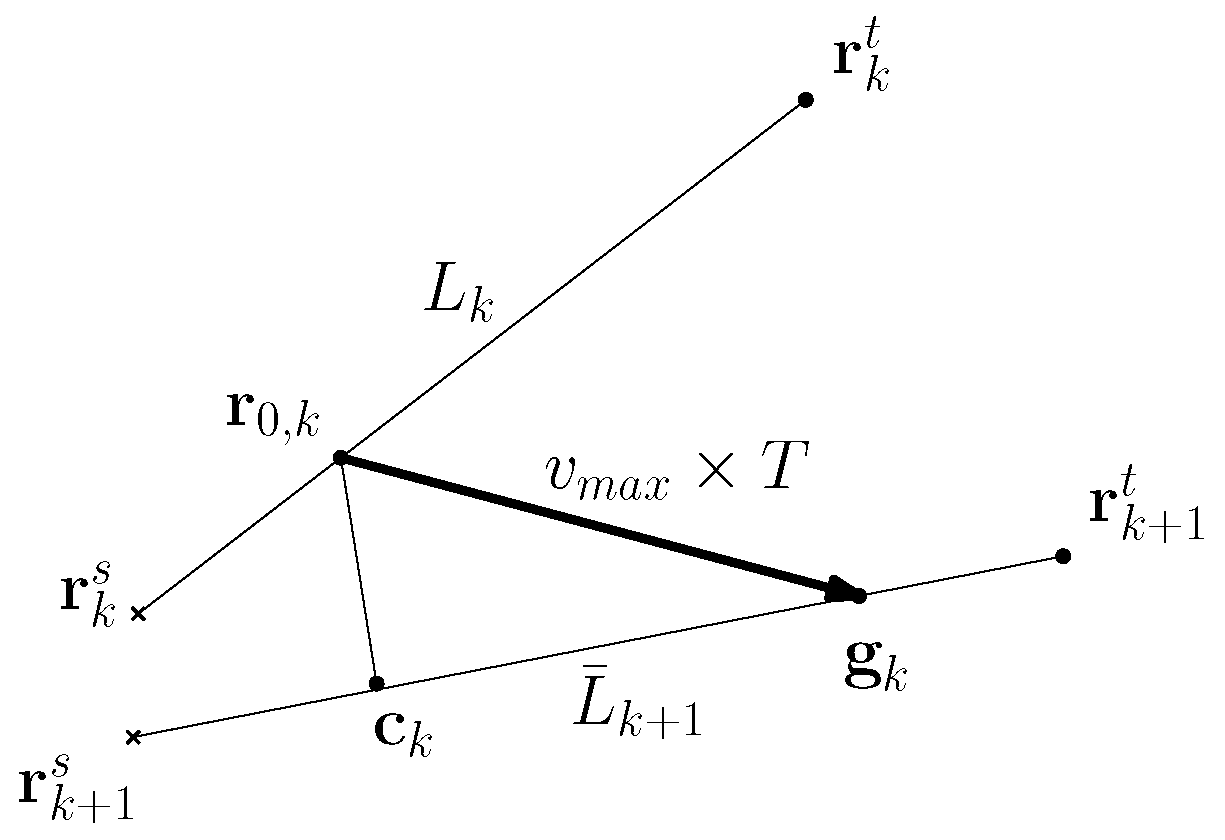
Figure 1 depicts the case where the ship moves as the time index changes from k to $k+1$. The ship positions are indicated by crosses. In this figure, $L_k$, ${\overline{L}}_{k+1}$, and ${\mathbf{c}}_k$ are depicted.

Assumptions

This article assumes that both the ship and a drone’s 3D Cartesian coordinates are measured in real time. Global Positioning Systems (GPSs) and Inertial Measurement Units (IMUs) can be used for this localization.

Furthermore, the ship can measure the target’s 3D Cartesian coordinates at every sample-index. Position measurements can be provided by various sensors, such as radar sensors or laser sensors. Therefore, the ship at sample-index k can derive $L_k$.

Furthermore, based on the target’s recent trajectory, the ship at sample-index k can predict ${\mathbf{r}}_{k+1}^t$, the target’s 3D Cartesian coordinates, after one sample-index in the future. Section 5.1 shows how to predict the target’s 3D Cartesian coordinates after one sample-index in the future.

The ship can also predict ${\mathbf{r}}_{k+1}^s$, the ship’s 3D Cartesian coordinates, after one sample-index in the future. This is feasible because the ship has GPS and IMU. Therefore, the ship can predict ${\overline{L}}_{k+1}$, which crosses both ${\mathbf{r}}_{k+1}^t$ and ${\mathbf{r}}_{k+1}^s$.

It is desirable that as the target is caught, it is sufficiently far from the ship. Otherwise, the ship may be partially caught by the debris of the target. Let $\beta >0$ define the safety distance. The safety distance is set by the operator of the drones. As the target is caught, it is desirable that its distance from the ship is bigger than the safety distance $\beta$. This way, we can assure the safety of the ship.

5. Multi-Drone Guidance Law

We consider a high-speed target whose goal is to hit a ship. The target heads towards its goal (ship) at least in the terminal phase. Otherwise, it is impossible to make a target hit the ship.

Therefore, we let multiple drones form a planar grid formation, whose center lies on the line segment connecting the target and the ship. Moreover, the planar grid formation is generated to be perpendicular to the line segment connecting the target and the formation center. The grid formation can be considered as a “net” structure for capturing the incoming target. By maximizing the grid formation size, we can increase the capture rate, even when there exists error in the prediction of the target’s position. Since the target is guided to hit its goal (the ship), the drones can effectively block the target using this grid formation.

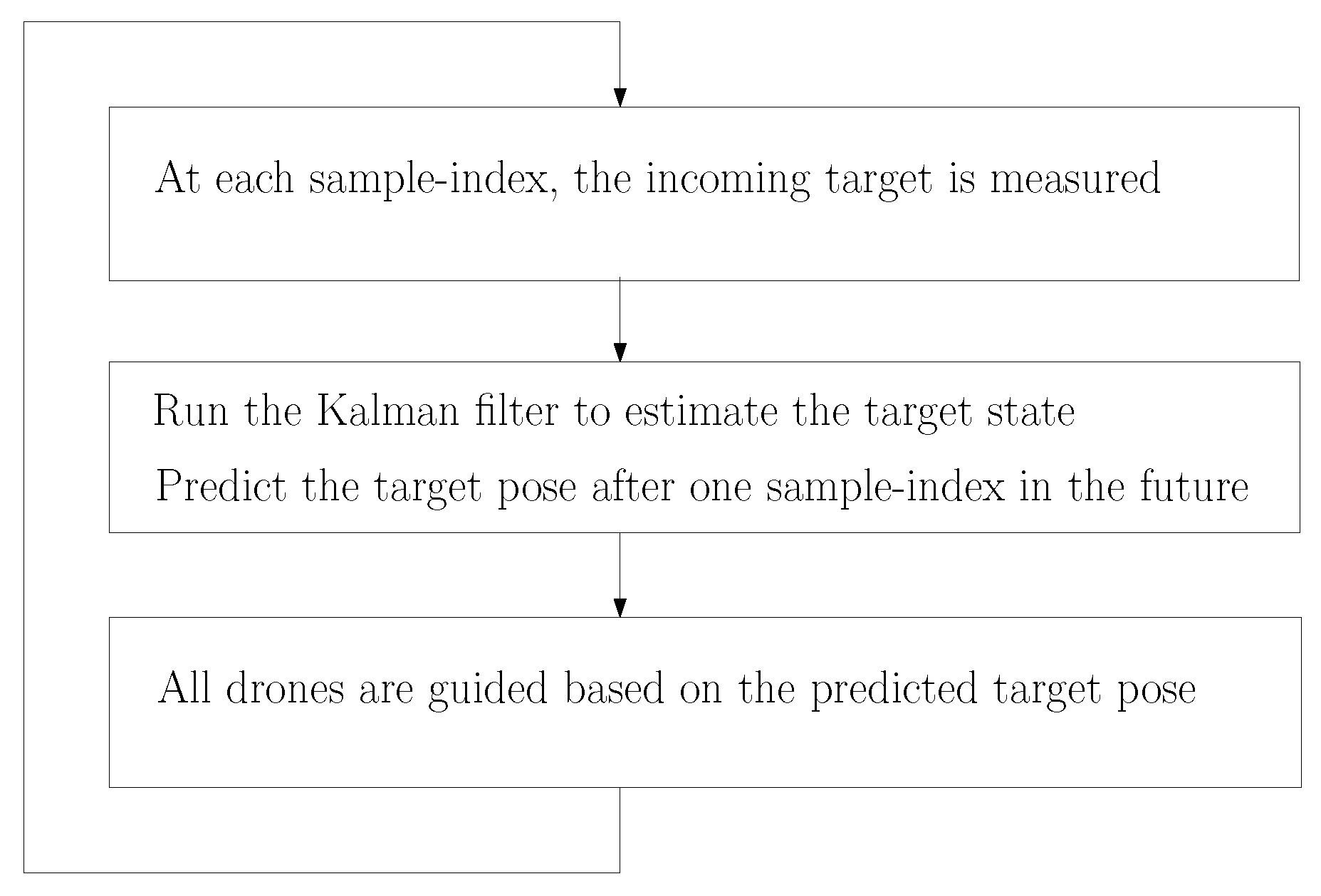
The proposed multi-drone guidance law is summarized as follows. At every sample-index, the ship measures the 3D Cartesian coordinates of the incoming target. Thereafter, we run the Kalman filter to predict the target’s 3D Cartesian coordinates after one sample-index in the future. See Section 5.1 for the prediction of the target’s position after one sample-index.

Based on the predicted target pose, the virtual agent is guided to remain in the lineState. See Section 5.2 for the guidance law of the virtual agent. In addition, each drone is guided to generate a grid formation centered at the virtual agent. See Section 5.3 for the guidance law of a drone. Figure 2 shows the block diagram of the proposed multi-drone guidance law.

5.1. Prediction of the Target’s Position after One Sample-Index

The ship can measure the target’s 3D Cartesian coordinates at every sample-index. To track a target with variable velocity, we present how to predict the target one sample-index forward in time. In order to track a maneuvering target, we applied target-tracking filters to [4].

In the inertial reference frame, let $[x_k^t,y_k^t,z_k^t]$ indicate the vector presenting the 3D coordinates of the target at sample-index k. In addition, ${[{\dot{x}}_k^t,{\dot{y}}_k^t,{\dot{z}}_k^t]}^T$ denotes the vector presenting the target velocity at sample-index k. Furthermore, ${[{\ddot{x}}_k^t,{\ddot{y}}_k^t,{\ddot{z}}_k^t]}^T$ defines the vector presenting the target acceleration at sample-index k. Let ${\mathbf{X}}_k={[x_k^t,{\dot{x}}_k^t,{\ddot{x}}_k^t,y_k^t,{\dot{y}}_k^t,{\ddot{y}}_k^t,z_k^t,{\dot{z}}_k^t,{\ddot{z}}_k^t]}^T$ define the vector presenting the target state. Based on [4], the target’s process model is set as

$$\begin{array}{c}\hfill {\mathbf{X}}_{k+1}=\mathbf{F}\ast {\mathbf{X}}_k+{\mathbf{w}}_k,\end{array}$$

(7)

where ${\mathbf{w}}_k$ is the process noise with following properties: ${\mathbf{w}}_k\sim \mathcal{N}(\mathbf{0},\mathbf{Q})$. Here, $\mathcal{N}(\mathbf{0},\alpha )$ denotes a Gaussian distribution with a mean of $\mathbf{0}$ and a covariance matrix $\alpha$. Furthermore, $\mathbf{F}$ in Equation (7) is

$$\begin{array}{c}\hfill \mathbf{F}=\left(\begin{array}{ccc}{\mathbf{M}}_F& 0& 0\\ 0& {\mathbf{M}}_F& 0\\ 0& 0& {\mathbf{M}}_F\end{array}\right),\end{array}$$

(8)

where we use

$$\begin{array}{c}\hfill {\mathbf{M}}_F=\left(\begin{array}{ccc}1,& T,& \frac{a\ast T-1+e^{-a\ast T}}{a^2}\\ 0,& 1,& \frac{1+e^{-a\ast T}}{a^2}\\ 0,& 0,& e^{-a\ast T}\end{array}\right).\end{array}$$

(9)

In ${\mathbf{w}}_k$, $\mathbf{Q}$ is set as

$$\begin{array}{c}\hfill \mathbf{Q}=2\ast a\ast {\sigma }_m^2\ast \left(\begin{array}{ccc}{\mathbf{M}}_Q& 0& 0\\ 0& {\mathbf{M}}_Q& 0\\ 0& 0& {\mathbf{M}}_Q\end{array}\right),\end{array}$$

(10)

where

$$\begin{array}{c}\hfill {\mathbf{M}}_Q=\left(\begin{array}{ccc}{T}^5/20,& T^4/8,& T^3/6\\ T^4/8,& T^3/6,& T^2/2\\ T^3/6,& T^2/2,& T\end{array}\right).\end{array}$$

(11)

a and ${\sigma }_m$ in Equation (10) are tuning parameters for tracking a maneuvering target. Detailed derivations of Equation (7) appear in [4].

At every sample-index k, the ship measures the target’s 3D position, say ${\mathbf{m}}_k$. See the first block of Figure 2. The target measurement model is

$$\begin{array}{c}\hfill {\mathbf{m}}_k=\mathbf{H}\ast {\mathbf{X}}_k+{\mathbf{v}}_k\end{array}$$

(12)

where $\mathbf{H}$ is

$$\begin{array}{c}\hfill \mathbf{H}=\left(\begin{array}{ccccccccc}1& 0& 0& 0& 0& 0& 0& 0& 0\\ 0& 0& 0& 1& 0& 0& 0& 0& 0\\ 0& 0& 0& 0& 0& 0& 1& 0& 0\end{array}\right).\end{array}$$

(13)

Furthermore, ${\mathbf{v}}_k$ is the measurement noise, such that ${\mathbf{v}}_k\sim \mathcal{N}(\mathbf{0},{\mathbf{R}}_k)$. We assume that ${\mathbf{R}}_k$ is known a priori.

The Kalman filter (KF) [47] is applied to obtain the estimate vector and its covariance at every sample-index. The KF is composed of the prediction step and the measurement update step. In the KF, the prediction step uses Equation (7), and the measurement update step uses Equation (12).

Let ${\widehat{\mathbf{X}}}_{k|k}$ define the estimation of ${\mathbf{X}}_k$ derived using all measurements up to sample-index k. Let ${\mathbf{P}}_{k|k}$ define the error covariance matrix of ${\widehat{\mathbf{X}}}_{k|k}$.

In the prediction step of the KF, we derive the predicted state vector as

$$\begin{array}{c}\hfill {\widehat{\mathbf{X}}}_{k+1|k}=\mathbf{F}\ast {\widehat{\mathbf{X}}}_{k|k},\end{array}$$

(14)

where Equation (7) is used. Utilizing Equations (7) and (10), the covariance matrix is predicted as

$${\mathbf{P}}_{k+1|k}=\mathbf{F}\ast {\mathbf{P}}_{k|k}\ast {\mathbf{F}}^T+\mathbf{Q}.$$

(15)

The measurement update step is

$${\widehat{\mathbf{X}}}_{k+1|k+1}={\widehat{\mathbf{X}}}_{k+1|k}+{\mathbf{W}}_k\ast ({\mathbf{m}}_k-\mathbf{H}\ast {\widehat{\mathbf{X}}}_{k+1|k}),$$

(16)

where

$${\mathbf{W}}_k={\mathbf{P}}_{k+1|k}\ast {\mathbf{H}}^T\ast {\mathbf{S}}^{-1}.$$

(17)

Here, we use

$$\begin{array}{c}\hfill \mathbf{S}=\mathbf{H}{\mathbf{P}}_{k+1|k}{\mathbf{H}}^T+{\mathbf{R}}_k.\end{array}$$

(18)

In addition, the covariance matrix is updated using

$${\mathbf{P}}_{k+1|k+1}={\mathbf{P}}_{k+1|k}-{\mathbf{W}}_k\ast \mathbf{S}\ast {\mathbf{W}}_k^T.$$

(19)

The ship at sample-index k predicts the target state after one sample-index forward in time using Equation (14). Let ${\widehat{\mathbf{r}}}_{k+1}^t$ denote the target position at sample-index $k+1$, which is predicted using all measurements up to sample-index k. Using Equation (14), ${\widehat{\mathbf{r}}}_{k+1}^t$ is predicted as

$$\begin{array}{c}\hfill {\widehat{\mathbf{r}}}_{k+1}^t=\mathbf{H}\ast {\widehat{\mathbf{X}}}_{k+1|k}.\end{array}$$

(20)

Here, recall that $\mathbf{H}$ was defined in Equation (13).

We acknowledge that the prediction of the target’s position may not be accurate due to the target’s elusive maneuvers or measurement noise. This is the motivation for using a formation of drones instead of a single drone.

In our paper, a formation of drones is used instead of a single drone in order to increase the capture rate. Since we use a drone formation, we can increase the capture rate even when the target prediction is erroneous. Through MATLAB simulations, the effectiveness of our formation-based guidance law is verified by comparing it with other state-of-the-art guidance controls.

5.2. Guidance Law of the Virtual Agent

Using the predicted 3D coordinates of the target, the virtual agent is guided to remain in the lineState. At every sample-index k, the virtual agent is guided to head towards the guidance point ${\mathbf{g}}_k$, which is defined as follows:

1. Suppose that $\parallel {\mathbf{r}}_k^s-{\mathbf{r}}_{0,k}\parallel <\beta$. This implies that the ship needs to expel the virtual agent away from the ship. Moreover, suppose that

$$\begin{array}{c}\hfill \parallel {\mathbf{r}}_{0,k}-{\mathbf{c}}_k\parallel \le v_{max}\ast T\end{array}$$

(21)

holds. Then, we set the guidance point as

$$\begin{array}{ccc}\hfill {\mathbf{g}}_k& =& {\mathbf{c}}_k+\frac{{\mathbf{r}}_{k+1}^t-{\mathbf{c}}_k}{\parallel {\mathbf{r}}_{k+1}^t-{\mathbf{c}}_k\parallel }\ast {\delta }_k.\hfill \end{array}$$

(22)

Here, ${\delta }_k>0$ is defined as

$$\begin{array}{c}\hfill {\delta }_k=\sqrt{{(v_{max}\ast T)}^2-{(\parallel {\mathbf{r}}_{0,k}-{\mathbf{c}}_k\parallel )}^2}.\end{array}$$

(23)

This implies that $\parallel {\mathbf{g}}_k-{\mathbf{r}}_{0,k}\parallel$ is $v_{max}\ast T$. See Figure 1 for an illustration of this case.

2. Otherwise, we set the guidance point as

$$\begin{array}{ccc}\hfill {\mathbf{g}}_k& =& {\mathbf{c}}_k.\hfill \end{array}$$

(24)

At every sample-index k, the virtual agent moves to reach ${\mathbf{g}}_k$ if possible. Suppose that $\parallel {\mathbf{r}}_k^s-{\mathbf{r}}_{0,k}\parallel <\beta$. Furthermore, suppose that Equation (21) holds, as depicted in Figure 1. Consider a sphere centered at ${\mathbf{r}}_{0,k}$, whose radius is $v_{max}\ast T$. Using Equation (21), ${\overline{L}}_{k+1}$ meets this sphere at two points. Between these two points, ${\mathbf{g}}_k$ is the point that is closer to ${\mathbf{r}}_{k+1}^t$. In this way, the virtual agent can approach the target while staying on the line segment that connects the target and the ship.

The direction command ${\mathbf{u}}_{0,k}$ is selected to make the virtual agent move towards ${\mathbf{g}}_k$ at sample-index $k+1$. At every sample-index k, the direction command is set as follows. At every sample-index k, the virtual agent sets the new direction command ${\mathbf{u}}_{0,k}$ as

$$\begin{array}{c}\hfill {\mathbf{u}}_{0,k}=\frac{{\mathbf{g}}_k-{\mathbf{r}}_{0,k}}{\parallel {\mathbf{g}}_k-{\mathbf{r}}_{0,k}\parallel }.\end{array}$$

(25)

Note that the direction command is a unit vector.

In addition, the speed command at sample-index k is set as follows. At every sample-index k, the virtual agent sets the new speed command $v_{0,k}$ as

$$\begin{array}{c}\hfill v_{0,k}=min(\frac{\parallel {\mathbf{g}}_k-{\mathbf{r}}_{0,k}\parallel }{T},v_{max}).\end{array}$$

(26)

This implies that the virtual agent moves with the maximum speed $v_{max}$ when it is too far from the guidance point ${\mathbf{g}}_k$.

Consider the situation in which $\parallel {\mathbf{r}}_{0,k}-{\mathbf{r}}_{k+1}^t\parallel <v_{max}\ast T$ holds. In this situation, the virtual agent heads towards ${\mathbf{r}}_{k+1}^t$ directly while not using the direction command ${\mathbf{u}}_{0,k}=\frac{{\mathbf{g}}_k-{\mathbf{r}}_{0,k}}{\parallel {\mathbf{g}}_k-{\mathbf{r}}_{0,k}\parallel }$. In this way, the target is caught at sample-index $k+1$.

According to the definitions of the guidance point ${\mathbf{g}}_k$ (see Equations (22) and (24)), ${\mathbf{g}}_k$ lies on $l({\mathbf{r}}_{k+1}^t,{\mathbf{r}}_{k+1}^s)$.

In the case where $\frac{\parallel {\mathbf{g}}_k-{\mathbf{r}}_{0,k}\parallel }{T}\le v_{max}$, the heading command (Equation (25)) and speed command (Equation (26)) lead to

$$\begin{array}{c}\hfill {\mathbf{r}}_{0,k+1}={\mathbf{g}}_k.\end{array}$$

(27)

We thus have the following theorem.

Theorem 1. 

Suppose that $\frac{\parallel {\mathbf{c}}_k-{\mathbf{r}}_{0,k}\parallel }{T}\le v_{max}$. The heading command (Equation (25)) and speed command (Equation (26)) make ${\mathbf{r}}_{0,k+1}$ exist on $l({\mathbf{r}}_{k+1}^t,{\mathbf{r}}_{k+1}^s)$.

Theorem 1 implies that in the case where $\frac{\parallel {\mathbf{c}}_k-{\mathbf{r}}_{0,k}\parallel }{T}\le v_{max}$, the virtual agent position ${\mathbf{r}}_{0,k+1}$ is on the line segment $l({\mathbf{r}}_{k+1}^t,{\mathbf{r}}_{k+1}^s)$. Since the target’s goal is reaching the ship, the target must be hit by the virtual agent eventually.

$L_k$ and ${\overline{L}}_{k+1}$ Meet at a Point

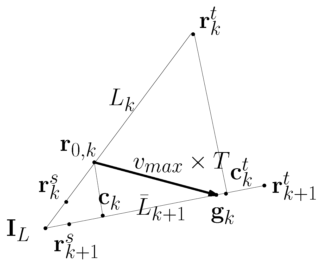
Next, we consider a special case where $L_k$ and ${\overline{L}}_{k+1}$ meet at a point. Here, recall that ${\overline{L}}_{k+1}$ denotes the infinite line crossing both ${\mathbf{r}}_{k+1}^s$ and ${\mathbf{r}}_{k+1}^t$. In the inertial reference frame, let ${\mathbf{I}}_L$ denote the 3D coordinates of the intersection between $L_k$ and ${\overline{L}}_{k+1}$. For instance, if the ship is static, then $L_k$ and ${\overline{L}}_{k+1}$ meet at the ship position ${\mathbf{r}}_k^s={\mathbf{r}}_{k+1}^s$.

Suppose that ${\mathbf{r}}_{0,k}$ lies on $l({\mathbf{r}}_k^t,{\mathbf{r}}_k^s)$. Let ${\mathbf{c}}_k^t$ denote the point on ${\overline{L}}_{k+1}$, which is the closest to ${\mathbf{r}}_k^t$. Let $l_k=\parallel {\mathbf{c}}_k-{\mathbf{r}}_{0,k}\parallel$ for convenience.

Figure 3 depicts the case where $L_k$ and ${\overline{L}}_{k+1}$ meet at ${\mathbf{I}}_L$. Using the geometry in this figure, we have

$$\begin{array}{c}\hfill \parallel {\mathbf{c}}_k^t-{\mathbf{r}}_k^t\parallel =\frac{l_k\ast \parallel {\mathbf{I}}_L-{\mathbf{r}}_k^t\parallel }{\parallel {\mathbf{I}}_L-{\mathbf{r}}_{0,k}\parallel }.\end{array}$$

(28)

Since the target speed is $v_k^t$, we have

$$\begin{array}{c}\hfill v_k^t\ast T\ge \parallel {\mathbf{c}}_k^t-{\mathbf{r}}_k^t\parallel .\end{array}$$

(29)

Using Equations (28) and (29), we have

$$\begin{array}{c}\hfill \frac{v_k^t\ast T\ast \parallel {\mathbf{I}}_L-{\mathbf{r}}_{0,k}\parallel }{\parallel {\mathbf{I}}_L-{\mathbf{r}}_k^t\parallel }\ge l_k.\end{array}$$

(30)

Suppose that the drone’s maximum speed $v_{max}$ satisfies

$$\begin{array}{c}\hfill v_{max}>\frac{v_k^t\ast \parallel {\mathbf{I}}_L-{\mathbf{r}}_{0,k}\parallel }{\parallel {\mathbf{I}}_L-{\mathbf{r}}_k^t\parallel }.\end{array}$$

(31)

The next theorem addresses the condition for remaining in the lineState at every sample-index.

Theorem 2. 

Suppose that $L_k$ and ${\overline{L}}_{k+1}$ meet at a point, say ${\mathbf{I}}_L$. Suppose that ${\mathbf{r}}_{0,k}$ lies on $l({\mathbf{r}}_k^t,{\mathbf{r}}_k^s)$. The target speed is $v_k^t$. If the drone’s maximum speed satisfies Equation (31), then ${\mathbf{r}}_{0,k+1}$ lies on $l({\mathbf{r}}_{k+1}^t,{\mathbf{r}}_{k+1}^s)$.

Proof. 

Suppose the drone’s maximum speed satisfies Equation (31). Then, Equations (30) and (31) lead to

$$\begin{array}{c}\hfill v_{max}\ast T>l_k.\end{array}$$

(32)

This implies that Equation (21) is met. In the case where Equation (21) is met, Theorem 1 makes ${\mathbf{r}}_{0,k+1}$ exist on $l({\mathbf{r}}_{k+1}^t,{\mathbf{r}}_{k+1}^s)$. The proof is complete. □

In practice, the ship moves much slower than the target. Thus, the ship position is close to ${\mathbf{I}}_L$, as plotted in Figure 3. Consider the case where the virtual agent is sufficiently close to the ship. In this case, $\parallel {\mathbf{I}}_L-{\mathbf{r}}_{0,k}\parallel$ is small to satisfy Equation (31). Then, using Corollary 2, ${\mathbf{r}}_{0,k+1}$ lies on $l({\mathbf{r}}_{k+1}^t,{\mathbf{r}}_{k+1}^s)$. Thus, the virtual agent remains in the lineState at sample-index $k+1$.

In the case where the virtual agent stays in the lineState at all times, the target cannot reach the ship without being captured by the virtual agent. In order to stay in the lineState at each sample-index, it is desirable that the virtual agent does not become too far from the ship.

In the case where $\parallel {\mathbf{r}}_k^s-{\mathbf{r}}_{0,k}\parallel \ge \beta$ is met, the guidance point is set using Equation (24) instead of Equation (22). In this way, drones stay close to the ship while staying in the lineState at all times.

Note that Equation (31) can be satisfied even when $v_{max}<v_k^t$. This implies that even slow drones can capture a fast target when the drones stay close to the ship while staying in the lineState at all times.

5.3. Guidance Law of Every Drone

We let multiple drones form a planar grid formation, such that the formation is perpendicular to the line segment connecting the target and the formation center. The grid formation can be considered a “net” structure for capturing the incoming target. By maximizing the grid formation size, we can increase the capture rate, even when there exists error in the prediction of the target’s position. Since the target is guided to hit its goal (ship), the drones can effectively block the target using this grid formation.

We next handle the guidance law of a drone for the generation of the grid formation. At sample-index k, let grid formation denote a planar formation composed of $G\times G$ cells, each with side length $s_k$. The grid formation is centered at the virtual agent, and we adjust the grid formation so that it is normal to $l({\mathbf{r}}_k^t,{\mathbf{r}}_{0,k})$ at each sample-index k. We change the pitch and yaw of the virtual agent, but we do not change the roll of the virtual agent. Thus, the grid formation does not roll either.

Let ${\mathbf{r}}_k^R={\mathbf{r}}_k^t-{\mathbf{r}}_{0,k}$ denote the relative position of the target with respect to the virtual agent at sample-index k. At each sample-index k, the planar grid formation is oriented, such that the formation plane is perpendicular to ${\mathbf{r}}_k^R$.

For $i\in \{0,1,2,\dots ,G-1\}$ and $j\in \{0,1,\dots ,G-1\}$, let $n[i,j]$ be defined as

$$\begin{array}{c}\hfill n[i,j]=1+i+G\ast j.\end{array}$$

(33)

Since $i\in \{0,1,2,\dots ,G-1\}$ and $j\in \{0,1,2,\dots ,G-1\}$, we have

$$\begin{array}{c}\hfill n[i,j]\in \{1,2,\dots ,M=G^2\}.\end{array}$$

(34)

Here, Equation (4) is used. Using Equations (33) and (34), the drone index $n\in \{1,2,\dots ,M=G^2\}$ has its associated $n[i,j]$.

For $i\in \{0,1,2,\dots ,G-1\}$ and $j\in \{0,1,\dots ,G-1\}$, let

$$\begin{array}{c}\hfill {\mathbf{w}}_{n[i,j],k}^B={(0,-\frac{s_k\ast G}{2}+i\ast s_k,-\frac{s_k\ast G}{2}+j\ast s_k)}^T\end{array}$$

(35)

denote the n-th drone’s waypoint in the body-fixed frame at sample-index k. See that these $G\times G$ waypoints are generated on the $yz$ plane in the body-fixed frame. From now on, n denotes $n[i,j]$ for notation simplicity.

In the case where we set $G=1$, we use only one drone. In this case, the grid formation cannot be generated. If we use only one drone, then the drone’s waypoint in the body-fixed frame is set as

$$\begin{array}{c}\hfill {\mathbf{w}}_{1,k}^B={(0,0,0)}^T,\end{array}$$

(36)

instead of Equation (35). Equation (36) is used to make the single drone move towards the virtual agent. In other words, the waypoint of the drone is set as the virtual agent.

At sample-index 0, all drones are located inside the grid cell of the ship. At sample-index 0, the planar grid formation’s orientation (normal vector) is represented as initial yaw ${\psi }_0=0$ and initial pitch ${\theta }_0=\pi /2$, respectively. Under Equation (3), the n-th drone’s initial position is located at ${\mathbf{w}}_{n,0}$, which is given as

$$\begin{array}{c}\hfill {\mathbf{w}}_{n,0}={\mathbf{M}}_R(0,\pi /2)\ast {\mathbf{w}}_{n,0}^B.\end{array}$$

(37)

Equation (37) implies that all drones are initially located to form the grid formation with side length $s_0$.

Once the drones are launched from the ship, the planar grid formation at each sample-index k is oriented, such that it becomes perpendicular to ${\mathbf{r}}_k^R={\mathbf{r}}_k^t-{\mathbf{r}}_{0,k}$. The unit vector associated with ${\mathbf{r}}_k^R$ is

$$\begin{array}{c}\hfill {\mathbf{u}}^R={({\mathbf{u}}^R\left(1\right),{\mathbf{u}}^R\left(2\right),{\mathbf{u}}^R\left(3\right))}^T,\end{array}$$

(38)

where ${\mathbf{u}}^R=\frac{{\mathbf{r}}_k^R}{\parallel {\mathbf{r}}_k^R\parallel }$.

At each sample-index k, the planar grid formation’s orientation (normal vector) is represented as ${\psi }_k$ and ${\theta }_k$, respectively. Since the virtual agent does not rotate, the formation’s orientation does not include rolling motions. Under Equation (3), the n-th drone’s waypoint in the inertial frame is

$$\begin{array}{c}\hfill {\mathbf{w}}_{n,k}={\mathbf{r}}_{0,k}+{\mathbf{M}}_R({\psi }_k,{\theta }_k)\ast {\mathbf{w}}_{n,k}^B.\end{array}$$

(39)

The axis of the grid formation is oriented towards the target ${\mathbf{r}}_k^t$ since ${\mathbf{u}}^R=\frac{{\mathbf{r}}_k^R}{\parallel {\mathbf{r}}_k^R\parallel }$, where ${\mathbf{r}}_k^R={\mathbf{r}}_k^t-{\mathbf{r}}_{0,k}$. In other words, the planar grid formation is oriented such that it is perpendicular to ${\mathbf{r}}_k^R$.

We next calculate the planar grid formation’s orientation (normal vector), ${\psi }_k$, and ${\theta }_k$ in Equation (39), associated with ${\mathbf{u}}^R$ in Equation (38). We apply ${\mathbf{u}}^R\left(1\right)=c\left({\psi }_k\right)\ast c\left({\theta }_k\right)$, ${\mathbf{u}}^R\left(2\right)=s\left({\psi }_k\right)\ast c\left({\theta }_k\right)$, and ${\mathbf{u}}^R\left(3\right)=-s\left({\theta }_k\right)$. Here, ${\mathbf{u}}^R\left(j\right)$ indicates the j-th element of ${\mathbf{u}}^R$.

Under Equation (38), we obtain

$$\begin{array}{c}\hfill {\theta }_k=atan2(-{\mathbf{u}}^R\left(3\right),\sqrt{{\mathbf{u}}^R{\left(1\right)}^2+{\mathbf{u}}^R{\left(2\right)}^2}).\end{array}$$

(40)

Under Equation (38), we derive ${\psi }_k$ as follows. If $c\left({\theta }_k\right)\ge 0$, then we use

$$\begin{array}{c}\hfill {\psi }_k=atan2({\mathbf{u}}^R\left(2\right),{\mathbf{u}}^R\left(1\right)).\end{array}$$

(41)

If $c\left({\theta }_k\right)<0$, then we use

$$\begin{array}{c}\hfill {\psi }_k=atan2(-{\mathbf{u}}^R\left(2\right),-{\mathbf{u}}^R\left(1\right)).\end{array}$$

(42)

Recall that ${\mathbf{w}}_{n,k}$ defines the waypoint assigned to the n-th drone at sample-index k. The heading command of the n-th drone is set towards ${\mathbf{w}}_{n,k}$ at every sample-index k. The heading vector ${\mathbf{u}}_{n,k}$ from Equation (5) is set as follows.

$$\begin{array}{c}\hfill {\mathbf{u}}_{n,k}=\frac{{\mathbf{w}}_{n,k}-{\mathbf{r}}_{n,k}}{\parallel {\mathbf{w}}_{n,k}-{\mathbf{r}}_{n,k}\parallel }.\end{array}$$

(43)

At every sample-index k, the n-th drone sets its speed command $v_{n,k}$ from Equation (5) as

$$\begin{array}{c}\hfill v_{n,k}=min(\frac{\parallel {\mathbf{w}}_{n,k}-{\mathbf{r}}_{n,k}\parallel }{T},v_{max}).\end{array}$$

(44)

The control commands, Equations (43) and (44), are used to satisfy

$$\begin{array}{c}\hfill {\mathbf{r}}_{n,k+1}={\mathbf{w}}_{n,k},\end{array}$$

(45)

if possible. Once Equation (45) is met for all $n\in \{1,2,\dots ,M\}$, then all drones form a grid formation at sample-index $k+1$.

Consider the case where $\parallel {\mathbf{r}}_{n,k}-{\mathbf{w}}_{n,k}\parallel <v_{max}\ast T$ at every sample-index k. In this case, Equation (45) is met at every sample-index k.

At sample-index 0, all drones are located inside the ship. At sample-index 0, all drones form the initial grid formation, as presented in Equation (37). Note that each drone is assigned to a waypoint that is in the body-fixed frame of the virtual agent. See Equation (39) for waypoint assignments.

Moreover, [48] can be used to assign a drone to each waypoint, such that the makespan (time for all robots to reach their waypoints) is minimized while also preventing collisions among drones. The authors of [48] mentioned that their assignment algorithm scales well, such that it can compute the mapping for 1000 robots in less than half a second.

In the worst case, there may be a case where a drone meets another drone while moving toward its assigned waypoint. This case can happen due to localization errors or environment disturbance, such as wind. The drone then uses reactive collision avoidance controls, such as [49,50,51,52], to avoid an abrupt collision with another drone. Under reactive collision avoidance controls, the drone can change its speed and heading to avoid a sudden collision. We acknowledge that a drone may not reach its waypoint, as it performs evasive maneuvers to avoid a sudden collision with another drone. For instance, suppose that a drone slows downs to avoid a sudden collision at sample-index k. At the next sample-index $k+1$, the drone needs to speed up to reach its new waypoint at sample-index $k+1$.

Control of the Side Length in the Grid Formation

Considering the uncertainty in the target position, it is desirable to make the formation cover as large of an area as possible. However, in the case where the formation is too sparse, the target can get through the formation without being captured by a drone. Furthermore, in the case where the formation is too dense, a large number of drones must be used to cover a large area.

Recall that $s_k$ denotes the side length at sample-index k. Initially, all drones are stored in the grid cells of the ship, such that $s_0=1$ meters in Equation (37).

Let $s^u$ denote the upper bound for the side length. In order to capture a target, the side length is increased gradually using

$$\begin{array}{c}\hfill s_k=\eta \ast s_{k-1}+(1-\eta )\ast s^u.\end{array}$$

(46)

Here, $0<\eta <1$ is a positive constant. $\eta$ is a tuning parameter indicating the sensitivity for the radius update. In MATLAB simulations, $\eta =0.9$ is used. As time elapses, $s_k$ monotonically increases to $s^u$. This implies that the formation size increases as time elapses.

Recall that a target is captured when the relative distance between the target and a drone is less than $\Delta$. In the simulation section, $\Delta =10$ m is used. If $s^u\le \Delta$, then the target cannot get through the grid “net” generated by the drones. Thus, $s^u=\Delta$ is set in our simulations.

6. MATLAB Simulation

This section demonstrates the effectiveness of our multi-agent guidance law through MATLAB simulations. The sample interval is $T=0.5$ s. The safety distance $\beta$ is set as 100 m.

In Equation (12), the measurement noise ${\mathbf{v}}_k$ is generated with ${\mathbf{v}}_k\sim \mathcal{N}(\mathbf{0},{\mathbf{R}}_k)$, where ${\mathbf{R}}_k$ is the identity matrix such that every diagonal element is 1. This implies that the standard deviation of measurement noise is 1 meter.

Considering the process noise, the motion model of the i-th drone ($i\in \{1,2,\dots ,M\}$) is

$$\begin{array}{c}\hfill {\mathbf{r}}_{i,k+1}={\mathbf{r}}_{i,k}+T\ast v_{i,k}\ast {\mathbf{u}}_{i,k}+{\mathbf{n}}_i.\end{array}$$

(47)

Here, ${\mathbf{n}}_i$ indicates the process noise of the i-th drone, such that each term in ${\mathbf{n}}_i$ has a Gaussian distribution with a mean of 0 and a standard deviation of 1 meter. Because Equation (47) contains the process noise term ${\mathbf{n}}_i$, Equation (47) is distinct from Equation (5).

At sample-index 0, the target is at (0, 10,000, 5000) in meters, and the virtual agent is at the origin. The ship is located at (0,0,0) at sample-index 0. Furthermore, the maximum speed of a drone is $v_{max}=20$ meters per second. At every sample-index k, the target’s speed, $v_k^t$, is 200 meters per second. See that the target moves much faster than a drone.

We say that a target is captured when the distance between a drone and the target is less than $\Delta =10$ meters. Moreover, a target is captured at sample-index k when $l({\mathbf{r}}_k^t,{\mathbf{r}}_{k-1}^t)$ crosses the grid formation between sample-index $k-1$ and k. Because $s^u=\Delta$, the target is considered to be captured between sample-index $k-1$ and k.

Furthermore, a simulation ends when the distance between the ship and the target is less than $\Delta$. This implies that the ship is hit by the target.

6.1. Monte-Carlo Simulations

Multiple Monte-Carlo (MC) simulations are needed to prove the effectiveness of the proposed method rigorously since the measurements are noisy. We run $mC=50$ MC simulations while changing generated noise.

At the end of each MC simulation, the target hits the ship or is captured by a drone. We use three metrics ($captureRate$, $endDist$, and $simTime$) to analyze the proposed controls.

Let $captureN$ denote the number of MC simulations where the target is captured by a drone. Considering the analysis of $mC$ MC simulations, $captureRate=\frac{captureN}{mC}$ presents the capture rate (in percents) as we run $mC$ MC simulations. It is desirable that the $captureRate$ is as large as possible.

Let $endDist$ (m) represent the average distance between the ship and all drones’ center position when an MC simulation ends. In the case where a single drone is considered, $endDist$ represents the average distance between the ship and the drone when an MC simulation ends. Large $endDist$ implies that at the end of a simulation, a drone is far from the ship.

Let $simTime$ denote the average time (in seconds) spent until each MC simulation ends. Note that an MC simulation ends when the target hits the ship or is captured by a drone.

6.2. 3D PNG Law

The target applies the PNG laws in [20] to approach the ship as time elapses. We briefly introduce the 3D PNG law in [20]. The rotation vector of the line-of-sight at sample-index k is

$$\begin{array}{c}\hfill {\mathsf{\Omega }}_{st,k}={\mathbf{R}}_{st,k}\ast {\mathbf{V}}_{st,k}/\left(r^2\right),\end{array}$$

(48)

where ${\mathbf{V}}_{st,k}$ is the relative velocity of the ship with respect to the target. Furthermore, ${\mathbf{R}}_{st,k}={\mathbf{r}}_k^s-{\mathbf{r}}_k^t$, and $r=\parallel {\mathbf{R}}_{st,k}\parallel$. The PNG law is set as

$$\begin{array}{c}\hfill {\mathbf{c}}_{png,k}=N_p{\mathbf{V}}_{st,k}\ast {\mathsf{\Omega }}_{st,k},\end{array}$$

(49)

where $N_p=3$ is a constant. The target’s velocity is updated as

$$\begin{array}{c}\hfill {\mathbf{v}}_{k+1}^t={\mathbf{v}}_k^t+T\ast {\mathbf{c}}_{png,k}.\end{array}$$

(50)

Then, the target’s position is updated using

$$\begin{array}{c}\hfill {\mathbf{r}}_{k+1}^t={\mathbf{r}}_k^t+T\ast v_k^t\frac{{\mathbf{v}}_k^t}{\parallel {\mathbf{v}}_k^t\parallel }.\end{array}$$

(51)

6.3. Scenario 1

In this scenario, the ship moves at a velocity of (−5,0,0) in m/s.

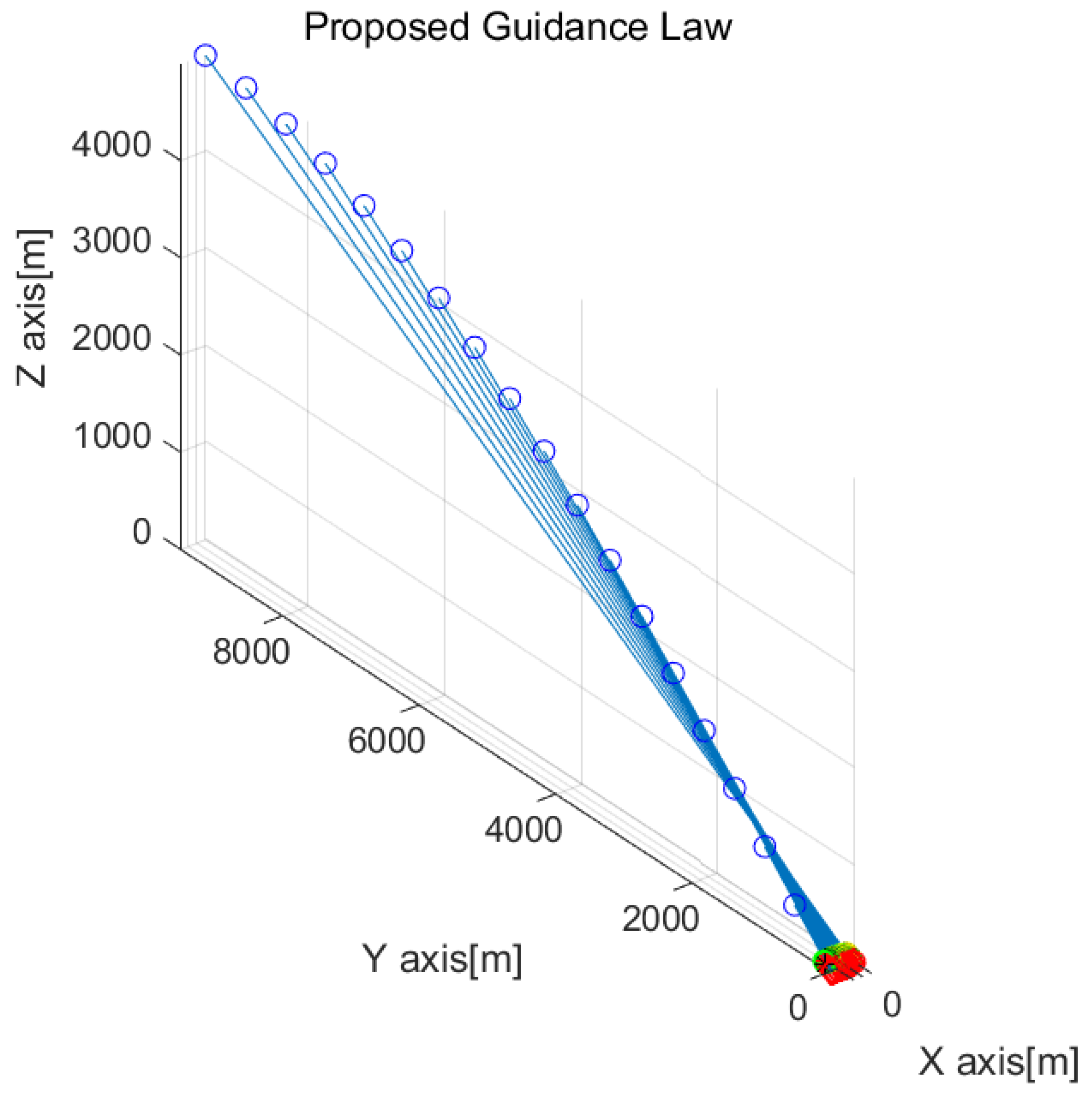
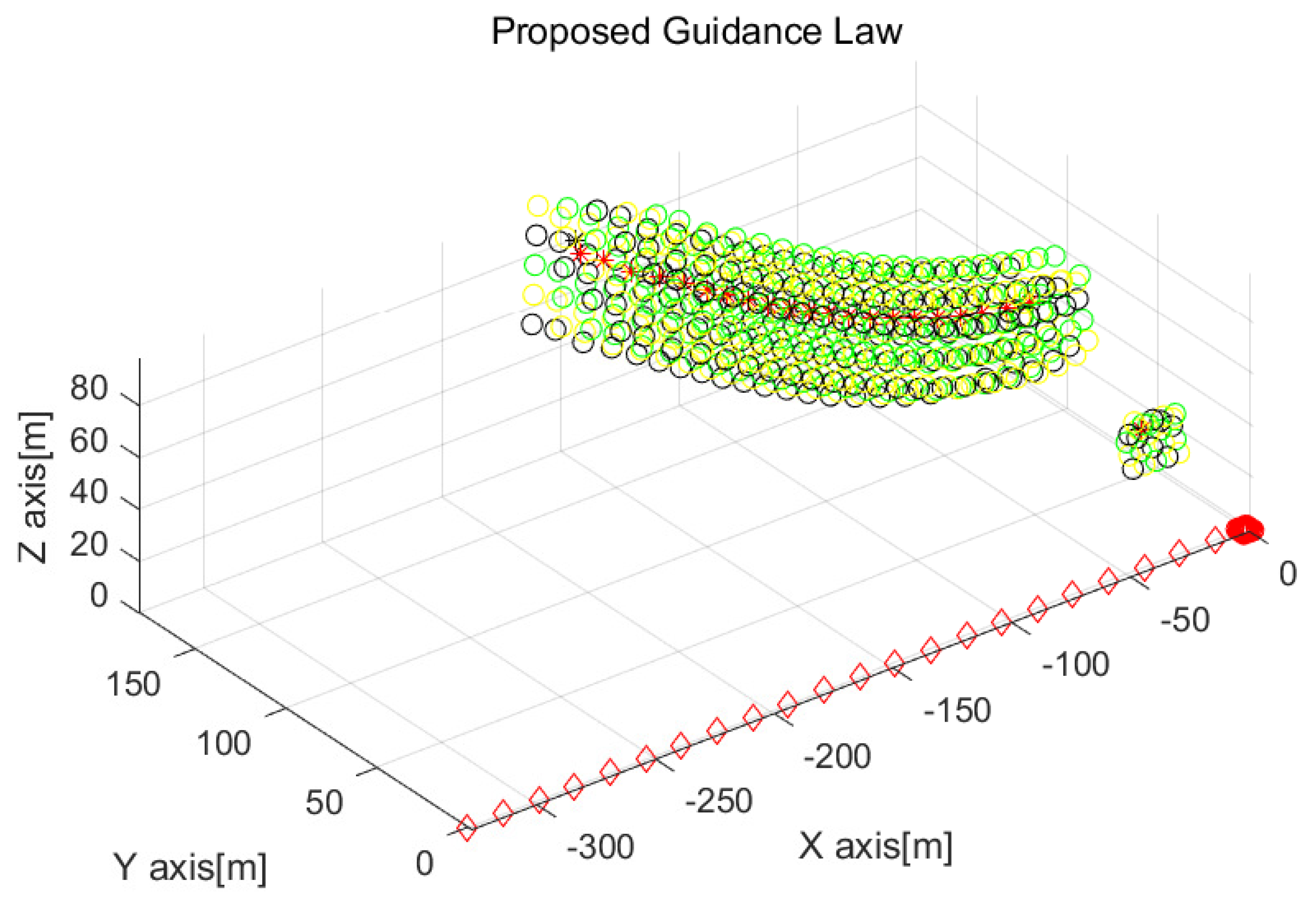
We set $G=3$ in Equation (4). This implies that we use $M=G^2=9$ drones in total. Figure 4 shows the result of one MC simulation using nine drones. In Figure 4, the target’s position at every 3 s is marked as blue circles. The position of every drone at every 3 s is depicted as circles with distinct colors. A red asterisk depicts the position of the virtual agent at every 3 s. The position of the ship at every 3 s is indicated by red diamonds.

Figure 5 is the enlarged figure of Figure 4. The position of every drone at every 3 s is depicted as circles with distinct colors. The drones generate a grid formation for protection against the incoming target.

Considering the scenario in Figure 5, Figure 6 removes the plots for the target’s positions in order to see the drones’ maneuvers clearly. The position of every drone at every 3 s is depicted as circles with distinct colors. A red asterisk depicts the position of the virtual agent at every 3 s. The position of the ship at every 3 s is indicated by red diamonds. A black asterisk presents the target’s position when the target is hit by a drone.

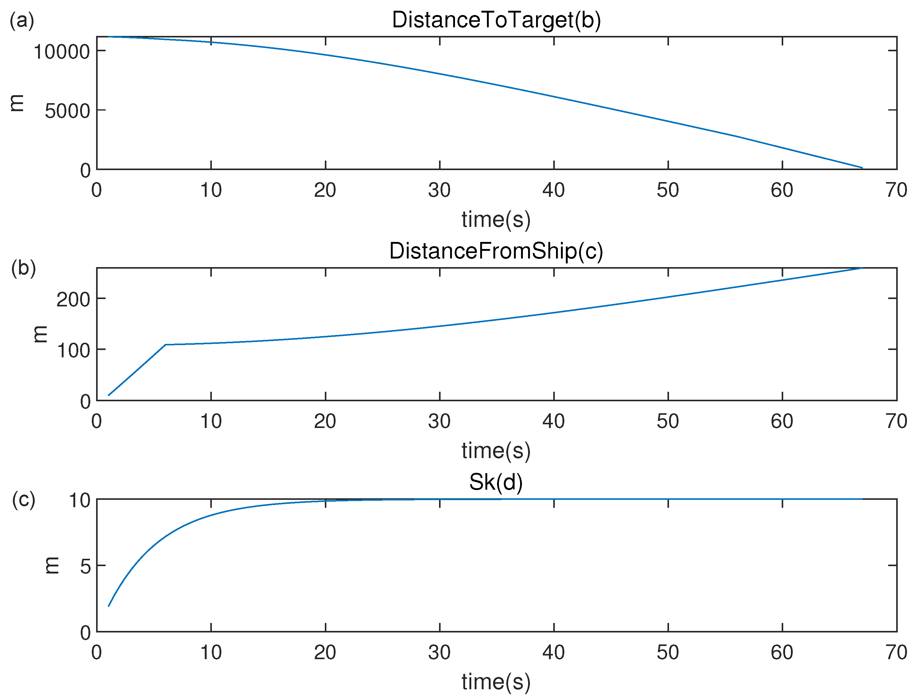
Figure 7a plots the distance between the virtual agent and the target as time elapses. The relative distance keeps decreasing as time elapses. Figure 7b depicts the distance between the virtual agent and the ship as time elapses. You can see that the virtual agent stays close to the safety distance $\beta$ while protecting the ship. Figure 7c depicts the side length as time elapses. As time elapses, the side length increases to $\Delta$.

6.3.1. The Effect of Changing System PARAMETERS (Number of Drones and Noise Strength)

We discuss the effect of the number of drones. We also present the effect of noise on the control performance. Let $N_s$ denote the standard deviation of measurement noise. In Equation (12), the measurement noise ${\mathbf{v}}_k$ is generated with ${\mathbf{v}}_k\sim \mathcal{N}(\mathbf{0},{\mathbf{R}}_k)$, where ${\mathbf{R}}_k$ is the diagonal matrix such that every diagonal element is $N_s^2$. This implies that the standard deviation of measurement noise is $N_s$ in meters.

Table 1. MC simulation results. The effect of changing system parameters, G and $N_s$.

G	${\mathit{N}}_{\mathit{s}}$	cR	eD	sT
3	1	100	95	57
1	1	100	108	57
3	10	100	94	57
1	10	60	105	57

summarizes the MC simulation results representing the effect of system parameters. We apply three metrics ($captureRate\left(cR\right)$, $endDist\left(eD\right)$, and $simTime\left(sT\right)$) to analyze the proposed controls. As the number of drones increases, $captureRate$ increases in general. This is due to the fact that as we deploy more drones, the area covered by the drones increases. Furthermore, as the measurement noise $N_s$ increases to 10 meters, the $captureRate$ decreases. Note that an MC simulation ends when the distance between a drone and the target is less than $\Delta =10$ m.

6.3.2. Comparison with Other State-of-the-Art Guidance Laws (Scenario 1)

To the best of our knowledge, this article is novel in developing a ship defense approach using clustered multiple drones. For comparison, we consider the case where only one drone is used, and the virtual agent applies the 3D PNG law in Section 6.2 to capture the target. We also consider the case where only one drone is used, and the drone applies the 3D Motion Camouflage Guidance (MCG) law in [18] to chase the target. We further consider the case where only one drone is used, and the drone applies the 3D Command to Line-Of-Sight (CLOS) guidance law in [53].

Table 2. Comparison with other state-of-the-art controls (Scenario 1).

Control	${\mathit{N}}_{\mathit{s}}$	cR	eD	sT
$PR{O}_3$	1	100	95	57
$PR{O}_1$	1	100	108	57
$PNG$	1	0	280	57
$MCG$	1	0	280	57
$CLOS$	1	20	276	56

shows the MC simulation comparison results of Scenario 1. We run $mC$ MC simulations per each control law. Let $PR{O}_q$ indicate the proposed guidance law using $G=q$ in Equation (4). Note that only one drone is used in $PR{O}_1$. Moreover, nine drones are used in $PR{O}_3$.

In Table 2, $MCG$ presents the case where the 3D MCG law is used. $PNG$ presents the case where the 3D PNG law is used. $CLOS$ presents the case where the 3D CLOS law is used. See that the proposed control outperforms all other state-of-the-art controls.

Note that Equation (31) can be satisfied even when $v_{max}<v_k^t$. This implies that even slow drones can capture a fast target when the drones stay close to the ship while staying in the lineState at all times. However, other state-of-the-art guidance laws ($MCG$, $PNG$, and $CLOS$) make a drone continue to chase the target. This maneuver makes the drone move away from the ship, which is not desirable for capturing a fast target using a slow interceptor.

Other state-of-the-art guidance laws ($MCG$, $PNG$, and $CLOS$) make a single drone chase the target. In our paper, we let multiple drones form a planar grid formation, which can be considered a “net” structure to capture the incoming target. The target may perform elusive maneuvers, and there may be measurement noise in measuring the target position. By maximizing the grid formation size, the capture rate is 100, even when there exists error in the prediction of the target’s position. Since the target is guided to hit its goal (ship), the drones can effectively block the target using this grid formation.

6.4. Scenario 2

We introduce Scenario 2 in Figure 8. The distinctions of Figure 8 from Figure 4 are as follows. As the relative distance between the target and the ship is less than 3000 m, the target moves towards the ship directly while increasing its speed to 240 m/s.

Figure 8 depicts the result of one MC simulation. We set $G=5$ in Equation (4), i.e., we use $G^2=25$ drones in total. The position of every drone at every 3 s is depicted as circles with distinct colors. A red asterisk depicts the position of the virtual agent at every 3 s. Figure 8 shows the case where the target is captured by a drone.

Figure 9 is the enlarged figure of Figure 8. The position of every drone at every 3 s is depicted as circles with distinct colors. See that the grid formation is generated to protect the ship from the incoming target.

Considering the scenario in Figure 9, Figure 10 removes the plots for the target’s positions in order to see the drones’ maneuvers clearly. The position of every drone at every 3 s is depicted as circles with distinct colors. A red asterisk depicts the position of the virtual agent at every 3 s. The position of the ship at every 3 s is indicated by red diamonds. A black asterisk presents the target’s position when the target is hit by a drone.

Figure 11a depicts the distance between the virtual agent and the target as time elapses. See that the relative distance continuously decreases over time. Figure 11b depicts the distance between the virtual agent and the ship as time elapses. See that the virtual agent stays close to the safety distance $\beta$ while protecting the ship. Figure 11c depicts the side length as time elapses. As time elapses, the side length increases to $\Delta$.

Comparison with Other State-of-the-Art Guidance Laws (Scenario 2)

Table 3. Comparison with other state-of-the-art controls (Scenario 2).

Control	${\mathit{N}}_{\mathit{s}}$	cR	eD	sT
$PR{O}_5$	10	100	247	67
$PR{O}_1$	10	95	260	67
$PNG$	10	0	339	68
$MCG$	10	0	339	68
$CLOS$	10	0	339	68

shows the MC comparison results of Scenario 2. In this table, $N_s$ denotes the measurement noise. We run $mC$ MC simulations per each control law.

In Table 3, $PR{O}_q$ indicates the proposed guidance law using $G=q$ in (4). Note that only one drone is used in $PR{O}_1$. Moreover, 25 drones are used in $PR{O}_5$.

Table 3 shows that the proposed control outperforms all other controls. $MCG$, $PNG$, and $CLOS$ make a drone keep chasing the target. This maneuver makes the drone move away from the ship, which is not desirable for capturing a fast target using a slow interceptor.

Other state-of-the-art guidance laws ($MCG$, $PNG$, and $CLOS$) make a single drone chase the target. Our strategy is to let multiple drones form a planar grid formation, which can be considered as a “net” for capturing the incoming target. By maximizing the grid formation size, the captureRate is 100 even when there exists error in the prediction of the target’s position.

7. Conclusions

This article introduces a multi-agent guidance law so that a formation of drones protects the ship from an incoming high-speed target. The drones generate a planar grid formation, whose center is guided to remain on the line connecting the target and the ship. Moreover, the planar formation is generated to be perpendicular to the line segment connecting the target and the formation center. Since a target heads towards its goal at least in the terminal phase, maintaining a position on this line segment is effective in protecting the ship.

We enable slow drones to capture a fast target by letting the drones stay close to the ship while staying in the lineState at all times. This blocking strategy is desirable considering the energy consumption of the interceptor since an interceptor does not have to move far from the ship.

We control the drone formation based on the prediction of the target’s position after one sample-index in the future. Since we use a grid formation of drones, we can increase the capture rate even when the target prediction is erroneous.

As far as we know, this article is novel in developing a ship defense approach using multiple clustered drones. In addition, our paper is novel in addressing the 3D formation control that can handle uncertainty in the target prediction. The effectiveness of our multi-agent guidance law is shown by comparing it with other state-of-the-art guidance laws under MATLAB simulations. We verify that the proposed multi-drone guidance scheme increases the capture probability significantly compared to the case where a single interceptor is used. In the future, we will do experiments to verify our multi-agent guidance law using real drones.

In practice, the presence of wind can affect and modify a drone’s path. Many papers handled how to control a drone under the effect of wind [54,55,56,57,58]. The authors of [54] improved the accelerated A-star algorithm with a converted wind vector, and [55] addressed the problem of a drone’s path planning operating in complex four-dimensional (time and spatially varying) wind-fields. Additionally, refs. [56,57,58] handled adaptive path planning in windy conditions. The authors of [58] added a wind model to the existing path planning algorithm and combined it with a drone’s control systems. In the future, we will combine the proposed guidance scheme with a wind model so that multiple drones can safely maneuver in time-varying wind-fields.

Note that the proposed guidance scheme can be applied to protect an entity other than a ship, as long as the goal of the target is known a priori. For instance, the proposed multi-agent guidance law can be generalized to protect any vehicles, such as tanks or ground stations.

References

- Kim, J.; Gadsden, S.A.; Wilkerson, S.A. A Comprehensive Survey of Control Strategies for Autonomous Quadrotors. Can. J. Electr. Comput. Eng. 2020, 43, 3–16. [Google Scholar] [CrossRef]
- Santana, L.V.; Brandao, A.S.; Sarcinelli-Filho, M. Outdoor waypoint navigation with the AR. Drone quadrotor. In Proceedings of the 2015 International Conference on Unmanned Aircraft Systems (ICUAS), Denver, CO, USA, 9–12 June 2015; pp. 303–311. [Google Scholar]
- Mellinger, D.; Michael, N.; Kumar, V. Trajectory generation and control for precise aggressive maneuvers with quadrotors. Int. J. Robot. Res. 2012, 31, 664–674. [Google Scholar] [CrossRef]
- Bar-Shalom, Y.; Fortmann, T.E. Tracking and Data Association; Academic Press: Orlando, FL, USA, 1988. [Google Scholar]
- Minaeian, S.; Liu, J.; Son, Y. Vision-Based Target Detection and Localization via a Team of Cooperative UAV and UGVs. IEEE Trans. Syst. Man Cybern. Syst. 2016, 46, 1005–1016. [Google Scholar] [CrossRef]
- Svec, P.; Thakur, A.; Raboin, E.; Shah, B.C.; Gupta, S.K. Target following with motion prediction for unmanned surface vehicle operating in cluttered environments. Auton. Robot. 2014, 36, 383–405. [Google Scholar] [CrossRef]
- Kim, J.; Kim, S.; Choo, Y. Stealth Path Planning for a High Speed Torpedo-Shaped Autonomous Underwater Vehicle to Approach a Target Ship. Cyber Phys. Syst. 2018, 4, 1–16. [Google Scholar] [CrossRef]
- Kim, J. Target Following and Close Monitoring Using an Unmanned Surface Vehicle. IEEE Trans. Syst. Man, Cybern. Syst. 2018, 50, 4233–4242. [Google Scholar] [CrossRef]
- Xu, Y.; Basset, G. Sequential virtual motion camouflage method for nonlinear constrained optimal trajectory control. Automatica 2012, 48, 1273–1285. [Google Scholar] [CrossRef]
- Srinivasan, M.V.; Davey, M. Strategies for Active Camouflage of Motion. Proc. R. Soc. B Biol. Sci. 1995, 259, 19–25. [Google Scholar]
- Mizutani, A.; Chahl, J.; Srinivasan, M. Insect behaviour: Motion camouflage in dragonflies. Nature 2003, 423, 604. [Google Scholar] [CrossRef]
- Rano, I. Direct collocation for two dimensional motion camouflage with non-holonomic, velocity and acceleration constraints. In Proceedings of the 2013 IEEE International Conference on Robotics and Biomimetics (ROBIO), Shenzhen, China, 13–14 December 2013; pp. 109–114. [Google Scholar] [CrossRef]
- Justh, E.; Krishnaprasad, P. Steering laws for motion camouflage. Proc. R. Soc. A 2006, 462, 3629–3643. [Google Scholar] [CrossRef] [Green Version]
- Ghose, K.; Horiuchi, T.K.; Krishnaparasad, P.S.; Moss, C.F. Ecolocating bats use a nearly time-optimal strategy to intercept prey. PLoS Biol. 2006, 4, 865–873. [Google Scholar] [CrossRef] [PubMed] [Green Version]
- Anderson, A.J.; McOwan, P.W. Model of a predatory stealth behaviour camouflaging motion. Proc. R. Soc. B 2003, 270, 489–495. [Google Scholar] [CrossRef] [PubMed] [Green Version]
- Kim, J. Controllers to Chase a High-Speed Evader Using a Pursuer with Variable Speed. Appl. Sci. 2018, 8, 1976. [Google Scholar] [CrossRef] [Green Version]
- Galloway, K.S.; Justh, E.W.; Krishnaprasad, P.S. Motion camouflage in a stochastic setting. In Proceedings of the IEEE International Conference on Decision and Control (CDC), New Orleans, LA, USA, 12–14 December 2007; pp. 1652–1659. [Google Scholar]
- Reddy, P.V.; Justh, E.W.; Krishnaprasad, P.S. Motion camouflage in three dimensions. In Proceedings of theDecision and Control, San Diego, CA, USA, 13–15 December 2006; IEEE: Piscataway, NJ, USA, 2006; pp. 3327–3332. [Google Scholar]
- Halder, U.; Dey, B. Biomimetic Algorithms for Coordinated Motion: Theory and Implementation. In Proceedings of the International Conference on Robotics and Automation (ICRA), Seattle, DC, USA, 26–30 May 2015; IEEE: Piscataway, NJ, USA, 2015; pp. 5426–5432. [Google Scholar]
- Oh, J.; Ha, I. Capturability of the 3-dimensional pure PNG law. IEEE Trans. Aerosp. Electron. Syst. 1999, 35, 491–503. [Google Scholar]
- Song, S.; Ha, I. A lyapunov-like approach to performance analysis of 3-dimensional pure PNG laws. IEEE Trans. Aerosp. Electron. Syst. 1994, 30, 238–248. [Google Scholar] [CrossRef]
- Liu, D.; Lee, M.C.; Pun, C.M.; Liu, H. Analysis of Wireless Localization in Non-Line-of-Sight Conditions. IEEE Trans. Veh. Technol. 2013, 62, 1484–1492. [Google Scholar] [CrossRef]
- Prasanna, H.M.; Ghose, D. Retro-Proportional-Navigation: A new guidance law for interception of high-speed targets. J. Guid. Control Dyn. 2012, 35, 377–386. [Google Scholar] [CrossRef]
- Mischiati, M.; Krishnaprasad, P.S. Mutual motion camouflage in 3D. In Proceedings of the 18th IFAC World Congress, Milan, Italy, 28 August–2 September 2011; pp. 4483–4488. [Google Scholar]
- Alonso-Mora, J.; Montijano, E.; N?geli, T.; Hilliges, O.; Schwager, M.; Rus, D. Distributed multi-robot formation control in dynamic environments. Auton. Robot. 2019, 43, 1079–1100. [Google Scholar] [CrossRef] [Green Version]
- Ji, M.; Muhammad, A.; Egerstedt, M. Leader-based multi-agent coordination: Controllability and optimal control. In Proceedings of the American Control Conference, Minneapolis, MN, USA, 14–16 June 2006; pp. 1358–1363. [Google Scholar]
- Kim, J. Cooperative Exploration and Networking While Preserving Collision Avoidance. IEEE Trans. Cybern. 2017, 47, 4038–4048. [Google Scholar] [CrossRef]
- Kim, J. Capturing intruders based on Voronoi diagrams assisted by information networks. Int. J. Adv. Robot. Syst. 2017, 14, 1729881416682693. [Google Scholar] [CrossRef]
- Kim, J. Cooperative Exploration and Protection of a Workspace Assisted by Information Networks. Ann. Math. Artif. Intell. 2014, 70, 203–220. [Google Scholar] [CrossRef]
- Parker, L.E.; Kannan, B.; Fu, X.; Tang, Y. Heterogeneous mobile sensor net deployment using robot herding and line-of-sight formations. In Proceedings of the Intelligent Robots and Systems, Las Vegas, NV, USA, 27 October–1 November 2003; Volume 3, pp. 2488–2493. [Google Scholar]
- Mirzaei, F.M.; Mourikis, A.I.; Roumeliotis, S.I. On the Performance of Multi-robot Target Tracking. In Proceedings of the 2007 IEEE International Conference on Robotics and Automation, Roma, Italy, 10–14 April 2007; pp. 3482–3489. [Google Scholar] [CrossRef]
- Hausman, K.; Muller, J.; Hariharan, A.; Ayanian, N.; Sukhatme, G.S. Cooperative multi-robot control for target tracking with onboard sensing. Int. J. Robot. Res. 2015, 34, 1660–1677. [Google Scholar] [CrossRef]
- Fonod, R.; Shima, T. Wingman-based Estimation and Guidance for a Sensorless PN-Guided Pursuer. IEEE Trans. Aerosp. Electron. Syst. 2019, 56, 1754–1766. [Google Scholar] [CrossRef] [Green Version]
- Fonod, R.; Shima, T. Blinding Guidance Against Missiles Sharing Bearings-Only Measurements. IEEE Trans. Aerosp. Electron. Syst. 2018, 54, 205–216. [Google Scholar] [CrossRef]
- Jeon, I.; Lee, J.; Tahk, M. Homing guidance law for cooperative attack of multiple missiles. J. Guid. Control Dyn. 2010, 33, 275–280. [Google Scholar] [CrossRef]
- Zhang, T.; Yang, J. Guidance law of multiple missiles for cooperative simultaneous attack against maneuvering target. In Proceedings of the 2018 37th Chinese Control Conference (CCC), Wuhan, China, 25–27 July 2018; pp. 4536–4541. [Google Scholar] [CrossRef]
- Lee, C.H.; Tsourdos, A. Cooperative Control for Multiple Interceptors to Maximize Collateral Damage. IFAC-PapersOnLine 2018, 51, 56–61. [Google Scholar] [CrossRef]
- Wang, L.; Liu, K.; Yao, Y.; He, F. A Design Approach for Simultaneous Cooperative Interception Based on Area Coverage Optimization. Drones 2022, 6, 156. [Google Scholar] [CrossRef]
- Fossen, T.I. Guidance and Control of OCEAN Vehicles; John Wiley and Sons: Hoboken, NJ, USA, 1994. [Google Scholar]
- Garcia de Marina, H.; Cao, M.; Jayawardhana, B. Controlling Rigid Formations of Mobile Agents Under Inconsistent Measurements. IEEE Trans. Robot. 2015, 31, 31–39. [Google Scholar] [CrossRef] [Green Version]
- Krick, L.; Broucke, M.E.; Francis, B.A. Stabilization of infinitesimally rigid formations of multi-robot networks. In Proceedings of the 2008 47th IEEE Conference on Decision and Control, Cancun, Mexico, 9–11 December 2008; pp. 477–482. [Google Scholar]
- Paley, D.A.; Zhang, F.; Leonard, N.E. Cooperative Control for Ocean Sampling: The Glider Coordinated Control System. IEEE Trans. Control Syst. Technol. 2008, 16, 735–744. [Google Scholar] [CrossRef]
- Ji, M.; Egerstedt, M. Distributed Coordination Control of Multiagent Systems While Preserving Connectedness. IEEE Trans. Robot. 2007, 23, 693–703. [Google Scholar] [CrossRef]
- Kim, J. Constructing 3D Underwater Sensor Networks without Sensing Holes Utilizing Heterogeneous Underwater Robots. Appl. Sci. 2021, 11, 4293. [Google Scholar] [CrossRef]
- Kim, J.; Kim, S. Motion control of multiple autonomous ships to approach a target without being detected. Int. J. Adv. Robot. Syst. 2018, 15, 1729881418763184. [Google Scholar] [CrossRef]
- Luo, S.; Kim, J.; Parasuraman, R.; Bae, J.H.; Matson, E.T.; Min, B.C. Multi-robot rendezvous based on bearing-aided hierarchical tracking of network topology. Ad Hoc Netw. 2019, 86, 131–143. [Google Scholar] [CrossRef]
- Ristic, B.; Arulampalam, S.; Gordon, N. Beyond the Kalman Filter: Particle Filters for Tracking Applications; Artech House Radar Library: Boston, MA, USA, 2004. [Google Scholar]
- MacAlpine, P.; Price, E.; Stone, P. SCRAM: Scalable Collision-avoiding Role Assignment with Minimal-Makespan for Formational Positioning. In Proceedings of the AAAI Conference on Artificial Intelligence, Austin, TX, USA, 25–30 January 2015; Volume 29. [Google Scholar]
- Chakravarthy, A.; Ghose, D. Obstacle avoidance in a dynamic environment: A collision cone approach. IEEE Trans. Syst. Man Cybern. 1998, 28, 562–574. [Google Scholar] [CrossRef] [Green Version]
- Svec, P.; Shah, B.C.; Bertaska, I.R.; Alvarez, J.; Sinisterra, A.J.; von Ellenrieder, K.; Dhanak, M.; Gupta, S.K. Dynamics-aware target following for an automomous surface vehicle pperating under Colregs in civilian traffic. In Proceedings of the IEEE/RSJ International Conference on Intelligent Robots and Systems (IROS), Tokyo, Japan, 3–7 November 2013; pp. 3871–3878. [Google Scholar]
- Chang, D.E.; Shadden, S.C.; Marsden, J.E.; Olfati-Saber, R. Collision Avoidance for Multiple Agent Systems. In Proceedings of the IEEE International Conference on Decision and Control, Maui, HI, USA, 9–12 December 2003; pp. 539–543. [Google Scholar]
- Lalish, E.; Morgansen, K. Distributed reactive collision avoidance. Auton. Robot 2012, 32, 207–226. [Google Scholar] [CrossRef]
- Zahra, B.F.T.; Shah, S.I.A. Integrated CLOS and PN Guidance for Increased Effectiveness of Surface to Air Missiles. INCAS Bull. 2017, 9, 141–156. [Google Scholar]
- Selecký, M.; Váňa, P.; Rollo, M.; Meiser, T. Wind Corrections in Flight Path Planning. Int. J. Adv. Robot. Syst. 2013, 10, 248. [Google Scholar] [CrossRef] [Green Version]
- Chakrabarty, A.; Langelaan, J. UAV flight path planning in time varying complex wind-fields. In Proceedings of the 2013 American Control Conference, Washington, DC, USA, 17–19 June 2013; pp. 2568–2574. [Google Scholar]
- Coombes, M.; Chen, W.H.; Liu, C. Boustrophedon coverage path planning for UAV aerial surveys in wind. In Proceedings of the 2017 International Conference on Unmanned Aircraft Systems (ICUAS), Miami, FL, USA, 13–16 June 2017; pp. 1563–1571. [Google Scholar]
- Coombes, M.; Fletcher, T.; Chen, W.H.; Liu, C. Optimal Polygon Decomposition for UAV Survey Coverage Path Planning in Wind. Sensors 2018, 18, 2132. [Google Scholar] [CrossRef] [Green Version]
- McGee, T.; Hedrick, J. Path planning and control for multiple point surveillance by an unmanned aircraft in wind. In Proceedings of the 2006 American Control Conference, Minneapolis, MN, USA, 14–16 June 2006; pp. 4261–4266. [Google Scholar]
Figure 1.
The case where the ship moves as the time index changes from k to . The ship positions are indicated by crosses. In this figure, , , and are depicted.
Figure 2.
Block diagram of the proposed multi-drone guidance law.
Figure 3.
The case where and meet at .
Figure 4.
The result of one MC simulation using the proposed multi-agent guidance law. The proposed multi-agent guidance law is applied to hit the target. The position of every drone at every 3 s is depicted as circles with distinct colors. A red asterisk depicts the position of the virtual agent at every 3 s. The target’s position at every 3 s is marked as blue circles. The position of the ship at every 3 s is indicated by red diamonds.
Figure 5.
The enlarged figure of Figure 4. The position of every drone at every 3 s is depicted as circles with distinct colors. The drones generate a grid formation for protection against the incoming target.
Figure 6.
Considering the scenario in Figure 5, we remove the plots for the target’s positions in order to see the drones’ maneuvers clearly. The position of every drone at every 3 s is depicted as circles with distinct colors. A red asterisk depicts the position of the virtual agent at every 3 s. The position of the ship at every 3 s is indicated by red diamonds. A black asterisk presents the target’s position when the target is hit by a drone.
Figure 7.
The result of one MC simulation using grid formation. The proposed guidance law is applied to hit the target. (a) depicts the distance between the virtual agent and the target as time elapses. The relative distance keeps decreasing as time elapses. (b) plots the distance between the virtual agent and the ship as time elapses. See that the virtual agent stays close to the safety distance while protecting the ship. (c) depicts the side length as time elapses.
Figure 8.
The result of one MC simulation using the proposed grid formation. The position of every drone at every 3 s is depicted as circles with distinct colors. A red asterisk depicts the position of the virtual agent at every 3 s.
Figure 9.
The enlarged figure of Figure 8. The position of every drone at every 3 s is depicted as circles with distinct colors. See that the grid formation is generated to protect the ship from the incoming target.
Figure 10.
Considering the scenario in Figure 9, we remove the plots for the target’s positions in order to see the drones’ maneuvers clearly. The position of every drone at every 3 s is depicted as circles with distinct colors. A red asterisk depicts the position of the virtual agent at every 3 s. The position of the ship at every 3 s is indicated by red diamonds. A black asterisk presents the target’s position when the target is hit by a drone.
Figure 11.
(a) depicts the distance between the virtual agent and the target as time elapses. See that the relative distance continuously decreases over time. (b) plots the distance between the virtual agent and the ship as time elapses. See that the virtual agent stays close to the safety distance while protecting the ship. (c) depicts the side length as time elapses.