
Modelling of Electric Bus Operation and Charging Process: Potential Contribution of Local Photovoltaic Production
 , ,
, ,  , and
, and
Abstract
:Featured Application
Abstract
1. Introduction
- A bus consumption model that considers the influence of the battery capacity on the bus gross weight and thus on the bus consumption;
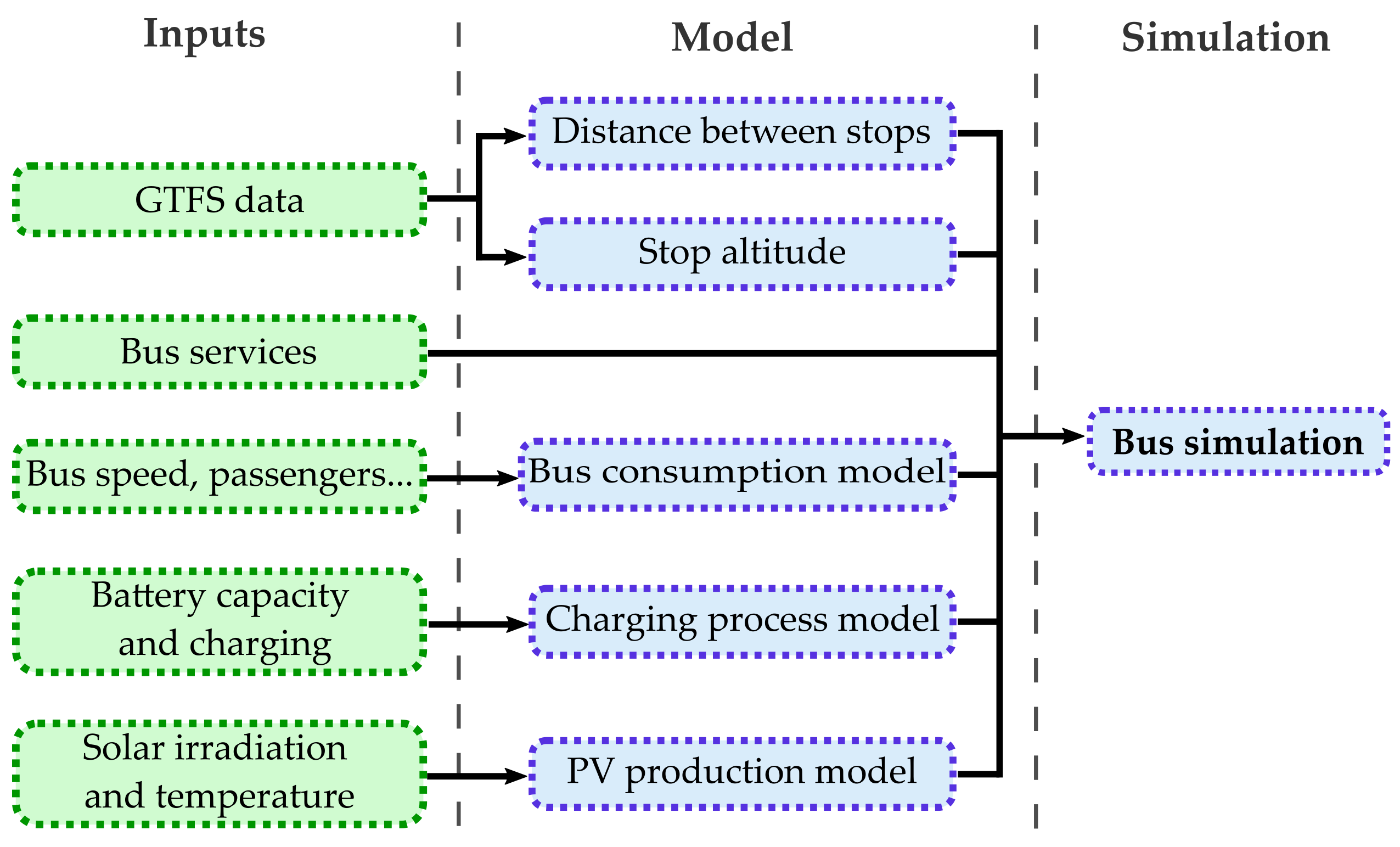
- Modelling of a bus network is presented based on General Transit Feed Specification (GTFS) data;
- A sequential simulation of the EB operation is performed in order to analyse the influence of the charging scenarios on the quality of transportation services (delay indicator);
- A comparison between bus energy demand and PV production in order to assess the potential of PV energy to reduce impacts of EB charging on the utility grid.
2. State of the Art of Scientific Literature
2.1. Research Positioning
2.2. Sizing of Charging Infrastructures
2.3. Photovoltaic Integration for Bus Charging
2.4. Discussion on the State of the Art
3. Modelling of the Bus Transportation Network
3.1. Definitions
3.2. Bus Consumption Modelling
3.2.1. Consumption Model
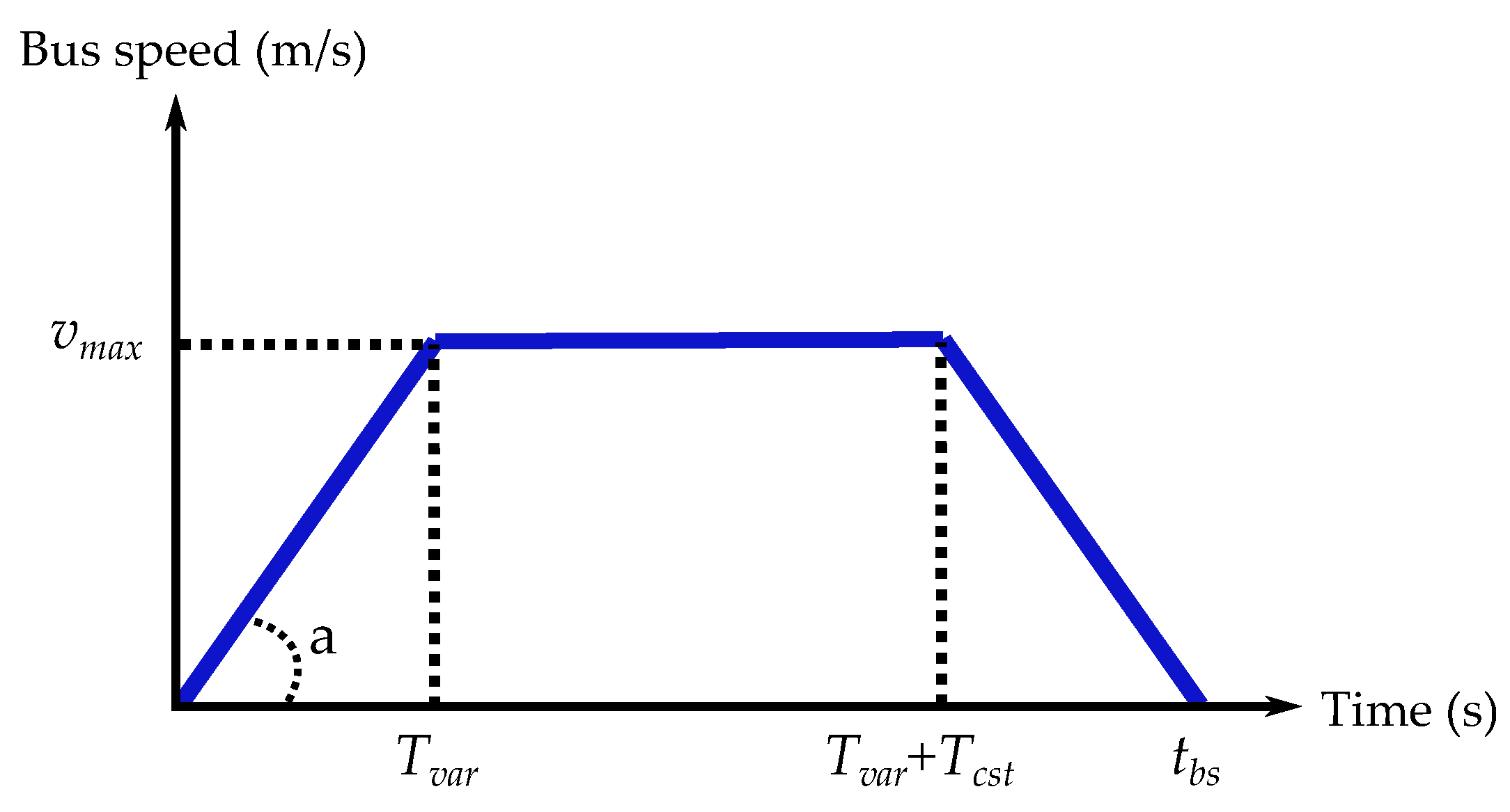
3.2.2. Speed Profile
3.3. Modelling of Charging Process
3.4. PV Production
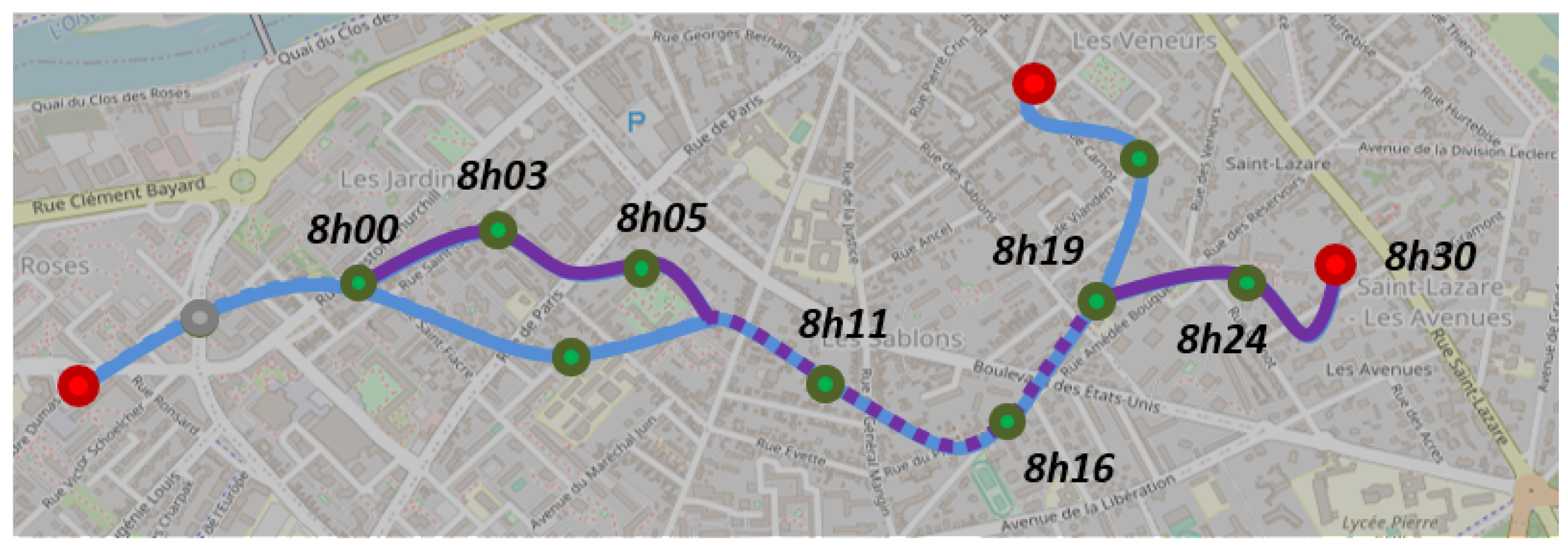
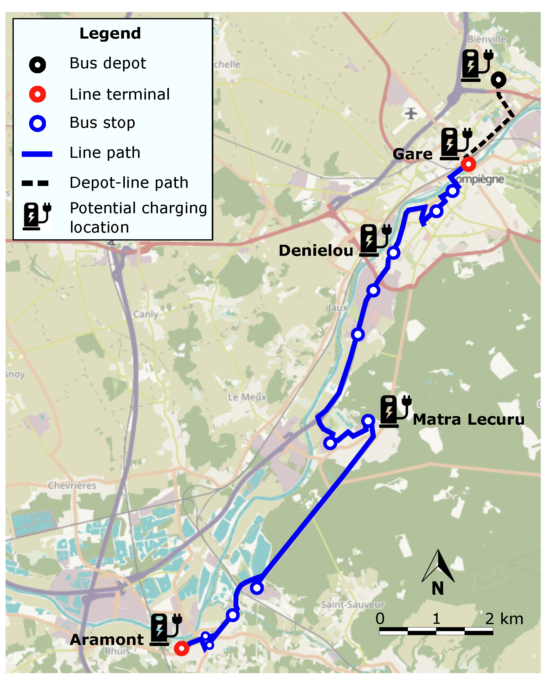
3.5. Bus Network Modelling
3.5.1. GTFS Data
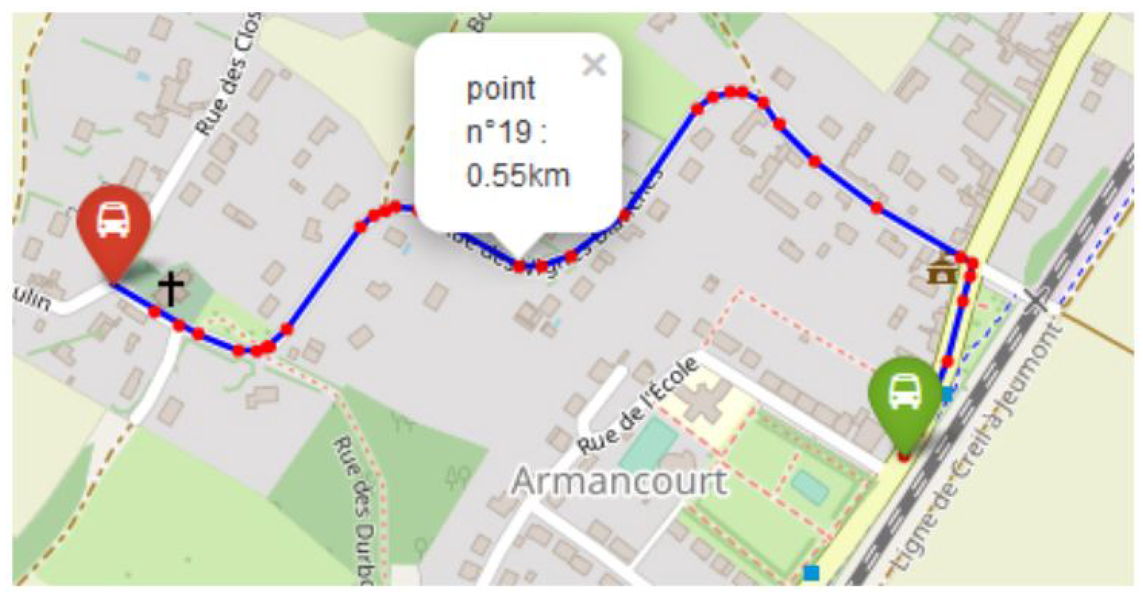
3.5.2. Post-Treatment of GTFS Data
3.6. Simulation of the Operation of Buses
4. Case Study
- Scenario 1: two chargers at the depot;
- Scenarios 2 and 2bis: two chargers at the depot and a charger at “Gare” and “Aramont” line terminals;
- Scenarios 3, 3bis, and 3ter: chargers at the terminals “Gare” and “Aramont”, and bus stops “Denielou” and “Matra Lecuru”.
5. Results
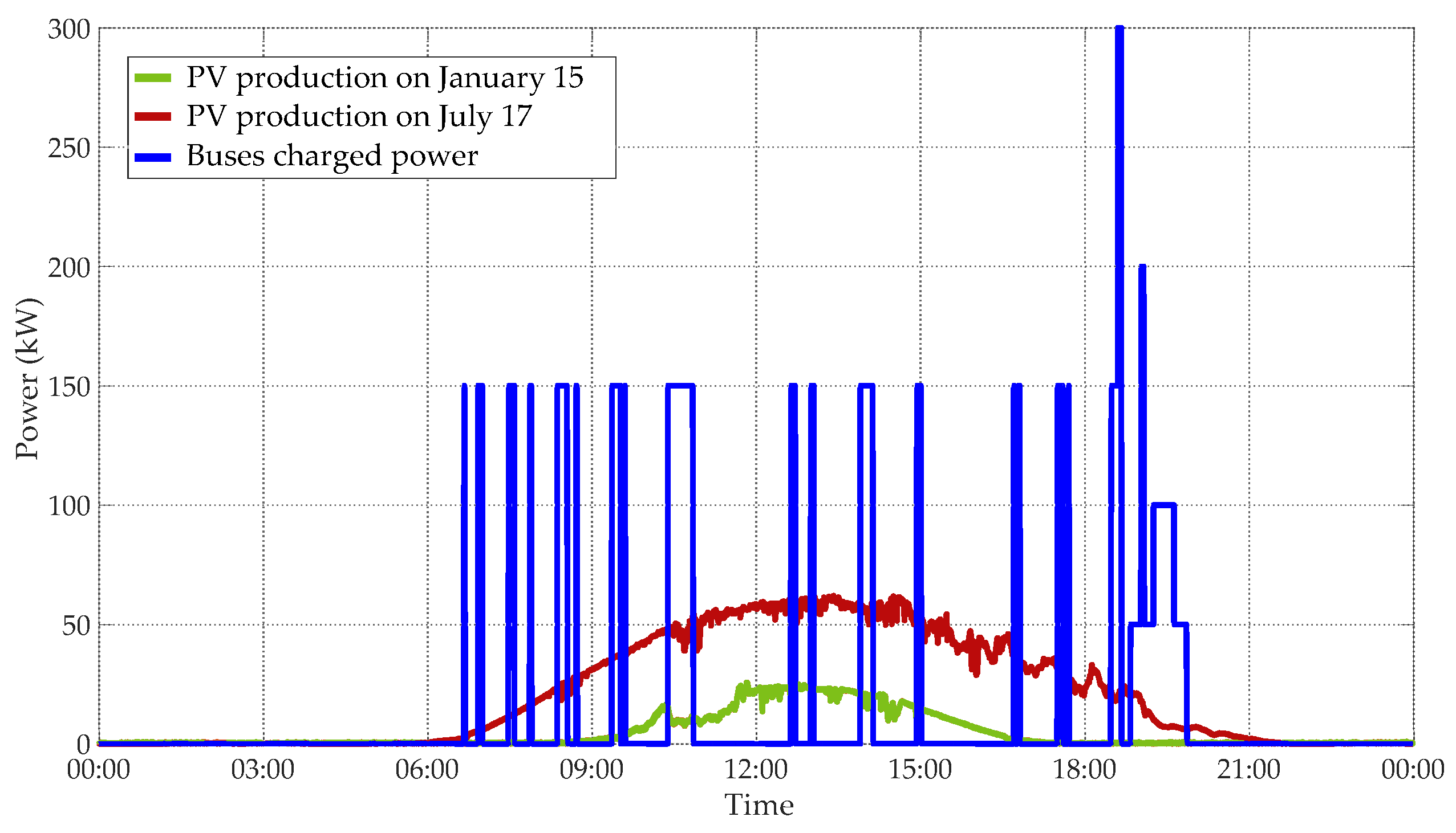
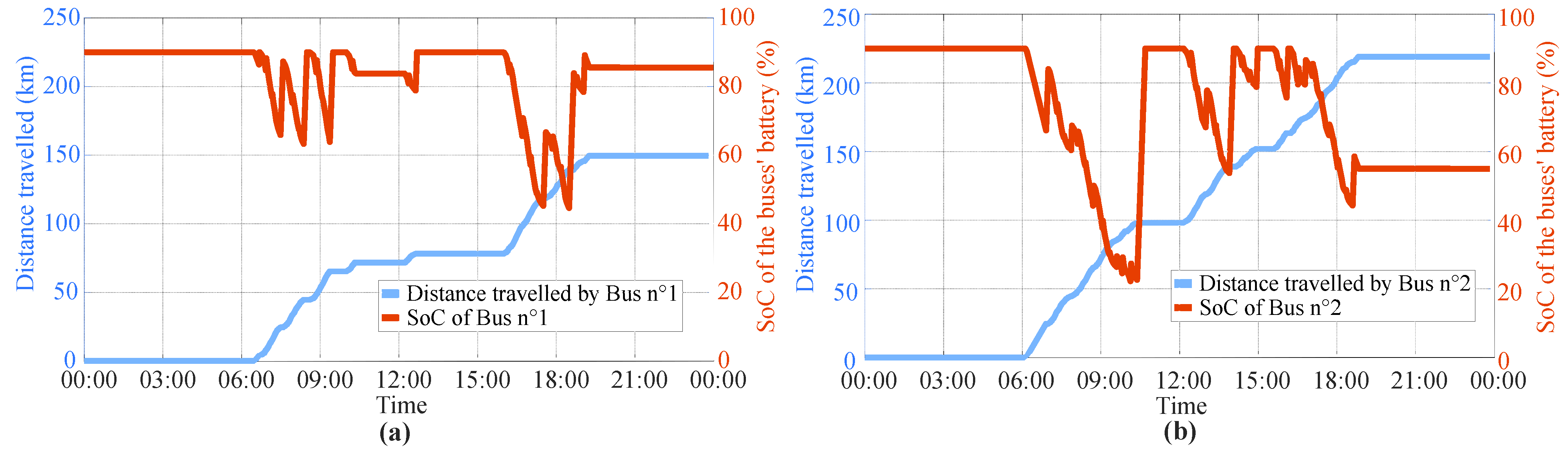
5.1. Scenario 1—Charge at the Bus Depot
5.2. Scenario 2—Charge at the Line Terminals
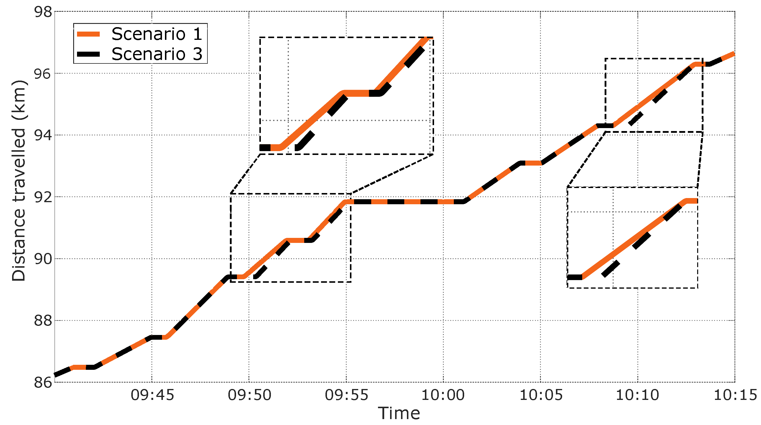
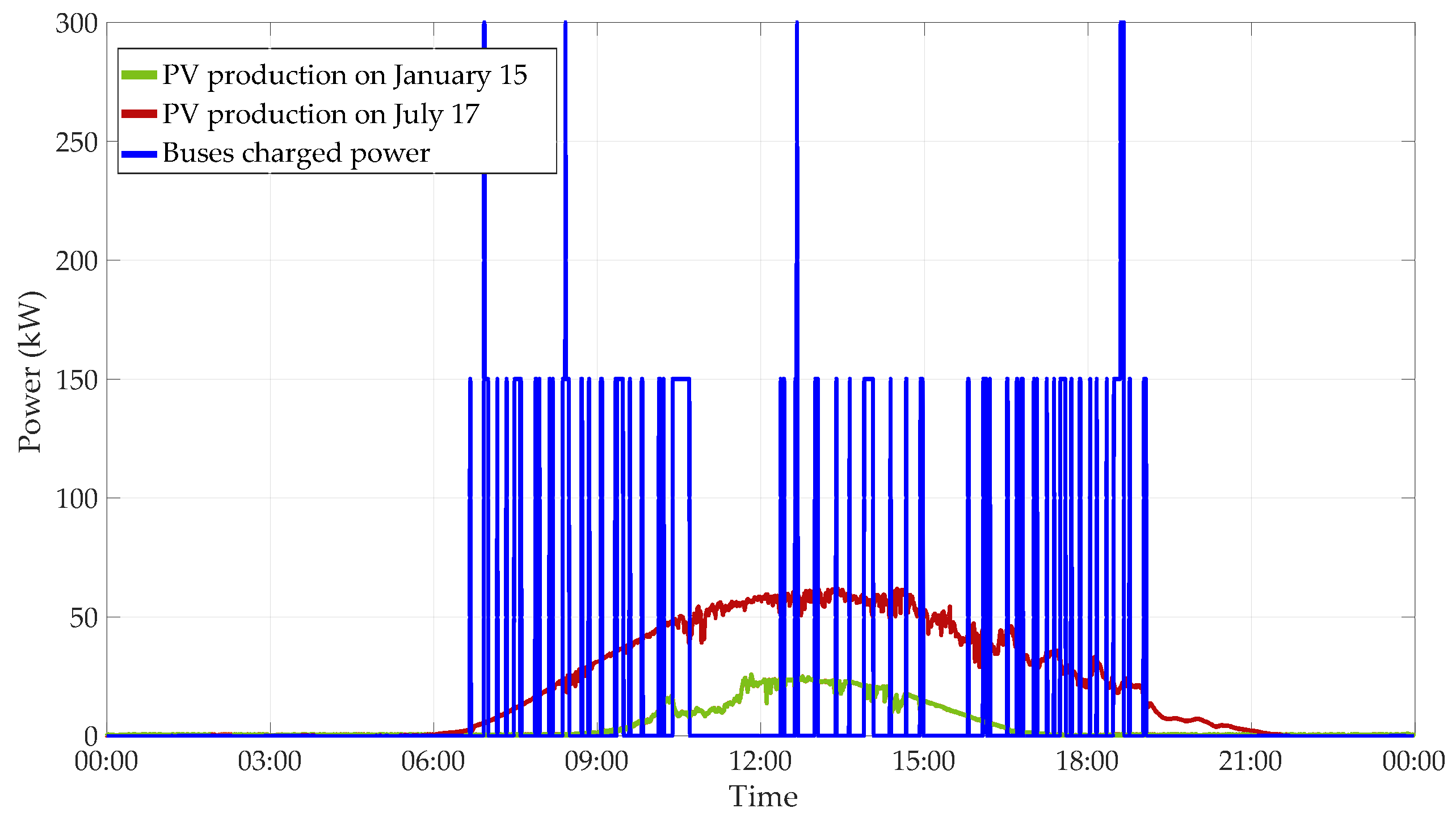
5.3. Scenario 3—Charge at Several Bus Stops
6. Discussion
7. Conclusions
Author Contributions
Funding
Institutional Review Board Statement
Informed Consent Statement
Data Availability Statement
Acknowledgments
Conflicts of Interest
References
- Avere-France. Guide Bus Électriques. Available online: https://www.avere-france.org/wp-content/uploads/site/documents/1632231132a3a1871eb36d22aa1acb6519aa46d6c7-GuidebuslectriquesAvere-Francevdef.pdf (accessed on 12 December 2022).
- UITP. ASSURED Clean Bus Report—An Overview of Clean Buses in Europe. Available online: https://cms.uitp.org/wp/wp-content/uploads/2022/04/ASSURED-Clean-Bus-Report-UITP-Final-v2.pdf (accessed on 12 December 2022).
- UITP. ZeEUS eBus Report #2—An Updated Overview of Electric Buses in Europe. Available online: https://zeeus.eu/uploads/publications/documents/zeeus-report2017-2018-final.pdf (accessed on 12 December 2022).
- Rodrigues, A.L.P.; Seixas, S.R.C. Battery-electric buses and their implementation barriers: Analysis and prospects for sustainability. Sustain. Energy Technol. Assess. 2022, 51, 101896. [Google Scholar] [CrossRef]
- Ji, J.; Bie, Y.; Zeng, Z.; Wang, L. Trip energy consumption estimation for electric buses. Commun. Transp. Res. 2022, 2, 100069. [Google Scholar] [CrossRef]
- He, Y.; Liu, Z.; Song, Z. Integrated charging infrastructure planning and charging scheduling for battery electric bus systems. Transp. Res. Part D Transp. Environ. 2022, 111, 103437. [Google Scholar] [CrossRef]
- TOSA. TOSA: Geneva’s Electrical Bus Innovation. Available online: https://www.intelligenttransport.com/transport-articles/71567/tosa-bus/ (accessed on 12 December 2022).
- Calstart. Zeroing in on ZEBs—2020 Edition. Available online: https://calstart.org/wp-content/uploads/2021/01/Zeroing_In_on_ZEBs_FINALREPORT_1262021.pdf (accessed on 12 December 2022).
- Perumal, S.S.G.; Lusby, R.M.; Larsen, J. Electric bus planning & scheduling: A review of related problems and methodologies. Eur. J. Oper. Res. 2022, 301, 395–413. [Google Scholar] [CrossRef]
- Manzolli, J.A.; Trovão, J.P.; Antunes, C.H. A review of electric bus vehicles research topics—Methods and trends. Renew. Sustain. Energy Rev. 2022, 159, 112211. [Google Scholar] [CrossRef]
- Boonraksa, T.; Boonraksa, P.; Marungsri, B. Optimal Capacitor Location and Sizing for Reducing the Power Loss on the Power Distribution Systems due to the Dynamic Load of the Electric Buses Charging System using the Artificial Bee Colony Algorithm. J. Electr. Eng. Technol. 2021, 16, 1821–1831. [Google Scholar] [CrossRef]
- Liu, K.; Gao, H.; Wang, Y.; Feng, T.; Li, C. Robust charging strategies for electric bus fleets under energy consumption uncertainty. Transp. Res. Part D Transp. Environ. 2022, 104, 103215. [Google Scholar] [CrossRef]
- Toniato, E.; Mehta, P.; Marinkovic, S.; Tiefenbeck, V. Peak load minimization of an e-bus depot: Impacts of user-set conditions in optimization algorithms. Energy Inform. 2021, 4, 23. [Google Scholar] [CrossRef]
- Gao, Z.; Lin, Z.; LaClair, T.J.; Liu, C.; Li, J.M.; Birky, A.K.; Ward, J. Battery capacity and recharging needs for electric buses in city transit service. Energy 2017, 122, 588–600. [Google Scholar] [CrossRef] [Green Version]
- Leone, C.; Sturaro, L.; Geroli, G.; Longo, M.; Yaici, W. Design and implementation of an electric skibus line in north Italy. Energies 2021, 14, 7925. [Google Scholar] [CrossRef]
- Hasan, M.M.; Avramis, N.; Ranta, M.; Saez-de Ibarra, A.; El Baghdadi, M.; Hegazy, O. Multi-Objective Energy Management and Charging Strategy for Electric Bus Fleets in Cities Using Various ECO Strategies. Sustainability 2021, 13, 7865. [Google Scholar] [CrossRef]
- Lotfi, M.; Pereira, P.; Paterakis, N.; Gabbar, H.; Catalao, J. Optimal Design of Electric Bus Transport Systems with Minimal Total Ownership Cost. IEEE Access 2020, 8, 119184–119199. [Google Scholar] [CrossRef]
- Kunith, A.; Mendelevitch, R.; Goehlich, D. Electrification of a city bus network—An optimization model for cost-effective placing of charging infrastructure and battery sizing of fast-charging electric bus systems. Int. J. Sustain. Transp. 2017, 11, 707–720. [Google Scholar] [CrossRef] [Green Version]
- Trocker, F.; Teichert, O.; Gallet, M.; Ongel, A.; Lienkamp, M. City-scale assessment of stationary energy storage supporting end-station fast charging for different bus-fleet electrification levels. J. Energy Storage 2020, 32, 101794. [Google Scholar] [CrossRef]
- Qin, N.; Gusrialdi, A.; Paul Brooker, R.; T-Raissi, A. Numerical analysis of electric bus fast charging strategies for demand charge reduction. Transp. Res. Part A Policy Pract. 2016, 94, 386–396. [Google Scholar] [CrossRef]
- Bie, Y.; Hao, M.; Guo, M. Optimal Electric Bus Scheduling Based on the Combination of All-Stop and Short-Turning Strategies. Sustainability 2021, 13, 1827. [Google Scholar] [CrossRef]
- Akaber, P.; Hughes, T.; Sobolev, S. MILP-based customer-oriented E-Fleet charging scheduling platform. IET Smart Grid 2021, 4, 215–223. [Google Scholar] [CrossRef]
- Lin, Y.; Zhang, K.; Shen, Z.J.M.; Ye, B.; Miao, L. Multistage large-scale charging station planning for electric buses considering transportation network and power grid. Transp. Res. Part C Emerg. Technol. 2019, 107, 423–443. [Google Scholar] [CrossRef]
- Tomizawa, Y.; Ihara, Y.; Kodama, Y.; Iino, Y.; Hayashi, Y.; Ikeda, O.; Yoshinaga, J. Multipurpose Charging Schedule Optimization Method for Electric Buses: Evaluation Using Real City Data. IEEE Access 2022, 10, 56067–56080. [Google Scholar] [CrossRef]
- Dalala, Z.; Al Banna, O.; Saadeh, O. The Feasibility and Environmental Impact of Sustainable Public Transportation: A PV Supplied Electric Bus Network. Appl. Sci. 2020, 10, 3987. [Google Scholar] [CrossRef]
- Arif, S.M.; Lie, T.T.; Seet, B.C.; Ahsan, S.M.; Khan, H.A. Plug-In Electric Bus Depot Charging with PV and ESS and Their Impact on LV Feeder. Energies 2020, 13, 2139. [Google Scholar] [CrossRef]
- Rafique, S.; Nizami, M.S.H.; Irshad, U.B.; Hossain, M.J.; Mukhopadhyay, S.C. A two-stage multi-objective stochastic optimization strategy to minimize cost for electric bus depot operators. J. Clean. Prod. 2022, 332, 129856. [Google Scholar] [CrossRef]
- Zhuang, P.; Liang, H. Stochastic Energy Management of Electric Bus Charging Stations with Renewable Energy Integration and B2G Capabilities. IEEE Trans. Sustain. Energy 2021, 12, 1206–1216. [Google Scholar] [CrossRef]
- Szcześniak, J.; Massier, T.; Gallet, M.; Sharma, A. Optimal Electric Bus Charging Scheduling for Local Balancing of Fluctuations in PV Generation. In Proceedings of the 2019 IEEE Innovative Smart Grid Technologies—Asia (ISGT Asia), Chengdu, China, 21–24 May 2019; pp. 2799–2804. [Google Scholar] [CrossRef]
- Santos, T.; Lobato, K.; Rocha, J.; Tenedório, J.A. Modeling Photovoltaic Potential for Bus Shelters on a City-Scale: A Case Study in Lisbon. Appl. Sci. 2020, 10, 4801. [Google Scholar] [CrossRef]
- Islam, S.M.M.; Salema, A.A.; Lim, J.M.Y. Design and sizing of solar PV plant for an electric bus depot in Malaysia. E3S Web Conf. 2020, 160, 02003. [Google Scholar] [CrossRef]
- Ren, H.; Ma, Z.; Ming Lun Fong, A.; Sun, Y. Optimal deployment of distributed rooftop photovoltaic systems and batteries for achieving net-zero energy of electric bus transportation in high-density cities. Appl. Energy 2022, 319, 119274. [Google Scholar] [CrossRef]
- Ren, H.; Ma, Z.; Fai Norman Tse, C.; Sun, Y. Optimal control of solar-powered electric bus networks with improved renewable energy on-site consumption and reduced grid dependence. Appl. Energy 2022, 323, 119643. [Google Scholar] [CrossRef]
- Agglomération de la Région de Compiègne. Fiche Horaire Ligne ARC Express—MAJ November 2021. Available online: https://www.agglo-compiegne.fr/sites/default/files/2021-11/Fiche%20horaire%20ARCexpress%20%20MAJ%20nov%202021.pdf (accessed on 12 December 2022).
- Hjelkrem, O.A.; Lervåg, K.Y.; Babri, S.; Lu, C.; Södersten, C.J. A battery electric bus energy consumption model for strategic purposes: Validation of a proposed model structure with data from bus fleets in China and Norway. Transp. Res. Part D Transp. Environ. 2021, 94, 102804. [Google Scholar] [CrossRef]
- Li, X.; Wang, T.; Li, J.; Tian, Y.; Tian, J. Energy Consumption Estimation for Electric Buses Based on a Physical and Data-Driven Fusion Model. Energies 2022, 15, 4160. [Google Scholar] [CrossRef]
- Ma, X.; Miao, R.; Wu, X.; Liu, X. Examining influential factors on the energy consumption of electric and diesel buses: A data-driven analysis of large-scale public transit network in Beijing. Energy 2021, 216, 119196. [Google Scholar] [CrossRef]
- El-Taweel, N.A.; Zidan, A.; Farag, H.E.Z. Novel Electric Bus Energy Consumption Model Based on Probabilistic Synthetic Speed Profile Integrated with HVAC. IEEE Trans. Intell. Transp. Syst. 2021, 22, 1517–1531. [Google Scholar] [CrossRef]
- Abdelaty, H.; Mohamed, M. A framework for BEB energy prediction using low-resolution open-source data-driven model. Transp. Res. Part D Transp. Environ. 2022, 103, 103170. [Google Scholar] [CrossRef]
- Asamer, J.; Graser, A.; Heilmann, B.; Ruthmair, M. Sensitivity analysis for energy demand estimation of electric vehicles. Transp. Res. Part D Transp. Environ. 2016, 46, 182–199. [Google Scholar] [CrossRef]
- Jefferies, D.; Göhlich, D. A Comprehensive TCO Evaluation Method for Electric Bus Systems Based on Discrete-Event Simulation Including Bus Scheduling and Charging Infrastructure Optimisation. World Electr. Veh. J. 2020, 11, 56. [Google Scholar] [CrossRef]
- Göhlich, D.; Fay, T.A.; Jefferies, D.; Lauth, E.; Kunith, A.; Zhang, X. Design of urban electric bus systems. Des. Sci. 2018, 4, e15. [Google Scholar] [CrossRef] [Green Version]
- Lajunen, A.; Lipman, T. Lifecycle cost assessment and carbon dioxide emissions of diesel, natural gas, hybrid electric, fuel cell hybrid and electric transit buses. Energy 2016, 106, 329–342. [Google Scholar] [CrossRef]
- Cigarini, F.; Fay, T.A.; Artemenko, N.; Göhlich, D. Modeling and experimental investigation of thermal comfort and energy consumption in a battery electric bus. World Electr. Veh. J. 2021, 12, 7. [Google Scholar] [CrossRef]
- Vepsäläinen, J.; Kivekäs, K.; Otto, K.; Lajunen, A.; Tammi, K. Development and validation of energy demand uncertainty model for electric city buses. Transp. Res. Part D Transp. Environ. 2018, 63, 347–361. [Google Scholar] [CrossRef]
- Kivekäs, K.; Lajunen, A.; Baldi, F.; Vepsäläinen, J.; Tammi, K. Reducing the Energy Consumption of Electric Buses with Design Choices and Predictive Driving. IEEE Trans. Veh. Technol. 2019, 68, 11409–11419. [Google Scholar] [CrossRef]
- Kessler, L.; Bogenberger, K. Dynamic traffic information for electric vehicles as a basis for energy-efficient routing. Transp. Res. Procedia 2019, 37, 457–464. [Google Scholar] [CrossRef]
- Gis, W.; Kruczyński, S.; Taubert, S.; Wierzejski, A. Studies of energy use by electric buses in SORT tests. Combust. Engines 2017, 170, 135–138. [Google Scholar] [CrossRef]
- Kammuang-lue, N.; Boonjun, J. Energy consumption of battery electric bus simulated from international driving cycles compared to real-world driving cycle in Chiang Mai. Energy Rep. 2021, 7, 344–349. [Google Scholar] [CrossRef]
- Algin, V.; Goman, A.; Skorokhodov, A. Main operational factors determining the energy consumption of the urban electric bus: Schematization and modelling. Top. Issues Mech. Eng. Collect. Sci. Pap. 2019, 8, 185–194. [Google Scholar] [CrossRef]
- Sechilariu, M.; Locment, F. Urban DC Microgrid: Intelligent Control and Power Flow Optimization; Elsevier Butterworth-Heinemann: Amsterdam, The Netherlands; Paris, France, 2016. [Google Scholar]
- Google Developers. Google Transit|Static Transit|GTFS Reference. Available online: https://developers.google.com/transit/gtfs/reference (accessed on 12 December 2022).
- OpenStreetMap. Available online: https://www.openstreetmap.org/ (accessed on 12 December 2022).
- Open-Elevation API. Available online: https://open-elevation.com/ (accessed on 12 December 2022).
- Czogalla, O.; Jumar, U. Design and control of electric bus vehicle model for estimation of energy consumption. IFAC PapersOnLine 2019, 52, 59–64. [Google Scholar] [CrossRef]
- Fiori, C.; Montanino, M.; Nielsen, S.; Seredynski, M.; Viti, F. Microscopic energy consumption modelling of electric buses: Model development, calibration, and validation. Transp. Res. Part D Transp. Environ. 2021, 98, 102978. [Google Scholar] [CrossRef]
- Agglomération de la Région de Compiègne. Plan des Lignes périurbaines de l’ARC. Available online: https://www.agglo-compiegne.fr/sites/default/files/2021-07/Depliant%20PLAN%20TIC%20MAJ%20JUILLET%202021%20periurbain.pdf (accessed on 12 December 2022).
- BYD Europe. BYD 12m eBus Europe. Available online: https://bydeurope.com/pdp-bus-model-12 (accessed on 12 December 2022).
- Electric Vehicle Charging Infrastructure. ABB Electric Bus Charging Station|Electric Truck Charging. Available online: https://new.abb.com/ev-charging/depot-connector-charging (accessed on 12 December 2022).
- Electric Vehicle Charging Infrastructure. ABB Pantograph Bus|Pantograph Up. Available online: https://new.abb.com/ev-charging/pantograph-up (accessed on 12 December 2022).


| Service n° | 1 | 2 | 1 | 2 | 1 | 2 | 2 | 2 | 1 | 2 | 1 |
|---|---|---|---|---|---|---|---|---|---|---|---|
| Trip n° | 1 | 2 | 3 | 4 | 5 | 6 | 7 | 8 | 9 | 10 | 11 |
| Bus stops | |||||||||||
| Gare | 06:42 | 07:54 | 08:36 | 09:36 | 10:00 | 12:10 | 14:10 | 15:36 | 16:00 | 16:49 | 17:36 |
| Couttolenc | 06:47 | 07:59 | 08:44 | 09:41 | 10:05 | 12:15 | 14:15 | 15:41 | 16:05 | 16:54 | 17:41 |
| Rés. Univ. | 06:51 | 08:03 | 08:46 | 09:45 | 10:09 | 12:20 | 14:19 | 15:44 | 16:08 | 16:58 | 17:46 |
| Denielou | 06:55 | 08:07 | 08:51 | 09:49 | 10:13 | 12:25 | 14:23 | 15:48 | 16:12 | 17:04 | 17:51 |
| Mercières | 06:58 | 08:12 | 08:55 | 09:52 | 10:16 | 12:28 | 14:26 | 15:51 | 16:16 | 17:08 | 17:55 |
| Parc Tertiaire | 07:00 | 08:15 | 08:58 | 09:55 | 10:19 | 12:30 | 14:29 | 15:53 | 16:19 | 17:11 | 17:58 |
| Longues | 07:04 | 08:18 | 09:02 | 12:33 | 15:57 | 17:15 | 18:02 | ||||
| Lecuru | 07:10 | 08:25 | 09:10 | 12:40 | 16:05 | 17:23 | 18:10 | ||||
| Z.A. | 07:18 | 08:34 | 09:18 | 12:49 | 17:31 | 18:18 | |||||
| Automne | 07:21 | 08:36 | 09:21 | 12:52 | 17:34 | 18:23 | |||||
| Eglise | 07:25 | 08:40 | 09:25 | 12:56 | 16:33 | 17:38 | 18:25 | ||||
| Aramont | 07:29 | 08:42 | 09:29 | 13:00 | 16:37 | 17:42 | 18:29 |
| BYD-12 m Bus | PV Panel | ||
|---|---|---|---|
| Characteristics | Value | Characteristics | Value |
| Length | 12.2 m | 345 W | |
| Width | 2.55 m | 290 | |
| Height | 3.30 m | ||
| Gross vehicle weight | 19.5 t | ||
| Maximal passenger capacity | 85 | ||
| Battery capacity | 422 kWh | ||
| Battery technology | LFP 1 | ||
| 20% | 85% | ||
| 90% | |||
| 0.5 kW | |||
| 2 kW | |||
| Stop | 1 | 2 | 3 | 4 | 5 | 6 | 7 | 8 | 9 | 10 | 11 | 12 |
|---|---|---|---|---|---|---|---|---|---|---|---|---|
| B | 30 | 15 | 5 | 2 | 0 | 0 | ||||||
| A | 0 | 0 | 10 | 10 | 15 | 17 | ||||||
| B | 20 | 25 | 15 | 10 | 10 | 5 | 2 | 0 | ||||
| A | 0 | 0 | 5 | 10 | 20 | 15 | 10 | 22 | ||||
| B | 20 | 25 | 15 | 10 | 5 | 10 | 5 | 1 | 0 | |||
| A | 0 | 1 | 5 | 6 | 14 | 15 | 9 | 20 | 21 | |||
| B | 25 | 20 | 10 | 15 | 5 | 0 | 5 | 3 | 0 | 0 | ||
| A | 0 | 1 | 3 | 10 | 2 | 15 | 7 | 18 | 12 | 15 | ||
| B | 30 | 15 | 20 | 10 | 5 | 0 | 5 | 0 | 2 | 1 | 0 | 0 |
| A | 0 | 2 | 0 | 15 | 10 | 5 | 10 | 5 | 3 | 15 | 10 | 13 |
| Scenarios | 1 | 2 | 2bis | 3 | 3bis | 3ter |
|---|---|---|---|---|---|---|
| Bus depot | 2 × 50 kW | 2 × 50 kW | 2 × 50 kW | - | - | - |
| Line terminal | - | 150 kW | 300 kW | 150 kW | 450 kW | 600 kW |
| Bus stops | - | - | - | 150 kW | 450 kW | 600 kW |
| Battery capacity | 422 kWh | 422 kWh | 70 kWh | 70 kWh | 70 kWh | 70 kWh |
| Scenarios | 1 | 2 | 2bis | 3 | 3bis | 3ter |
|---|---|---|---|---|---|---|
| Bus charging | ||||||
| Average consumption of the buses (kWh/km) | 1.01 | 1.01 | 0.91 | 0.92 | 0.91 | 0.91 |
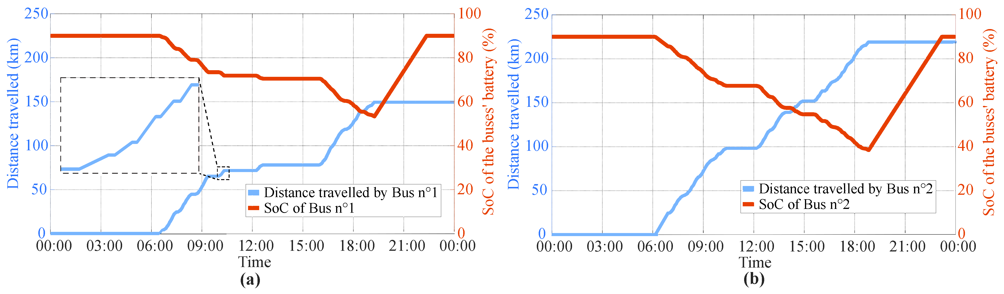
| Consumed energy of bus n°1 (kWh) | 155 | 155 | 140 | 140 | 140 | 140 |
| Consumed energy of bus n°2 (kWh) | 218 | 218 | 197 | 197 | 197 | 197 |
| Minimal SoC of bus n°1 (%) | 53.3 | 79.4 | 45.0 | 44.6 | 65.5 | 69.1 |
| Minimal SoC of bus n°2 (%) | 38.4 | 73.3 | 27.9 | 22.2 | 63.5 | 66.2 |
| Max. total charging power (kW) | 100 | 300 | 350 | 300 | 900 | 1200 |
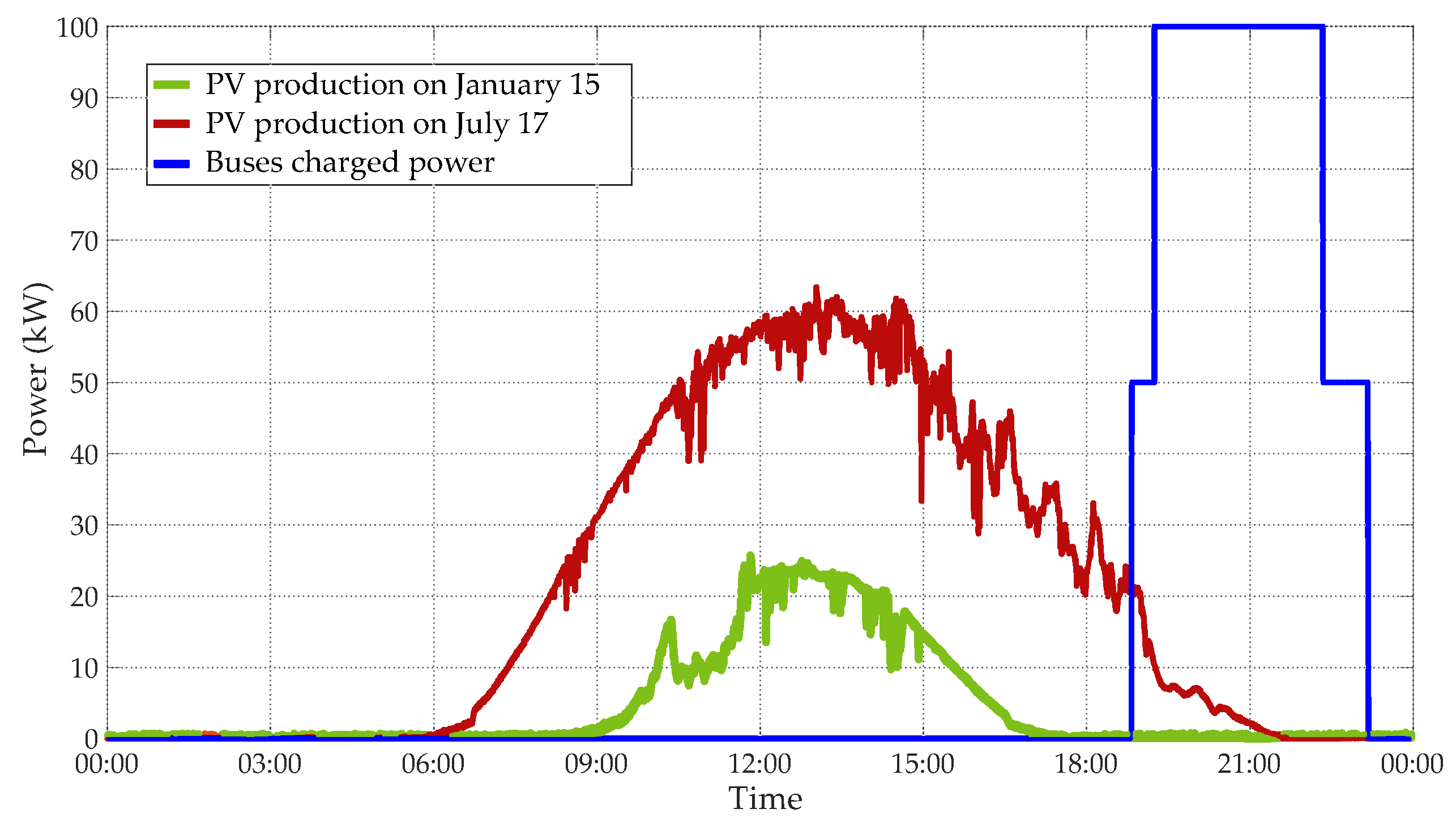
| Influence of PV production on 15 January | ||||||
| PV energy production (kWh) | 108 | 108 | 108 | 108 | 108 | 108 |
| PV energy used for direct charging (kWh) | 1 | 14 | 6 | 13 | 4 | 3 |
| Influence of PV production on 17 July | ||||||
| PV energy production (kWh) | 500 | 500 | 500 | 500 | 500 | 500 |
| PV energy used for direct charging (kWh) | 17 | 81 | 42 | 69 | 24 | 18 |
Disclaimer/Publisher’s Note: The statements, opinions and data contained in all publications are solely those of the individual author(s) and contributor(s) and not of MDPI and/or the editor(s). MDPI and/or the editor(s) disclaim responsibility for any injury to people or property resulting from any ideas, methods, instructions or products referred to in the content. |
© 2023 by the authors. Licensee MDPI, Basel, Switzerland. This article is an open access article distributed under the terms and conditions of the Creative Commons Attribution (CC BY) license (https://creativecommons.org/licenses/by/4.0/).
Share and Cite
Dougier, N.; Celik, B.; Chabi-Sika, S.-K.; Sechilariu, M.; Locment, F.; Emery, J. Modelling of Electric Bus Operation and Charging Process: Potential Contribution of Local Photovoltaic Production. Appl. Sci. 2023, 13, 4372. https://doi.org/10.3390/app13074372
Dougier N, Celik B, Chabi-Sika S-K, Sechilariu M, Locment F, Emery J. Modelling of Electric Bus Operation and Charging Process: Potential Contribution of Local Photovoltaic Production. Applied Sciences. 2023; 13(7):4372. https://doi.org/10.3390/app13074372
Chicago/Turabian StyleDougier, Nathanael, Berk Celik, Salim-Kinnou Chabi-Sika, Manuela Sechilariu, Fabrice Locment, and Justin Emery. 2023. "Modelling of Electric Bus Operation and Charging Process: Potential Contribution of Local Photovoltaic Production" Applied Sciences 13, no. 7: 4372. https://doi.org/10.3390/app13074372