
Analysis of the Influence of Thermal Loading on the Behaviour of the Earth’s Crust


Abstract
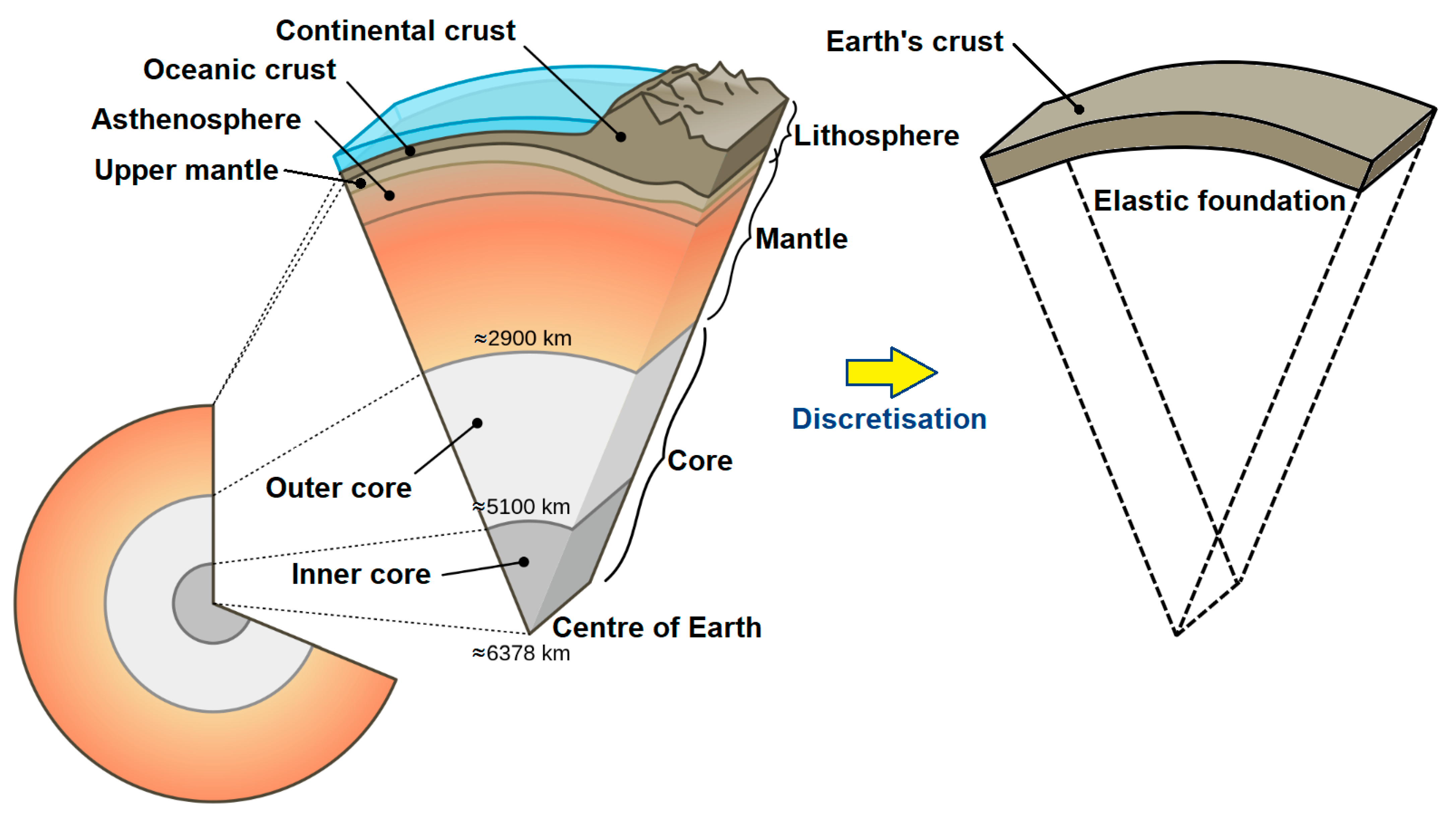
:1. Introduction
2. Materials and Methods
- Young’s modulus E Pa;
- Poisson number μ ∈ ;
- Density (mean value) ρ = 2760 kgm−3;
- Conductivity (thermal conductivity coefficient) λ = 3 Wm−1K−1;
- Specific heat c = 1100 Jkg−1K−1;
- Thermal expansion coefficient α ∈ K−1.
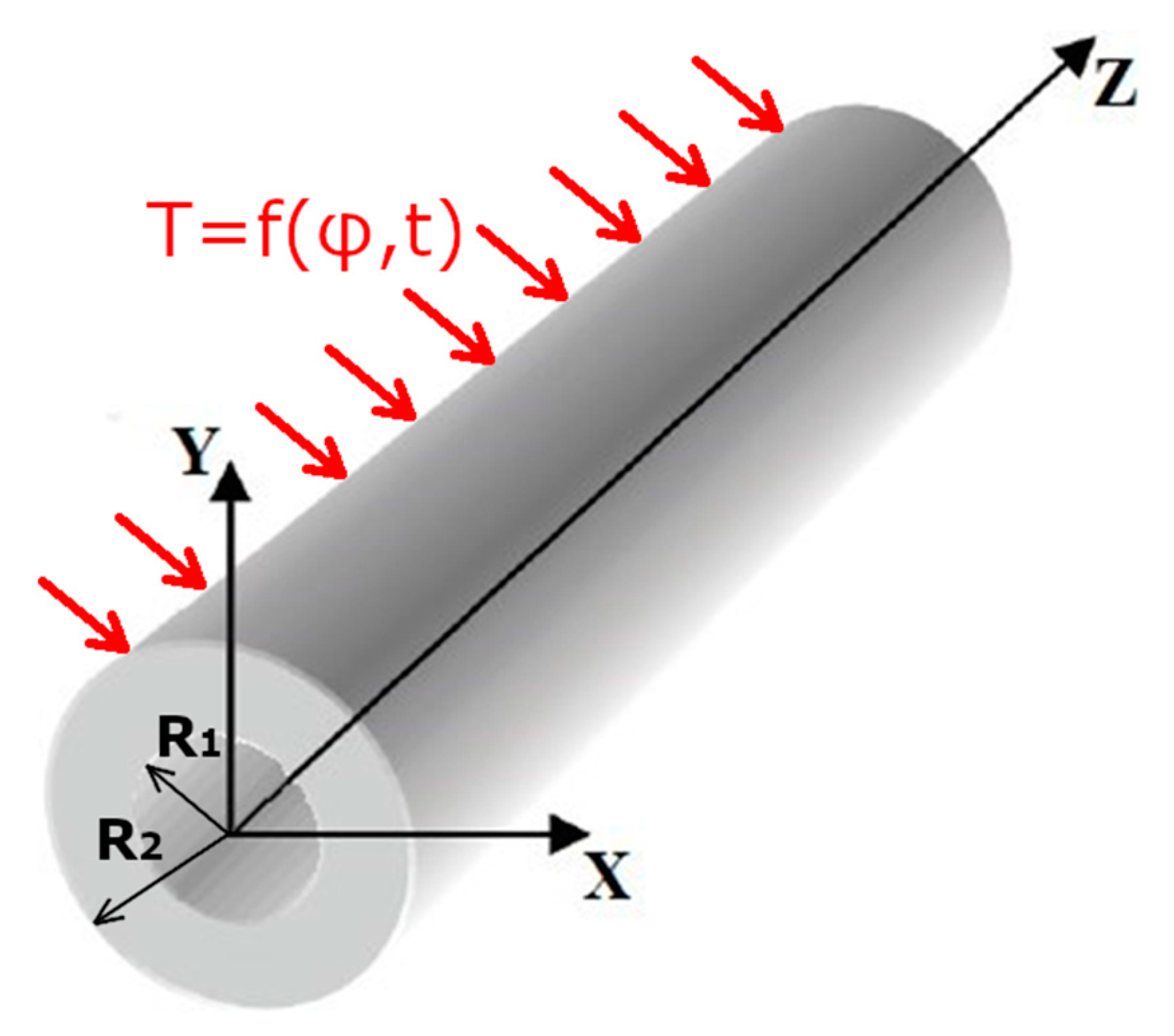
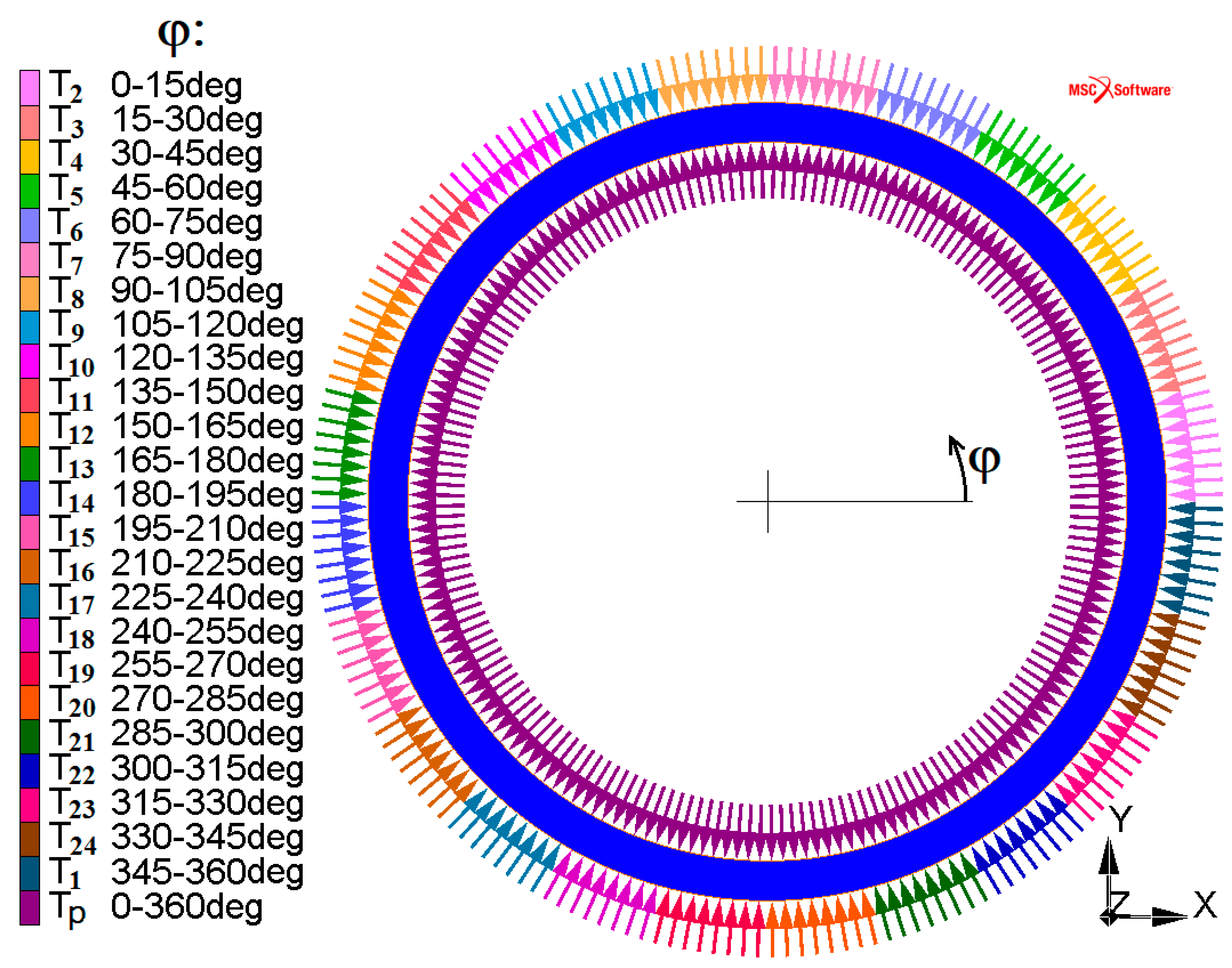
2.1. Temperature Loading
2.1.1. Initial Conditions
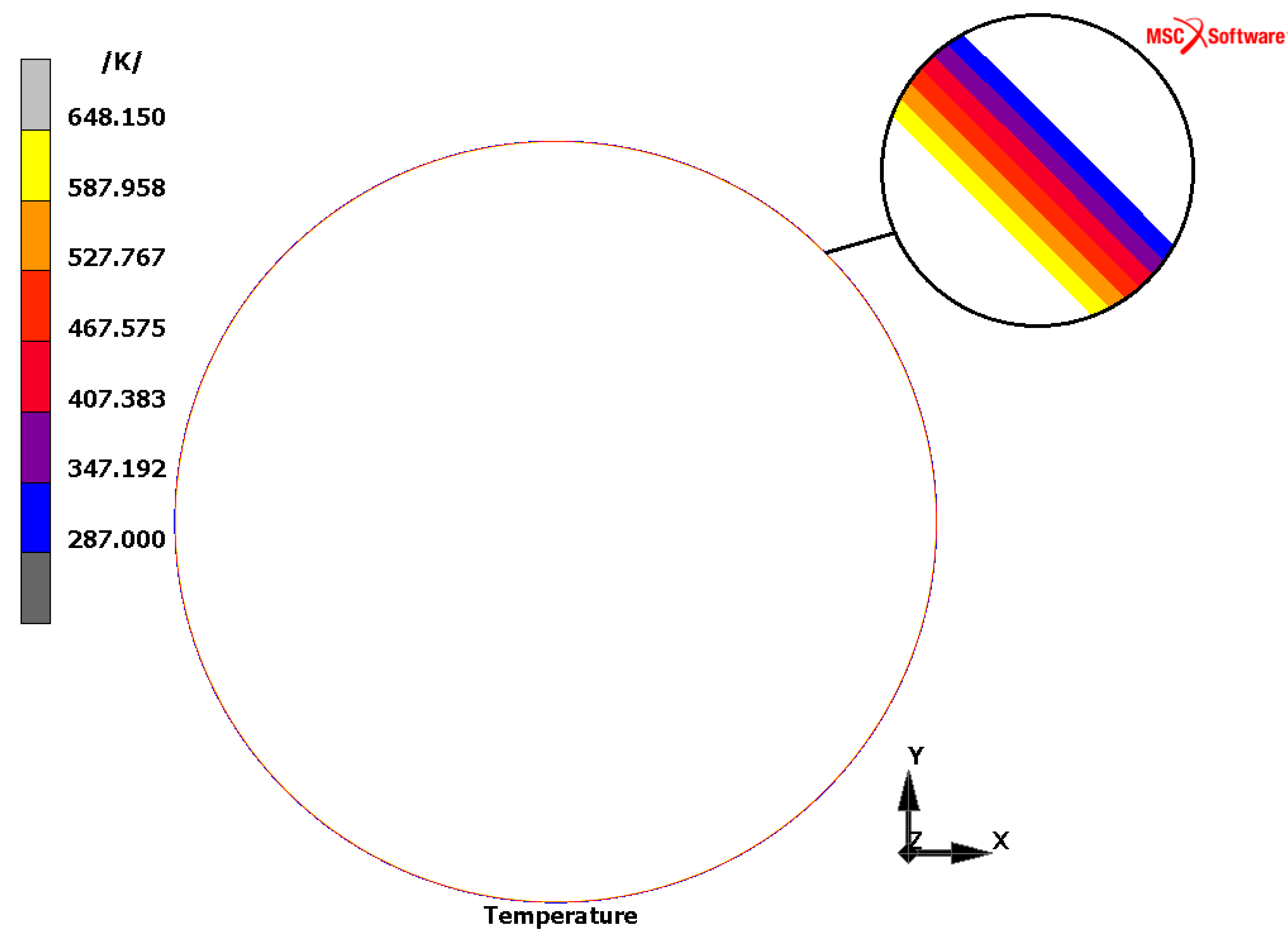
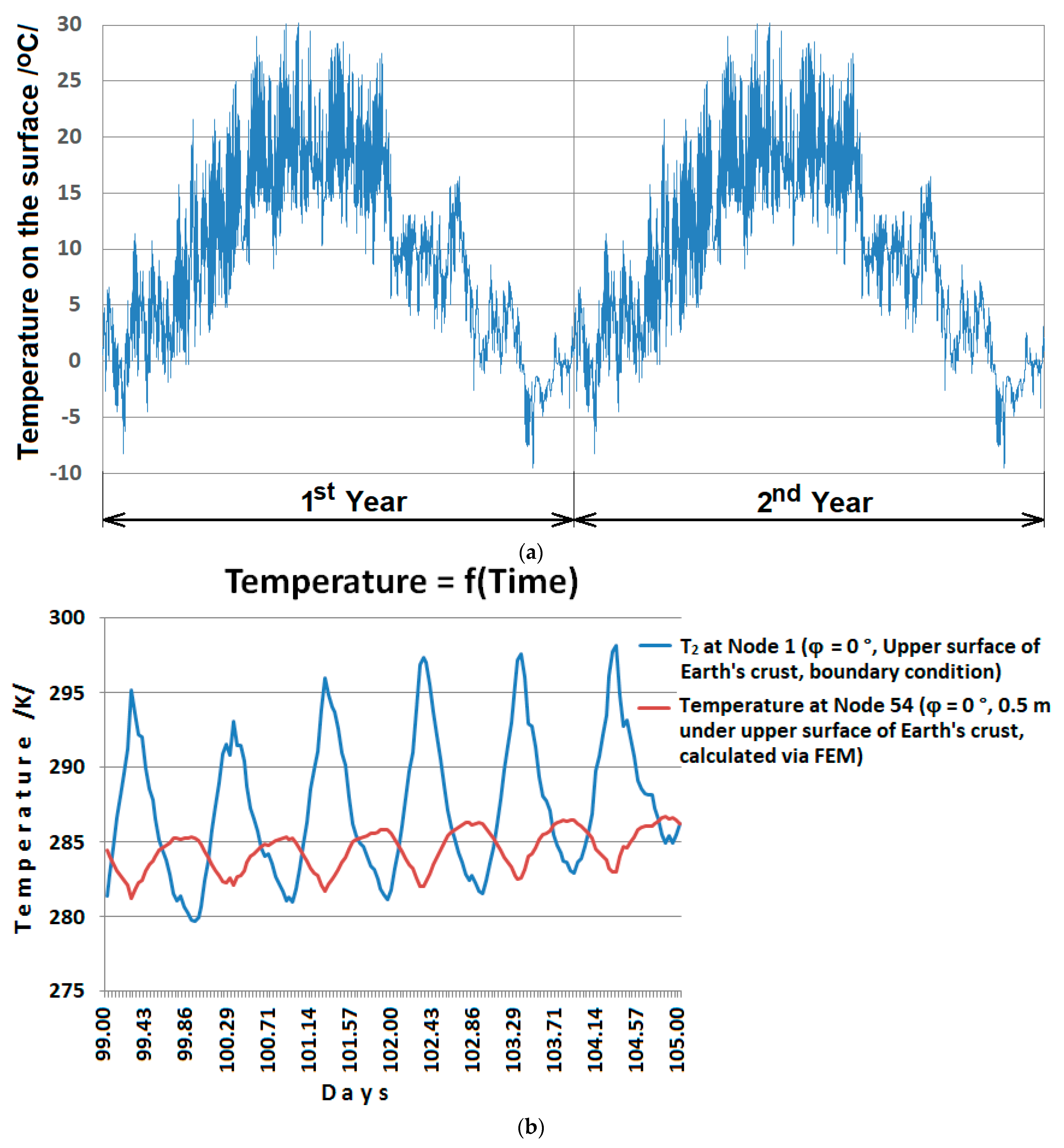
2.1.2. Boundary Conditions
- Minimum temperature = 263.65 K,
- Mean temperature = 282.20 K,
- Median temperature = 282.15 K,
- Standard deviation of temperature = 7.68 K,
- Maximum temperature = 303.35 K.
2.2. Finite Element Mesh
3. Results
3.1. Results from FEA
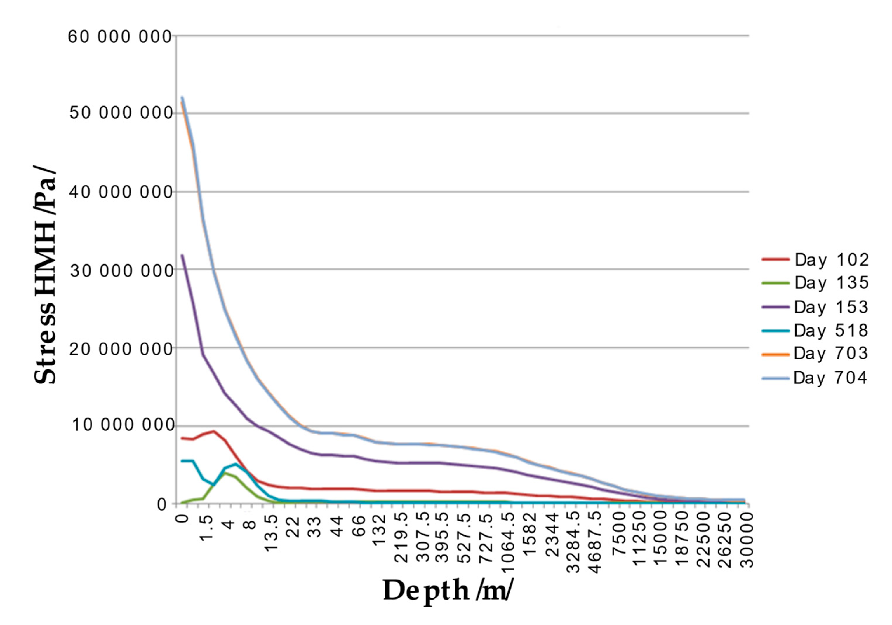
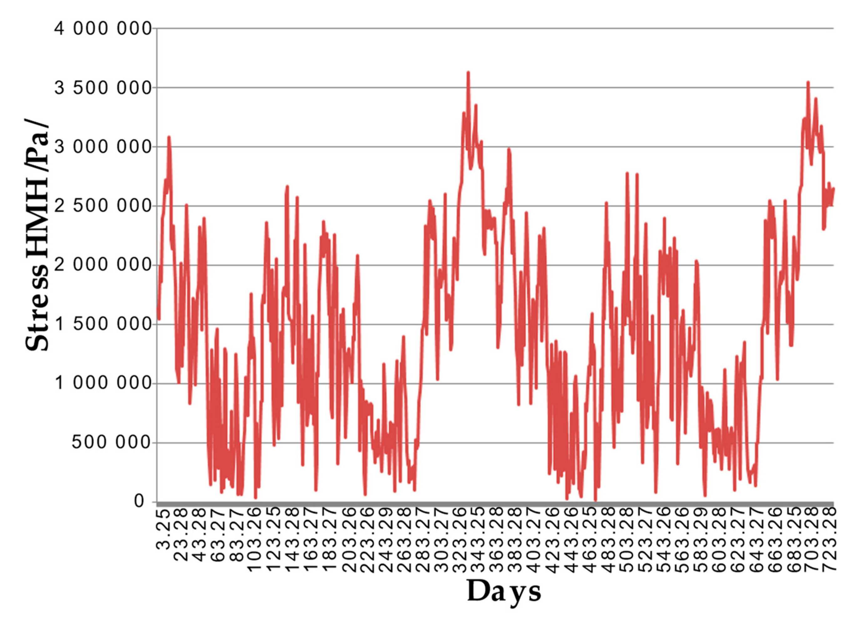
3.1.1. Stress Analysis
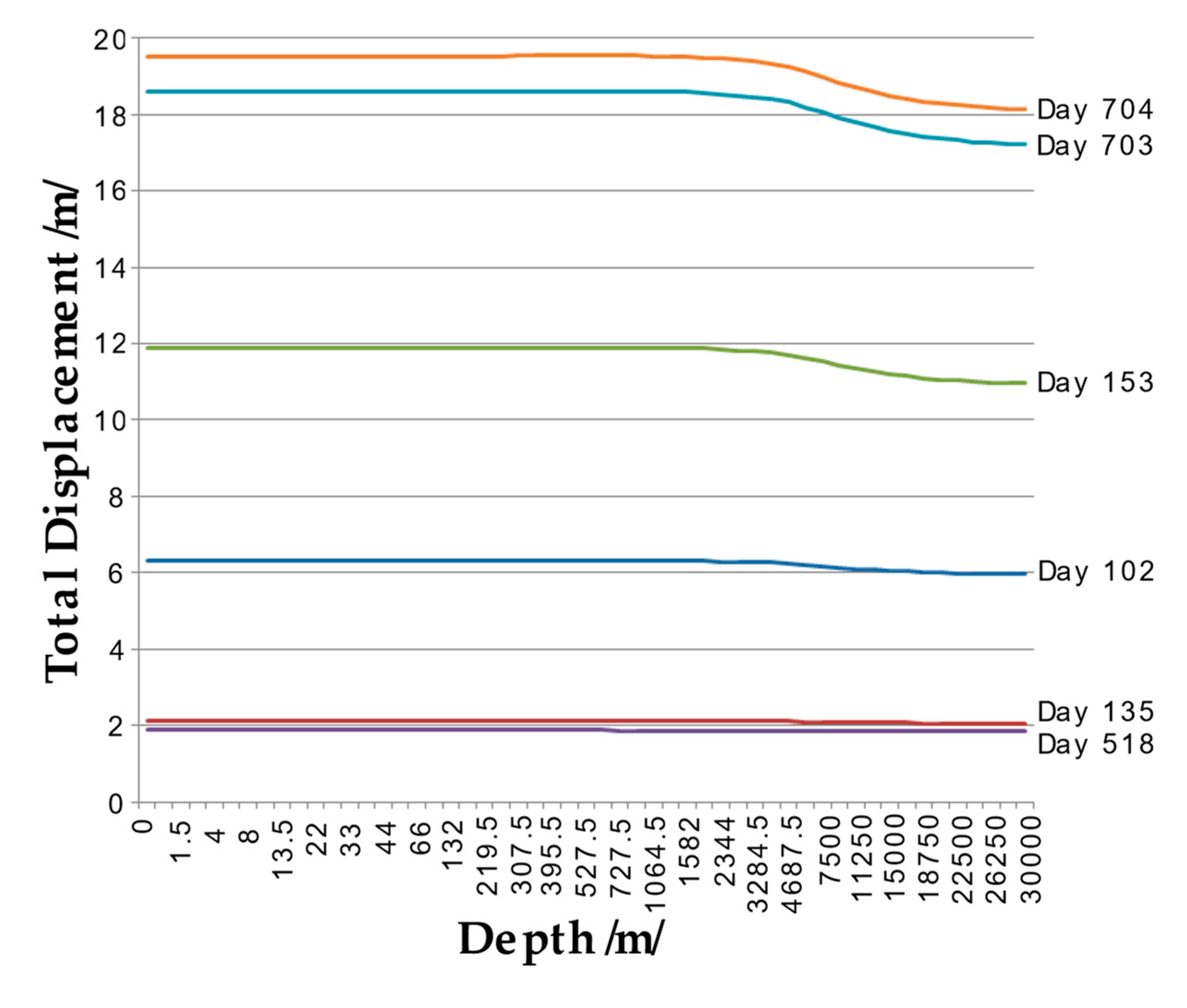
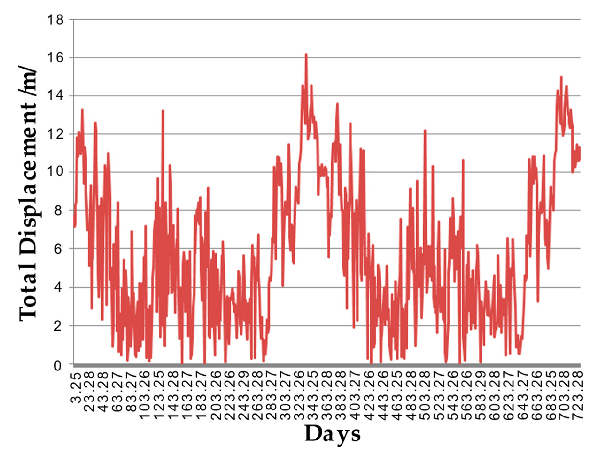
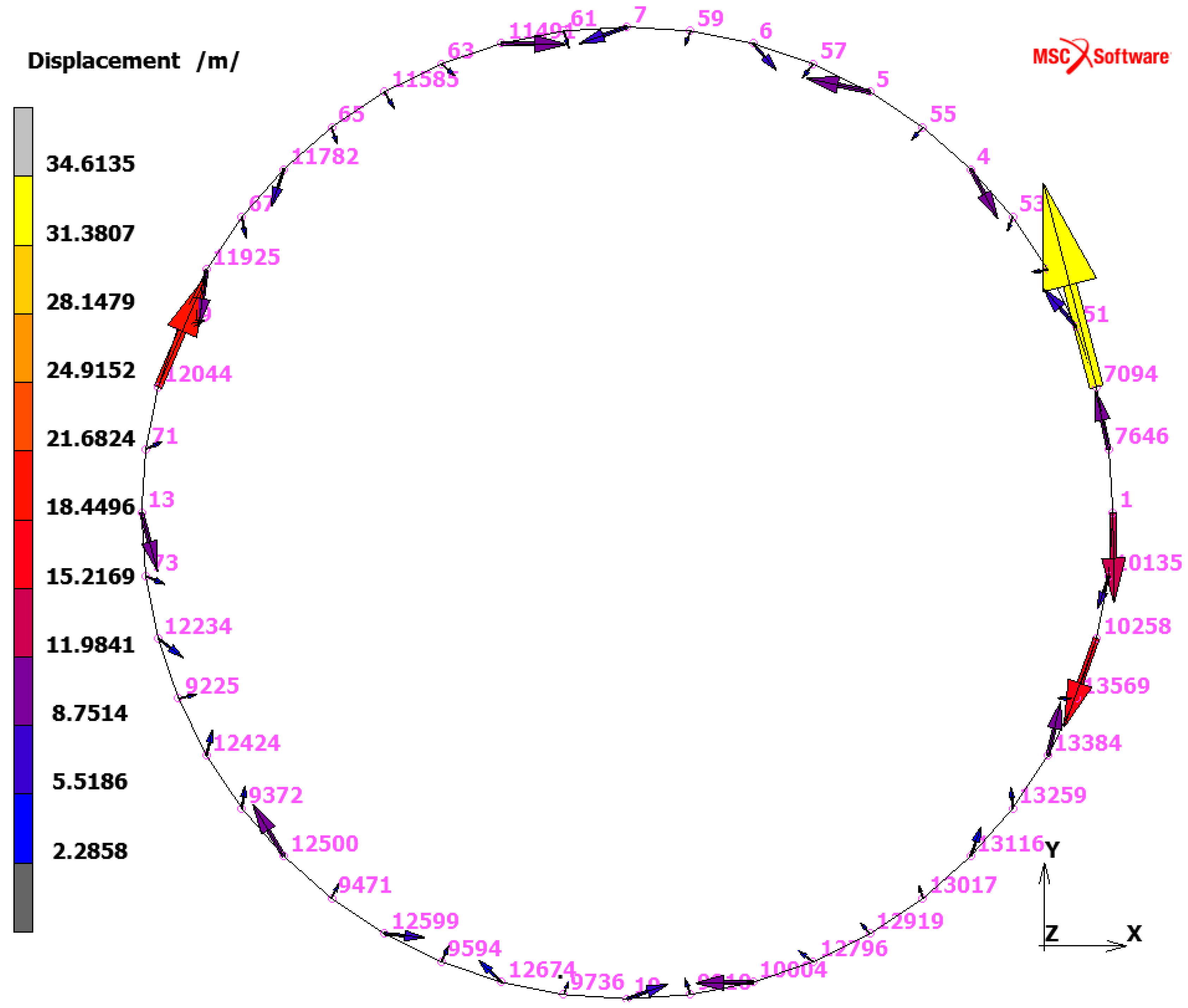
3.1.2. Displacement
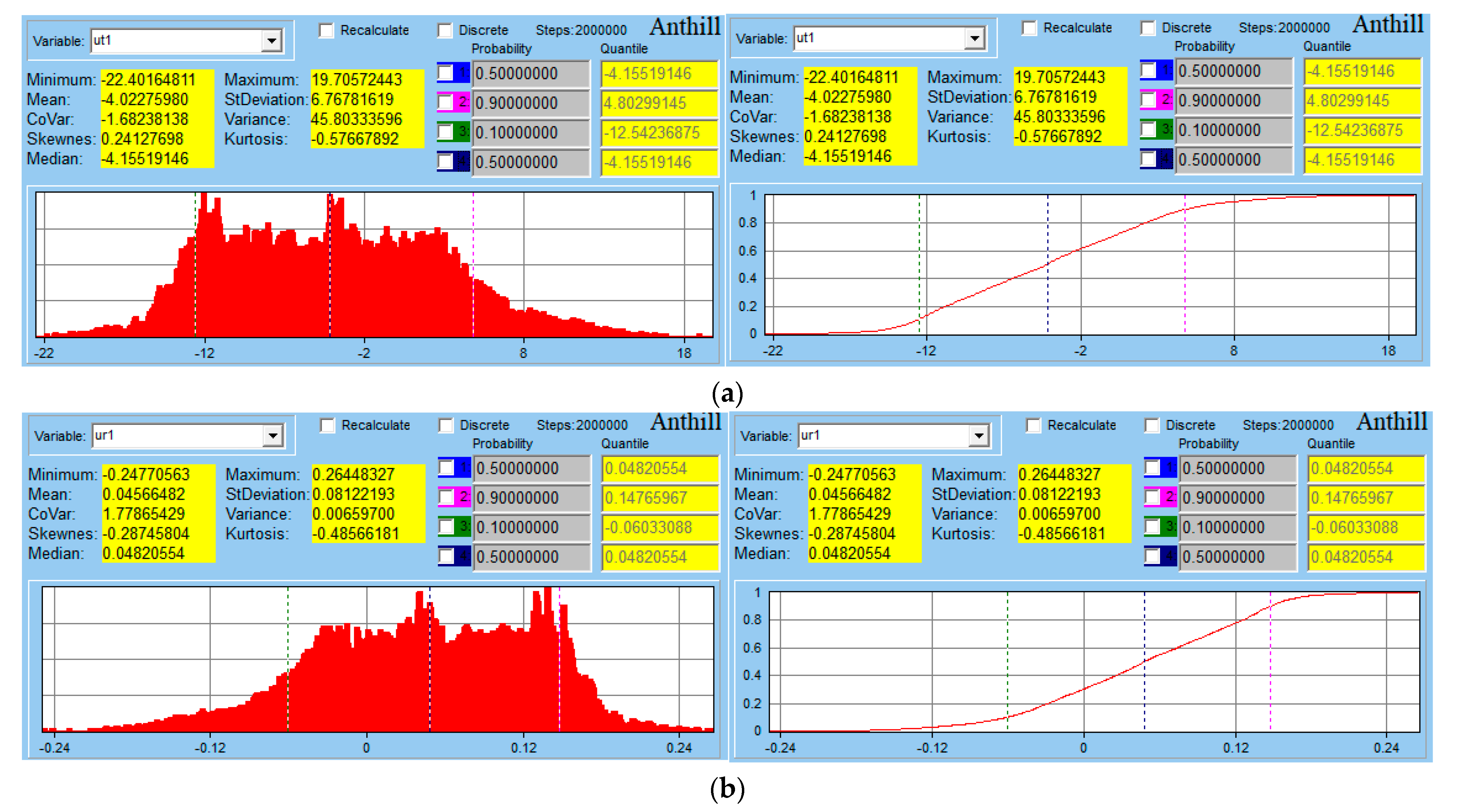
3.2. Stochastic Evaluation of Results
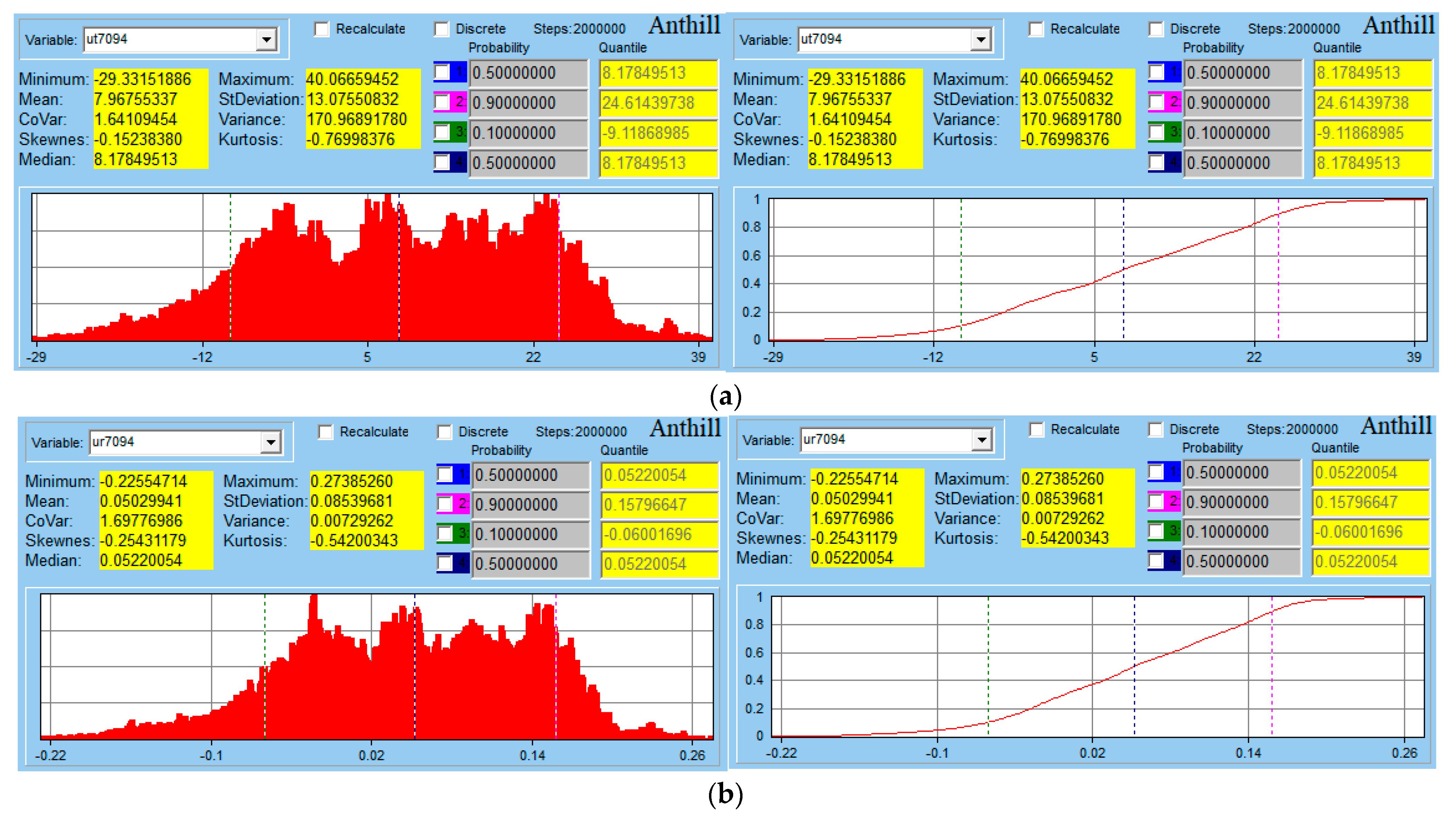
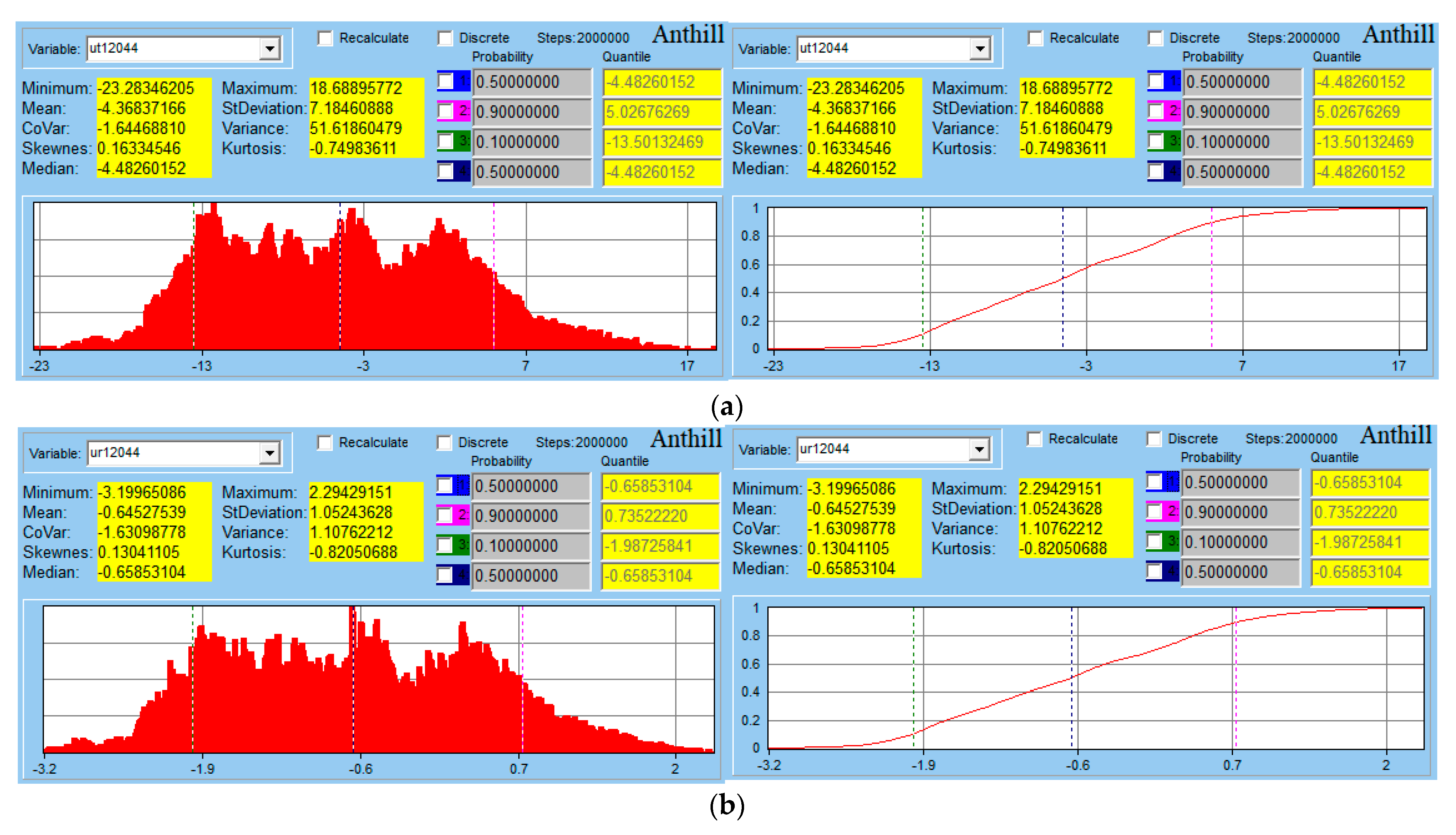
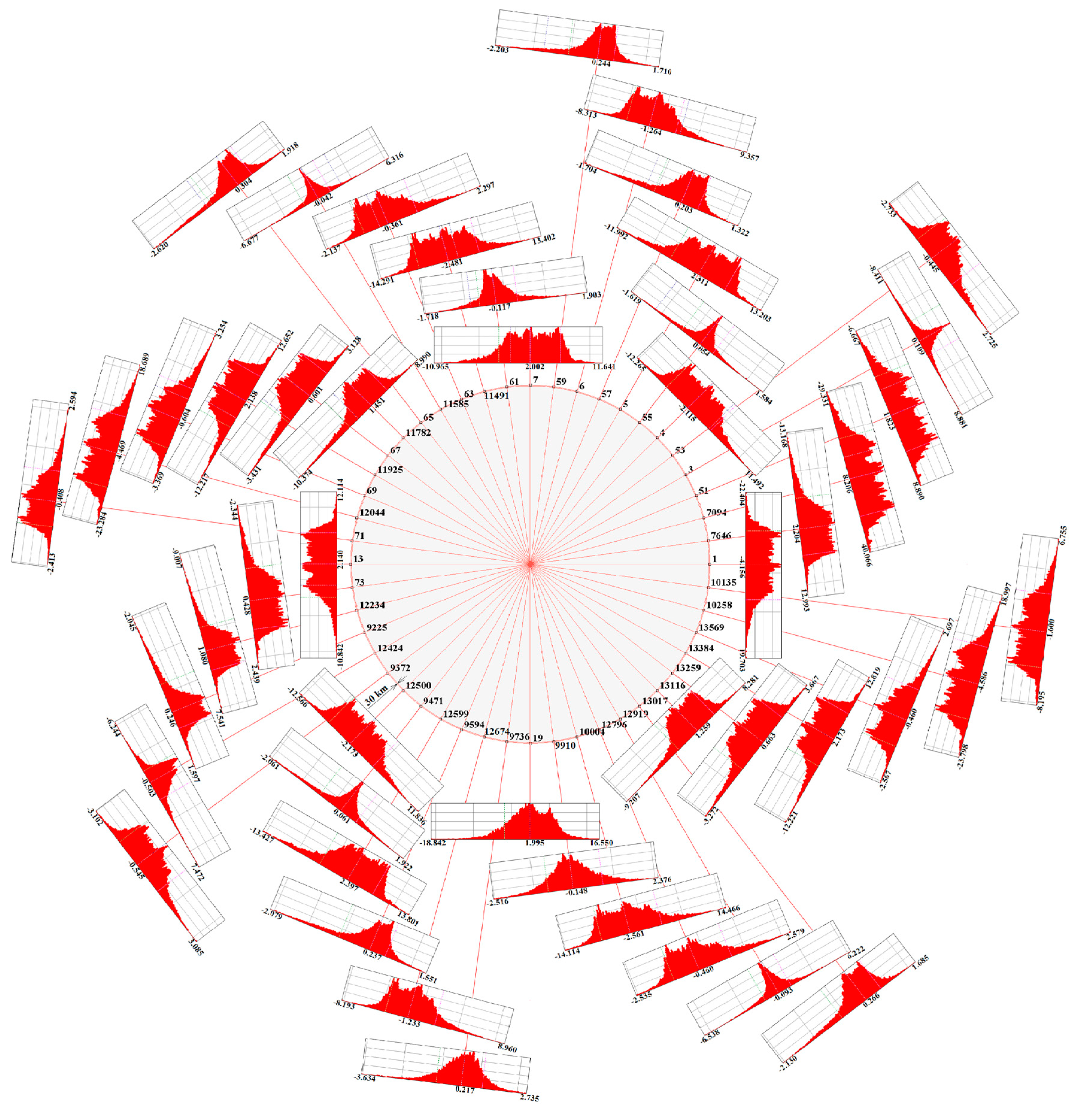
Tangential and Radial Displacement Components
4. Discussion
5. Conclusions
Author Contributions
Funding
Institutional Review Board Statement
Informed Consent Statement
Data Availability Statement
Conflicts of Interest
Nomenclature
| Name | Physical Unit | Explanation |
| ALA | Monitoring system for measuring | |
| c | Jkg−1K−1 | Specific heat of Earth’s crust |
| E | Pa | Young’s modulus of Earth’s crust |
| Earthcylinder | Simplified model of geoid of Earth | |
| 1 | Possible error of Monte Carlo Method | |
| f | Function | |
| FE | Finite element | |
| FEA | Finite Element Analysis | |
| FEM | Finite Element Method | |
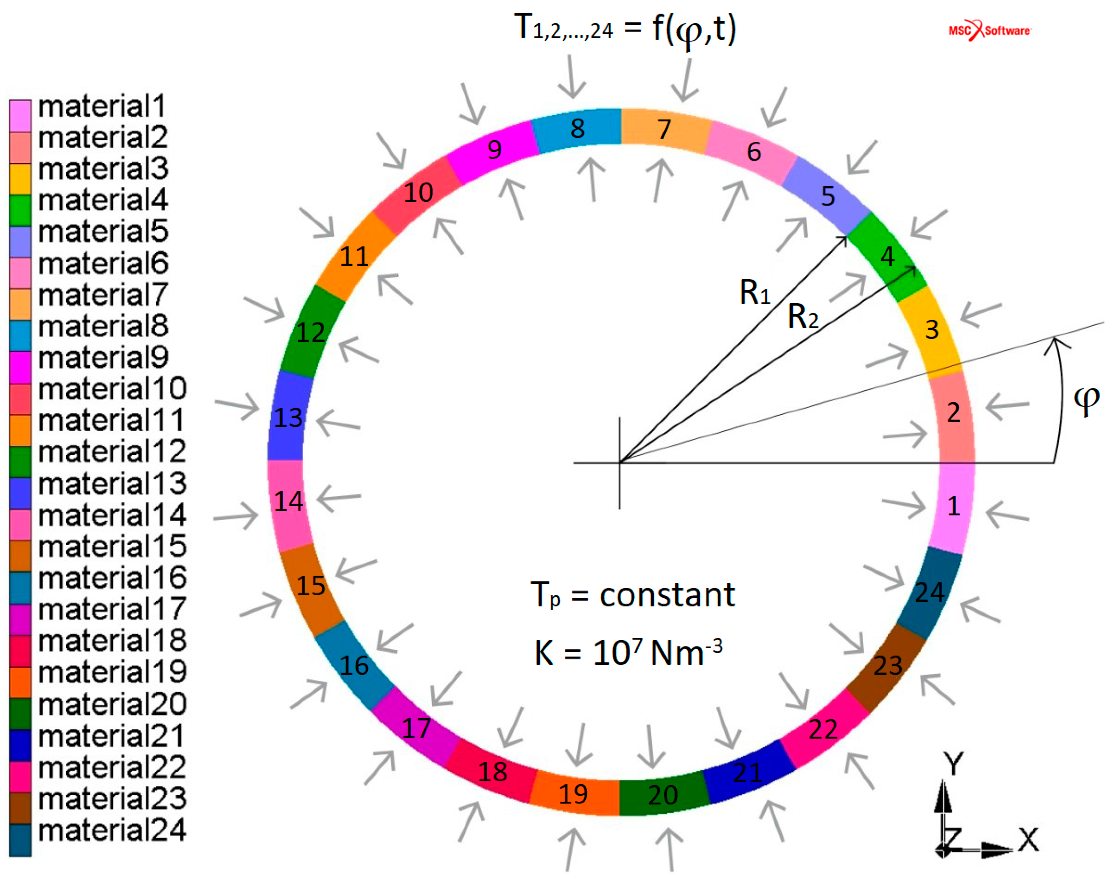
| K | Nm−3 | Modulus of the foundation |
| material1, material2, … material24 | Name of materials in Earth’s crust | |
| Max | Maximum value | |
| Mean | Mean value | |
| Median | Median value | |
| Min | Minimum | |
| MSC.Marc Mentat | Finite element software | |
| Node | Node of finite element mesh | |
| R | m | Radius of Earth’s crust |
| R1 | m | Inner radius of Earth’s crust |
| R2 | m | Outer radius of Earth’s crust |
| Standard deviation | ||
| Number of Monte Carlo simulations | ||
| Stress HMH | Equivalent von Mises stress | |
| T | K | Temperature |
| T1, T2, … T24 | K | Temperature loading on section 1, 2, …, 24 of Earth’s crust, see Figure 3 |
| Tc | K | Initial temperature on inner radius of Earth’s crust, see Figure 5 |
| Tinitial | K | |
| Tp | K | Temperature on inner radius of Earth’s crust |
| t | s | Time |
| m | Total displacement in point of Earth’s crust | |
| m | Tangential component of crustal surface displacement for node 1 | |
| m | Tangential component of crustal surface displacement for node 7094 | |
| m | Tangential component of crustal surface displacement for node 12044 | |
| m | Tangential component of total crustal surface displacement | |
| m | Radial component of crustal surface displacement for node 1 | |
| m | Radial component of crustal surface displacement for node 7094 | |
| m | Radial component of crustal surface displacement for node 12044 | |
| m | Radial component of total crustal surface displacement | |
| m | Displacement in X axis direction | |
| m | Displacement in Y axis direction | |
| X | m | Axis of coordinate system |
| Y | m | Axis of coordinate system |
| Z | m | Axis of coordinate system |
| K−1 | Thermal expansion coefficient of Earth’s crust | |
| deg | Angle of Earth’s crust | |
| Wm−1K−1 | Conductivity of Earth’s crust | |
| μ | 1 | Poisson number of Earth’s crust |
| ρ | Kgm−3 | Density of Earth’s crust |
| Pa | Equivalent von Mises Stress | |
| Pa | Principal stress |
References
- Available online: https://commons.wikimedia.org/wiki/File:Earth_and_its_simplification.png (accessed on 31 January 2023).
- Ammon, C.J.; Velasco, A.A.; Lay, T.; Wallace, T.C. Foundations of Modern Global Seismology, 2nd ed.; Academic Press: Cambridge, MA, USA; Elsevier Inc.: Amsterdam, The Netherlands, 2021; ISBN 978-0-12-815679-7. [Google Scholar]
- Gupta, H.; Roy, S. Geothermal Energy, an Alternative Resource for the 21st Century; Elsevier: Amsterdam, The Netherlands, 2007. [Google Scholar] [CrossRef]
- Fei, H.; Yamazaki, D.; Sakurai, M.; Miyajima, N.; Ohfuji, H.; Katsura, T.; Yamamoto, T. A Nearly Water-Saturated Mantle Transition Zone Inferred from Mineral Viscosity. Sci. Adv. 2017, 3, e1603024. [Google Scholar] [CrossRef] [PubMed] [Green Version]
- Ohtani, E. The Role of Water in Earth’s Mantle. Natl. Sci. Rev. 2020, 7, 224–232. [Google Scholar] [CrossRef] [PubMed]
- Zang, A.; Stephansson, O. Stress Field of the Earth’s Crust; Springer Science & Business Media: Berlin/Heidelberg, Germany, 2009. [Google Scholar] [CrossRef]
- Stracke, A. Composition of Earth’s Mantle. In Encyclopedia of Geology, 2nd ed.; Alderton, D., Elias, S.A., Eds.; Academic Press: Cambridge, MA, USA, 2021; pp. 164–177. [Google Scholar] [CrossRef]
- Mahatsente, R.; Ranalli, G.; Bolte, D.; Götze, H.-J. On the relation between lithospheric strength and ridge push transmission in the Nazca plate. J. Geodyn. 2012, 53, 18–26. [Google Scholar] [CrossRef]
- Wandrol, I. Modelling of Mechanical Behavior of the Earth’s Crust. Ph.D. Dissertation, Department of Applied Mechanics, Faculty of Mechanical Engineering, VŠB-TU Ostrava, Ostrava, Czech Republic, 2007. (In Czech). [Google Scholar]
- Monitoring system ALA. Web Page, Results of Surface Temperature Measurement with the System ALA. 2017. Available online: http://teranos.ala1.com/en/indexc.php (accessed on 16 June 2017).
- Available online: http://teranos.ala1.com/en/info.php (accessed on 31 January 2023).
- Mingming, L.; McNamara, A.K. Evolving morphology of crustal accumulations in Earth’s lowermost mantle. Earth Planet. Sci. Lett. 2022, 577, 117265. [Google Scholar] [CrossRef]
- Frydrýšek, K. Nosníky a Rámy na Pružném Podkladu 1 (Beams and Frames on Elastic Foundation); VSB—Technical University of Ostrava, Faculty of Mechanical Engineering: Ostrava, Czech Republic, 2006; pp. 1–463. ISBN 80-248-1244-4. [Google Scholar]
- Frydrýšek, K. Nosníky a Rámy na Pružném Podkladu 2 (Beams and Frames on Elastic Foundation 2); VSB—Technical University of Ostrava, Faculty of Mechanical Engineering: Ostrava, Czech Republic, 2008; pp. 1–516. ISBN 978-80-248-1743-9. [Google Scholar]
- Frydrýšek, K. Beams and Frames on Elastic Foundation 3; VSB—Technical University of Ostrava, Faculty of Mechanical Engineering: Ostrava, Czech Republic, 2010; ISBN 978-80-248-2257-0. [Google Scholar]
- Tvrdá, K. Probability and Sensitivity Analysis of Plate. Applied Mechanics and Materials; Trans Tech Publications Ltd.: Zurich, Switzerland, 2014; Volume 617, pp. 193–196. [Google Scholar]
- Čajka, R.; Vašková, J.; Vašek, J. Numerical Analyses of Subsoil-structure Interaction in Original Non-commercial Software based on FEM. IOP Conf. Ser. Earth Environ. Sci. 2018, 143, 012003. [Google Scholar] [CrossRef]
- Wandrol, I.; Frydrýšek, K.; Hofer, A. Surface Temperature Model—Analysis of Earth’s Crust Response to Changes in Surface Temperature. In Proceedings of the Engineering Mechanics 2019—25th International Conference, Svratka, Czech Republic, 13–16 May 2019; pp. 399–402. [Google Scholar] [CrossRef] [Green Version]
- Wandrol, I.; Frydrýšek, K.; Kalenda, P. About the SBRA Method Applied in Mechanics of Continental Plates. Trans. VŠB—Tech. Univ. Ostrava 2013, LIX, 143–150. [Google Scholar] [CrossRef] [PubMed]
- Famfulík, J.; Míková, J.; Lánská, M.; Richtář, M. A Stochastic Model of the Logistics Actions Required to Ensure the Availability of Spare Parts During Maintenance of Railway Vehicles. Proc. Inst. Mech. Eng. Part F J. Rail Rapid Transit 2014, 228, 85–92. [Google Scholar] [CrossRef]
- Vavrušová, K.; Mikolášek, D.; Lokaj, A.; Klajmonová, K.; Sucharda, O.; Parenica, P. Determination of Carrying Capacity of Steel-Timber Joints with Steel Rods Glued-In Parallel to Grain. Wood Res. 2016, 61, 733–740. [Google Scholar]
- Maléřová, L.; Pokorný, J.; Kristlová, E.; Wojnarova, J. Using of mobile flood protection on the territory of the Moldova as possible protection of the community. IOP Conf. Ser. Earth Environ. Sci. 2017, 92, 12039. [Google Scholar] [CrossRef] [Green Version]
- Abbaszadeh Shahri, A.; Shan, C.; Larsson, S. A Novel Approach to Uncertainty Quantification in Groundwater Table Modeling by Automated Predictive Deep Learning. Nat. Resour. Res. 2022, 31, 1351–1373. [Google Scholar] [CrossRef]
- Frydrýšek, K.; Václavek, L. Stochastic computer approach applied in the reliability assessment of engineering structures. In Proceedings of the First International Scientific Conference “Intelligent Information Technologies for Industry” (IITI’16), Rostov-on-Don, Russia, 16–21 May 2016; Springer: Cham, Switzerland, 2016. [Google Scholar] [CrossRef]
- Kesl, P.; Plánička, F. Possibility of application of the simulation based assessment method in modelling of structures. EUT Edizioni Università di Trieste. In Proceedings of the 34th Danubia-Adria Symposium on Advances in Experimental Mechanics, Trieste, Italy, 19–22 September 2017. [Google Scholar]
- Kalenda, P.; Wandrol, I.; Holub, K.; Rušajová, J. The possible explanation for secondary microseisms seasonal and annual variations. Terr. Atmos. Ocean. Sci. 2015, 26, 103–109. [Google Scholar] [CrossRef] [Green Version]
- Frydrýšek, K.; Šír, M.; Pleva, L.; Szeliga, J.; Stránský, J.; Čepica, D.; Kratochvíl, J.; Koutecký, J.; Madeja, R.; Dědková, K.P. Stochastic Strength Analyses of Screws for Femoral Neck Fractures. Appl. Sci. 2022, 12, 1015. [Google Scholar] [CrossRef]
- Berger, J. A note on thermoelastic strains and tilts. J. Geophys. Res. 1975, 80, 274–277. [Google Scholar] [CrossRef]
- Croll, J.G.A. Mechanics of thermal ratchet uplift buckling in periglacial morphologies. In Proceedings of the SEMC Conference, Cape Town, South Africa, 10–12 September 2007. [Google Scholar]
- Kalenda, P.; Neuman, L.; Málek, J.; Skalský, L.; Procházka, V.; Ostříhanský, L.; Kopf, T.; Wandrol, I. Tilts, Global Tectonics and Earthquake Prediction; SWB: London, UK, 2012; pp. 1–247. [Google Scholar]
- Frydrýšek, K.; Wandrol, I.; Kalenda, P. Report about the Probabilistic Approaches Applied in Mechanics of Continental Plates. Math. Models Methods Mod. Sci. 2012, 3, 146–149. [Google Scholar]
- Abbaszadeh Shahri, A.; Kheiri, A.; Hamzeh, A. Subsurface Topographic Modeling Using Geospatial and Data Driven Algorithm. ISPRS Int. J. Geo-Inf. 2021, 10, 341. [Google Scholar] [CrossRef]
- Miyazaki, Y.; Korenaga, J. On the timescale of magma ocean solidification and its chemical consequences: 2. Compositional differentiation under crystal accumulation and matrix compaction. J. Geophys. Res. Solid Earth 2019, 124, 3399–3419. [Google Scholar] [CrossRef]
- Tschauner, O.; Huang, S.; Greenberg, E.; Prakapenka, V.B.; Ma, C.; Rossman, G.R.; Shen, A.H.; Zhang, D.; Newville, M.; Lanzirotti, A.; et al. Ice-VII inclusions in diamonds: Evidence for aqueous fluid in Earth’s deep mantle. Science 2018, 359, 1136–1139. [Google Scholar] [CrossRef] [PubMed] [Green Version]
- Shen, J.H.; Wang, X.; Cui, J.; Wang, X.Z.; Zhu, C.Q. Study on the shear characteristics of calcareous gravelly sand considering particle breakage. Bull. Eng. Geol. Environ. 2022, 81, 130. [Google Scholar] [CrossRef]
- Peslier, A.H.; Schönbächler, M.; Busemann, H.; Karato, S.-I. Water in the Earth’s Interior: Distribution and Origin. Space Sci. Rev. 2017, 212, 743–810. [Google Scholar] [CrossRef]
- Bonchkovskii, V.F. Vnutrennee Stroenie Zemli; Akademii nauk SSSR: Moscow, Russia, 1953; pp. 1–173. (In Russian) [Google Scholar]
- Čermák, V. Coefficient of thermal conductivity of some sediments and its dependence on density and water content of rocks. Chemie Erde. 1967, 26, 271–278. [Google Scholar]
- Mareš, S. Úvod do Užité Geofyziky: Vysokoškolská Učebnice; Státní nakladatelství technické literatury: Prague, Czech Republic, 1979; pp. 1–590. (In Czech) [Google Scholar]
- Quali, S. Thermal Conductivity in Relation to Porosity and Geological Stratigraphy; Geothermal Training Programme; United Nations University: Reykjavík, Iceland, 2009; Volume 23, pp. 495–512. Available online: http://www.os.is/gogn/unu-gtp-report/UNU-GTP-2009-23.pdf (accessed on 28 March 2023).
- Beazly, M. Anatomie Země; Albatros: Prague, Czech Republic, 1981; pp. 1–121. (In Czech) [Google Scholar]
- MSC Software, MSC. Marc Mentat [Computer Software]. Available online: https://www.mscsoftware.com/product/marc (accessed on 31 January 2023).
- Available online: https://en.wikipedia.org/wiki/Von_Mises_yield_criterion (accessed on 31 January 2023).
- Guštar, M.; Marek, P. Anthill (Version 2.6 Pro) [Computer Software]. Available online: http://www.noise.cz/sbra/software.html (accessed on 31 January 2023).
- Marek, P.; Brozzetti, J.; Guštar, M. Probabilistic Assessment of Structures Using Monte Carlo Simulation: Background, Exercises and Software, 2nd ed.; Institute of Theoretical and Applied Mechanics, Academy of Sciences of the Czech Republic: Prague, Czech Republic, 2003. [Google Scholar]
- Available online: https://web.northeastern.edu/afeiguin/phys5870/phys5870/node71.html (accessed on 31 January 2023).


| Section | Angle ϕ /deg/ | Young’s Modulus E/Pa/ | Poisson Number /1/ | Density /kg∙m−3/ | Conductivity /W∙m−1∙K−1/ | Specific Heat /J∙K−1∙kg−1/ | Thermal Expansion /K−1/ |
|---|---|---|---|---|---|---|---|
| 1 | 345–360 | 3.00 × 10¹⁰ | 0.30 | 2760 | 3 | 1100 | 3.50 × 10⁻⁵ |
| 2 | 0–15 | 3.50 × 10¹⁰ | 0.35 | 2760 | 3 | 1100 | 4.00 × 10⁻⁵ |
| 3 | 15–30 | 4.00 × 10¹⁰ | 0.30 | 2760 | 3 | 1100 | 4.50 × 10⁻⁵ |
| 4 | 30–45 | 4.50 × 10¹⁰ | 0.35 | 2760 | 3 | 1100 | 3.50 × 10⁻⁵ |
| 5 | 45–60 | 3.00 × 10¹⁰ | 0.30 | 2760 | 3 | 1100 | 4.00 × 10⁻⁵ |
| 6 | 60–75 | 3.50 × 10¹⁰ | 0.35 | 2760 | 3 | 1100 | 4.50 × 10⁻⁵ |
| 7 | 75–90 | 4.00 × 10¹⁰ | 0.30 | 2760 | 3 | 1100 | 3.50 × 10⁻⁵ |
| 8 | 90–105 | 4.50 × 10¹⁰ | 0.35 | 2760 | 3 | 1100 | 4.00 × 10⁻⁵ |
| 9 | 105–120 | 3.00 × 10¹⁰ | 0.30 | 2760 | 3 | 1100 | 4.50 × 10⁻⁵ |
| 10 | 120–135 | 3.50 × 10¹⁰ | 0.35 | 2760 | 3 | 1100 | 3.50 × 10⁻⁵ |
| 11 | 135–150 | 4.00 × 10¹⁰ | 0.30 | 2760 | 3 | 1100 | 4.00 × 10⁻⁵ |
| 12 | 150–165 | 4.50 × 10¹⁰ | 0.35 | 2760 | 3 | 1100 | 4.50 × 10⁻⁵ |
| 13 | 165–180 | 3.00 × 10¹⁰ | 0.30 | 2760 | 3 | 1100 | 3.50 × 10⁻⁵ |
| 14 | 180–195 | 3.50 × 10¹⁰ | 0.35 | 2760 | 3 | 1100 | 4.00 × 10⁻⁵ |
| 15 | 195–210 | 4.00 × 10¹⁰ | 0.30 | 2760 | 3 | 1100 | 4.50 × 10⁻⁵ |
| 16 | 210–225 | 4.50 × 10¹⁰ | 0.35 | 2760 | 3 | 1100 | 3.50 × 10⁻⁵ |
| 17 | 225–240 | 3.00 × 10¹⁰ | 0.30 | 2760 | 3 | 1100 | 4.00 × 10⁻⁵ |
| 18 | 240–255 | 3.50 × 10¹⁰ | 0.35 | 2760 | 3 | 1100 | 4.50 × 10⁻⁵ |
| 19 | 255–270 | 4.00 × 10¹⁰ | 0.30 | 2760 | 3 | 1100 | 3.50 × 10⁻⁵ |
| 20 | 270–285 | 4.50 × 10¹⁰ | 0.35 | 2760 | 3 | 1100 | 4.00 × 10⁻⁵ |
| 21 | 285–300 | 3.00 × 10¹⁰ | 0.30 | 2760 | 3 | 1100 | 4.50 × 10⁻⁵ |
| 22 | 300–315 | 3.50 × 10¹⁰ | 0.35 | 2760 | 3 | 1100 | 3.50 × 10⁻⁵ |
| 23 | 315–330 | 4.00 × 10¹⁰ | 0.30 | 2760 | 3 | 1100 | 4.00 × 10⁻⁵ |
| 24 | 330–345 | 4.50 × 10¹⁰ | 0.35 | 2760 | 3 | 1100 | 4.50 × 10⁻⁵ |
| Node | Angle ϕ /deg/ | Min /m/ | Mean /m/ | Median /m/ | Max /m/ |
|---|---|---|---|---|---|
| 1 | 0.0 | −22.405145 | −4.016917 | −4.155867 | 19.706385 |
| 7646 | 7.5 | −13.167980 | 1.980264 | 2.203522 | 12.992962 |
| 7094 | 15.0 | −29.331777 | 7.971764 | 8.205548 | 40.070023 |
| 51 | 22.5 | −6.667464 | 1.772484 | 1.822645 | 8.890464 |
| 3 | 30.0 | −8.410809 | 0.015862 | 0.108814 | 8.880879 |
| 53 | 37.5 | −2.733061 | −0.369284 | −0.444654 | 2.724747 |
| 4 | 45.0 | −12.265832 | −2.029589 | −2.114735 | 11.494079 |
| 55 | 52.5 | −1.619803 | 0.019862 | 0.053834 | 1.584367 |
| 5 | 60.0 | −11.991985 | 2.225961 | 2.311249 | 13.202844 |
| 57 | 67.5 | −1.703642 | 0.148204 | 0.202752 | 1.321986 |
| 6 | 75.0 | −8.316151 | −1.156488 | −1.263755 | 9.357056 |
| 59 | 82.5 | −2.202902 | 0.168749 | 0.243539 | 1.710141 |
| 7 | 90.0 | −10.964751 | 1.914396 | 2.002252 | 11.641080 |
| 61 | 97.5 | −1.717808 | −0.088355 | −0.117302 | 1.903794 |
| 11491 | 105.0 | −14.292981 | −2.386571 | −2.480774 | 13.402903 |
| 63 | 112.5 | −2.136792 | −0.321966 | −0.361097 | 2.297582 |
| 11585 | 120.0 | −6.676715 | −0.051041 | −0.041540 | 6.316006 |
| 65 | 127.5 | −2.620005 | 0.196727 | 0.304310 | 1.918440 |
| 11782 | 135.0 | −10.374590 | 1.212906 | 1.450878 | 8.992166 |
| 67 | 142.5 | −3.431526 | 0.537606 | 0.601411 | 3.128304 |
| 11925 | 150.0 | −12.217613 | 2.033221 | 2.138069 | 12.652762 |
| 69 | 157.5 | −3.368985 | −0.578049 | −0.604307 | 3.254372 |
| 12044 | 165.0 | −23.284528 | −4.365703 | −4.469298 | 18.689545 |
| 71 | 172.5 | −2.412931 | −0.367422 | −0.407727 | 2.594586 |
| 13 | 180.0 | −10.843711 | 2.072278 | 2.139710 | 12.114409 |
| 73 | 187.5 | −2.344523 | 0.396470 | 0.427631 | 2.438536 |
| 12234 | 195.0 | −9.007515 | 0.961226 | 1.080069 | 7.542674 |
| 9225 | 202.5 | −2.045828 | 0.180401 | 0.245550 | 1.597627 |
| 12424 | 210.0 | −6.245059 | −0.379791 | −0.502522 | 7.471727 |
| 9372 | 217.5 | −3.101930 | −0.514486 | −0.545275 | 3.085332 |
| 12500 | 225.0 | −12.566509 | −2.093027 | −2.173286 | 11.838935 |
| 9471 | 232.5 | −2.061168 | 0.018279 | 0.060519 | 1.922392 |
| 12599 | 240.0 | −13.427477 | 2.207517 | 2.396578 | 13.803798 |
| 9594 | 247.5 | −2.078801 | 0.147412 | 0.237499 | 1.551424 |
| 12674 | 255.0 | −8.193241 | −1.127393 | −1.232754 | 8.960823 |
| 9736 | 262.5 | −3.634378 | 0.168002 | 0.216868 | 2.734815 |
| 19 | 270.0 | −18.844958 | 1.926130 | 1.995067 | 16.550423 |
| 9910 | 277.5 | −2.515986 | −0.117068 | −0.148072 | 2.376055 |
| 10004 | 285.0 | −14.114205 | −2.368588 | −2.561178 | 14.466366 |
| 12796 | 292.5 | −2.534931 | −0.399108 | −0.459958 | 2.579560 |
| 12919 | 300.0 | −6.537996 | −0.083045 | −0.093447 | 6.221886 |
| 13017 | 307.5 | −2.130202 | 0.200543 | 0.266355 | 1.685076 |
| 13116 | 315.0 | −9.207633 | 1.157171 | 1.258941 | 8.282640 |
| 13259 | 322.5 | −3.271788 | 0.624200 | 0.663308 | 3.667678 |
| 13384 | 330.0 | −12.221221 | 2.082060 | 2.173141 | 12.821112 |
| 13569 | 337.5 | −2.657303 | −0.430821 | −0.459640 | 2.697734 |
| 10258 | 345.0 | −23.800367 | −4.473265 | −4.585868 | 18.998453 |
| 10135 | 352.5 | −8.195234 | −1.552937 | −1.599643 | 6.756131 |
| TOTAL | −29.331777 | 0.063933 | 0.055363 | 40.070023 |
| Node | Angle ϕ /deg/ | Min /m/ | Mean /m/ | Median /m/ | Max /m/ |
|---|---|---|---|---|---|
| 1 | 0.0 | −0.247709 | 0.045662 | 0.048070 | 0.264486 |
| 7646 | 7.5 | −1.069984 | −0.220166 | −0.225239 | 0.744611 |
| 7094 | 15.0 | −0.225554 | 0.050253 | 0.052106 | 0.273853 |
| 51 | 22.5 | −2.949429 | −0.597693 | −0.609791 | 2.074209 |
| 3 | 30.0 | −2.840615 | −0.575473 | −0.589606 | 1.996382 |
| 53 | 37.5 | −2.451921 | −0.498885 | −0.509240 | 1.719541 |
| 4 | 45.0 | −2.948489 | −0.593957 | −0.604933 | 2.117883 |
| 55 | 52.5 | −3.122978 | −0.632979 | −0.646084 | 2.204687 |
| 5 | 60.0 | −3.688951 | −0.746602 | −0.762182 | 2.596254 |
| 57 | 67.5 | −3.284413 | −0.665639 | −0.679903 | 2.317962 |
| 6 | 75.0 | −3.600448 | −0.728494 | −0.744516 | 2.538881 |
| 59 | 82.5 | −2.910104 | −0.590158 | −0.600756 | 2.054802 |
| 7 | 90.0 | −3.126893 | −0.632771 | −0.646967 | 2.203372 |
| 61 | 97.5 | −3.260287 | −0.660954 | −0.672389 | 2.301363 |
| 11491 | 105.0 | −3.269007 | −0.658896 | −0.672805 | 2.344291 |
| 63 | 112.5 | −3.078366 | −0.623752 | −0.635934 | 2.171800 |
| 11585 | 120.0 | −3.613587 | −0.732255 | −0.748583 | 2.538011 |
| 65 | 127.5 | −3.173468 | −0.643556 | −0.659318 | 2.232398 |
| 11782 | 135.0 | −3.171930 | −0.642370 | −0.657984 | 2.232703 |
| 67 | 142.5 | −3.036209 | −0.616722 | −0.629598 | 2.138323 |
| 11925 | 150.0 | −3.896294 | −0.789001 | −0.806090 | 2.740027 |
| 69 | 157.5 | −3.991671 | −0.808510 | −0.825623 | 2.816905 |
| 12044 | 165.0 | −3.199840 | −0.645226 | −0.658717 | 2.294331 |
| 71 | 172.5 | −2.829153 | −0.573808 | −0.584828 | 1.996196 |
| 13 | 180.0 | −2.850070 | −0.577022 | −0.589402 | 2.007131 |
| 73 | 187.5 | −3.290911 | −0.667605 | −0.679138 | 2.323781 |
| 12234 | 195.0 | −3.451112 | −0.699088 | −0.712300 | 2.430043 |
| 9225 | 202.5 | −3.446525 | −0.698456 | −0.712473 | 2.433441 |
| 12424 | 210.0 | −3.481797 | −0.705072 | −0.719768 | 2.452611 |
| 9372 | 217.5 | −3.153902 | −0.639660 | −0.651908 | 2.224569 |
| 12500 | 225.0 | −2.889573 | −0.583077 | −0.595777 | 2.063464 |
| 9471 | 232.5 | −3.225099 | −0.653850 | −0.670153 | 2.270460 |
| 12599 | 240.0 | −3.643746 | −0.739617 | −0.755094 | 2.553612 |
| 9594 | 247.5 | −3.900572 | −0.792134 | −0.808253 | 2.746832 |
| 12674 | 255.0 | −3.421864 | −0.694008 | −0.705438 | 2.417951 |
| 9736 | 262.5 | −2.969488 | −0.607632 | −0.618616 | 2.114656 |
| 19 | 270.0 | −3.264306 | −0.662024 | −0.676559 | 2.271688 |
| 9910 | 277.5 | −3.891178 | −0.791065 | −0.807631 | 2.689200 |
| 10004 | 285.0 | −3.323049 | −0.665437 | −0.681295 | 2.371287 |
| 12796 | 292.5 | −3.731120 | −0.756405 | −0.773357 | 2.623065 |
| 12919 | 300.0 | −3.443254 | −0.697380 | −0.711933 | 2.418230 |
| 13017 | 307.5 | −3.195928 | −0.648019 | −0.661250 | 2.255990 |
| 13116 | 315.0 | −3.107899 | −0.628968 | 2.190442 | 2.190442 |
| 13259 | 322.5 | −3.210917 | −0.650901 | −0.664147 | 2.267816 |
| 13384 | 330.0 | −3.473598 | −0.702698 | −0.716477 | 2.446307 |
| 13569 | 337.5 | −3.841410 | −0.777634 | −0.794236 | 2.709838 |
| 10258 | 345.0 | −1.664193 | −0.333632 | −0.341247 | 1.236957 |
| 10135 | 352.5 | −1.383713 | −0.281419 | −0.288036 | 0.969561 |
| TOTAL | −3.991671 | −0.613224 | −0.565425 | 2.816905 |
Disclaimer/Publisher’s Note: The statements, opinions and data contained in all publications are solely those of the individual author(s) and contributor(s) and not of MDPI and/or the editor(s). MDPI and/or the editor(s) disclaim responsibility for any injury to people or property resulting from any ideas, methods, instructions or products referred to in the content. |
© 2023 by the authors. Licensee MDPI, Basel, Switzerland. This article is an open access article distributed under the terms and conditions of the Creative Commons Attribution (CC BY) license (https://creativecommons.org/licenses/by/4.0/).
Share and Cite
Wandrol, I.; Frydrýšek, K.; Čepica, D. Analysis of the Influence of Thermal Loading on the Behaviour of the Earth’s Crust. Appl. Sci. 2023, 13, 4367. https://doi.org/10.3390/app13074367
Wandrol I, Frydrýšek K, Čepica D. Analysis of the Influence of Thermal Loading on the Behaviour of the Earth’s Crust. Applied Sciences. 2023; 13(7):4367. https://doi.org/10.3390/app13074367
Chicago/Turabian StyleWandrol, Ivo, Karel Frydrýšek, and Daniel Čepica. 2023. "Analysis of the Influence of Thermal Loading on the Behaviour of the Earth’s Crust" Applied Sciences 13, no. 7: 4367. https://doi.org/10.3390/app13074367