Hierarchical Sliding Mode Control Combined with Nonlinear Disturbance Observer for Wheeled Inverted Pendulum Robot Trajectory Tracking

Featured Application

The research presented herein could be used mostly in warehouse logistics transport activities in smart manufacturing.

Abstract

A proposed optimized model for the trajectory tracking control of a wheeled inverted pendulum robot (WIPR) system is presented in this study, which addresses the problem of poor trajectory tracking performance in the presence of unknown disturbances due to the nonlinear and underactuated characteristics of the system. First, a kinematic controller was used to track a reference trajectory and generate a control law that specifies the desired forward and rotation speeds of the system. Next, a nonlinear disturbance observer (NDO) was designed to enhance the system’s robustness to external disturbances and improve its tracking performance. Then, the coupled system state variables were decoupled into two subsystems: a forward rotation subsystem and a tilt angle velocity subsystem. An improved hierarchical sliding mode controller was designed to control these subsystems separately. Finally, simulation experiments were conducted to compare the proposed method with a common sliding mode control approach. The simulation results demonstrate that the proposed method achieves better tracking performance in the presence of unknown disturbances.

1. Introduction

With the rapid development of technology, human society has simultaneously achieved increased convenience and comfort [1]. In today’s factory warehouses and production lines, a variety of robots add to the possibilities of Industry 4.0. In the warehouses of more advanced companies, transport robots can be found everywhere, replacing traditional manpower and eliminating the need for workers to carry out repetitive lifting and carrying. These “smart” robots can accomplish a task as long as they can follow the requirements of a given transport trajectory. This paper studies the trajectory tracking of a mobile wheeled inverted pendulum on a given reference trajectory to achieve perfect tracking of the ideal motion trajectory of the robots, meeting the requirements of factory transport robots and providing a powerful source of assistance to realizing smart factories [2,3,4,5].

Mobile wheeled inverted pendulum models, such as WIPRs, have attracted much attention because of their special advantages, such as compactness, mobility, and human-like functions. WIPRs are widely used to verify the effectiveness of nonlinear underactuated control methods, and compared with the traditional inverted pendulum, WIPRs have more applications than traditional inverted pendulum vehicles, especially in unknown, dynamic, and nonlinear environments, and are commonly used in logistics transportation, commuting, and navigation, as well as in the aforementioned application in the environment of factory transportation. However, a WIPR is classified as a typical model of nonlinear underactuated systems with two input torques driving two wheels and three degrees of freedom (forward, rotation, and tilt angle of the pendulum), and achieving its high-performance motion control is still a challenging task for the control community [6,7,8,9].

On the one hand, when a WIPR moves, it is always assumed that the ground can provide enough friction to prevent the robot from side-slipping and wheel-sliding (i.e., the robot is guaranteed to move with purely rolling wheels without skidding phenomena), which is a non-complete constraint at this point. On the other hand, consider that the underdriven inverted pendulum body needs to use the input torque of two driving wheels to control the three degrees of freedom of WIPR forward movement, rotation, and the angle of the inverted pendulum. If we want to use MWIPR to track the trajectory, we need to drive a WIPR in real time to control the three form variables with two input variables, which is a typical underactuated problem. Finally, in the real world, WIPRs operate in factories or other similar environments and always encounter various unknown disturbances that interfere with the system. Therefore, the three problems of incomplete constraints and underactuated and unknown perturbations are the main challenges faced by this particular mobile robot for trajectory tracking control [10,11,12,13].

The three issues mentioned above are of importance for the following reasons. First, the incomplete constraint will lead to the WIPR being unable to follow any trajectory movement, especially in the case of high-speed heavy load; if the robot’s incomplete constraints are not considered in motion planning, this is likely to lead to untimely obstacle avoidance and unreachable trajectory. Second, underdriven robots often have excellent dynamic performance or price advantages in terms of drive cost, but their biggest problem is the higher requirements in controller design. Finally, unknown disturbances will affect the control accuracy of the system to a certain extent, and more seriously, will affect the stability of the control system [14,15].

Many researchers and practitioners have proposed several control algorithms to overcome the difficulties faced by the problems associated with WIPR systems. One of the widely used methods is fuzzy control, which is an empirical, rule-based control technique that can effectively control nonlinear systems. By establishing a dynamic model of the WIPR, a fuzzy-logic-based controller can be designed to take the position and angle information of the WIPR as the input and output control signals to control its motion state. For instance, Jian Huang, in [16], proposed an Integral Interval Type 2 Fuzzy Logic (IT2FL) method that can maintain the MTWIP equilibrium while obtaining the desired position and orientation to make it work in an uncertain environment. However, the disadvantages of fuzzy control include low control accuracy, strong dependence on control rules, and difficulty in designing control rules.

The second control algorithm type is neural network control. Chenguang Yang [17] decomposed the underdriven WIPR model into two subsystems. The approximation characteristics of the neural network were used for motion control of the fully driven subsystem, and the sub-fully driven system was used to indirectly control the tilt angle motion of the pendulum. However, the method requires a large number of wavelet coefficient vectors, making the neural network computationally intensive.

Finally, sliding mode control, as the most typical robust control method, shows good tracking performance and strong robustness, which support its wide use in linear and nonlinear systems. For underactuated systems, various sliding mode control methods have been proposed by researchers to achieve different control effects, such as integral sliding mode control, terminal sliding mode control, and hierarchical sliding mode control [18,19,20]. Among them, the application of hierarchical sliding mode control in practical underdriven systems is receiving more and more attention, such as balancing control of a double-inverted pendulum and trajectory tracking control of a wheeled inverted pendulum. Nabanita Adhikary, in [21], proposed an integral inverse-step sliding mode controller for underdriven system control. A feedback control law was designed based on the backpropagation method, and a sliding surface was introduced in the final stage of the algorithm. Jian Huang, in [22], designed two terminal sliding mode controllers to control the speed and braking of a UW-Car based on the dynamic model and the terminal sliding mode control method. He Ping [23] proposed a hierarchical sliding mode controller (HSMC) developed to simultaneously perform speed control and balance control of a two-wheeled self-balancing vehicle (TWSBV).

Hierarchical sliding mode control is a control strategy based on sliding mode control, which divides the sliding surface into two layers. In the first layer, a high-speed sliding surface is introduced, and the control system approaches the desired state quickly. In the second layer, a low-speed sliding surface is introduced, and the control system stabilizes near the desired state. The layered sliding mode control can improve the control accuracy and stability and also has a good effect on the response speed and robustness of the system. Therefore, hierarchical sliding mode control has the same drawback in that it is insensitive to disturbances, which can easily cause the “jitter” phenomenon of the system. To address the shortcomings of sliding mode control, this paper proposes an improved hierarchical sliding mode control method with adaptive exponential convergence law, which can adaptively adjust the control convergence law according to the control state and smooth the sign function, thus effectively improving the problem of the strong jitter of the traditional sliding mode control, and combining the nonlinear disturbance observer (NDO), which is the most powerful method for the control of sliding mode. The NDO can effectively solve the negative impact caused by the unknown disturbance and make the system more robust, and achieve an ideal control effect on the trajectory tracking ability of the WIPR system [24,25,26,27,28,29,30].

Overall, this paper includes the following four aspects: the first part constructs the dynamic model of the WIPR system, decouples the multi-coupled state variables, and facilitates the subsequent controller design; the second part establishes the kinematic trajectory tracking controller of the system and solves to obtain the desired speed of the dynamic control system. In the third part, an optimization model of the WIPR system combining nonlinear disturbance observer and hierarchical sliding mode control is designed, and the convergence of the nonlinear disturbance observer and the stability of the improved hierarchical sliding mode controller is demonstrated. The fourth part constructs the simulation model using the MATLAB/Simulink platform and conducts numerical simulation comparison experiments.

The contributions of this paper are as follows:

(1)

A wheeled inverted pendulum robot with a transport platform is envisioned for use in warehouses or other application scenarios to move goods.

(2)

The convergence law of hierarchical sliding mode control is improved to mitigate the jitter phenomenon of the sliding mode control system, and an adaptive function is introduced to minimize the system jitter.

(3)

By combining a nonlinear disturbance observer and hierarchical sliding mode control to estimate unknown external disturbances as input compensation, the system is made to control more accurately.

2. Materials and Methods

2.1. WIPR Model

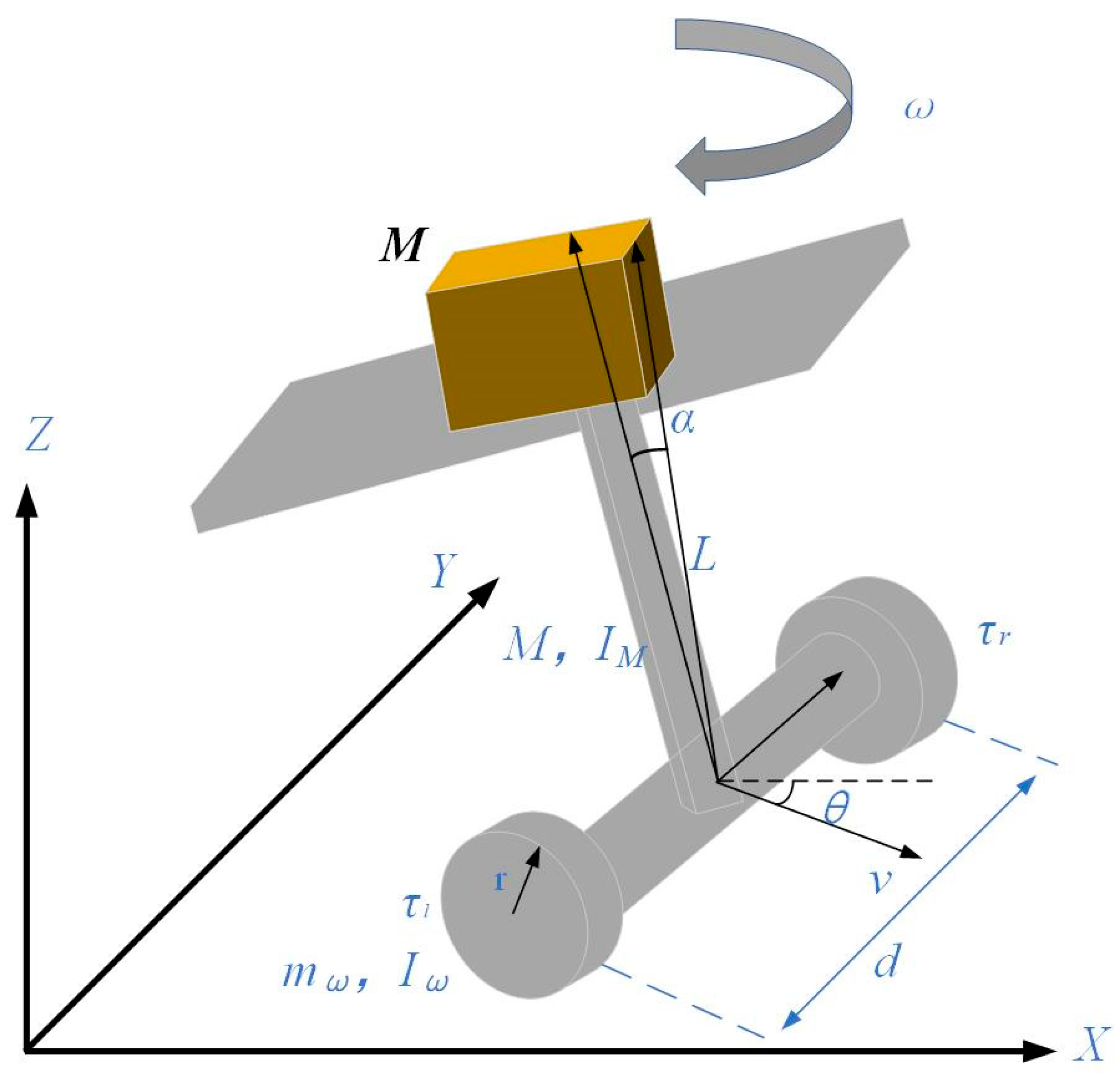
A WIPR is a wheeled inverted pendulum transport robot with a placement table, as illustrated in Figure 1. Its left and right wheels are independent drive wheels that control the robot’s movement speed, rotation direction, and tilt angle of the pendulum using the principle of differential drive to manage the position and posture of WIPR. The generalized world coordinate system is denoted $\mathrm{\Sigma }OXYZ$ while $\left(x,y\right)$, representing the center coordinate of the robot wheels. The robot’s forward velocity and rotational angular velocity are denoted as $v$ and $w$, respectively. The angle of the robot’s direction of motion concerning the $X$-axis is represented by $\theta$, while $\alpha$ is the tilt angle of the pendulum concerning the $Z$-axis. $M$ refers to the total weight of the transport platform plus the pendulum, whereas m denotes the weight of each drive wheel. The distance between the two wheels is represented by $d$, while ${\tau }_r$, and ${\tau }_l$ are the torque of the right wheel and the left wheel, respectively. The rotational inertia of each driven wheel is denoted by $I_w$ and $I_M$ represents the rotational inertia of the transport platform and the pendulum together. The length of the pendulum is represented by $L$. Detailed introduction of robot parameters can be seen in

Table 1. Parameter descriptions.

Parameter	Description
$m_w$	Mass of each wheel
$M$	The total weight of the transport platform plus the pendulum
$I_w$	The rotational inertia of each driven wheel
$I_M$	The rotational inertia of the transport platform and the pendulum
$d$	The distance between the two wheels
$L$	The length of the pendulum
${\tau }_l$	The torque of the left wheel
${\tau }_r$	The torque of the right wheel
$v$	WIPR forward velocity
$w$	WIPR rotation velocity
$\theta$	WIPR Yaw angle
$\alpha$	The tilt angle of the pendulum

.

Remark 1.

The forward velocity of MWIPR is $x_v$, and $x_v=\dot{x}\cos \theta +\dot{y}\sin \theta$.

Assumption 1.

The tires of the MWIPR do not experience any skidding, and there is no potential for lateral deflection during its motion.

According to Assumption 1, the incomplete constraint equation of WIPR in Equation (1) can be listed as follows:

$$\dot{x}\sin \theta -\dot{y}\cos \theta =0,$$

(1)

The position and posture of the WIPR in the world coordinate system are represented by $q={\left[x,y,\theta ,\alpha \right]}^T$. As the Lagrangian modeling method does not require the inclusion of internal forces within the system, it is a quick and straightforward method of building a model. This property makes it particularly well-suited for constructing multivariable and nonlinear dynamic models for the WIPR, as demonstrated in this paper. By dividing $q$ into $q_m$ and $\alpha$, the position of the robot in the coordinate system is denoted by $q_m$, while the angle of the pendulum is represented by $\alpha$. Therefore, the Lagrangian method [31] is employed to establish the dynamic model of the WIPR, and the resulting mathematical model is presented below as Equation (2).

$$\begin{gathered} \left[\begin{array}{cc}{M}_m\left(q\right)& M_{m\alpha }\left(q\right)\\ M_{\alpha m}\left(q\right)& M_{\alpha }\left(q\right)\end{array}\right]\left[\begin{array}{c}{\ddot{q}}_m\\ \ddot{\alpha }\end{array}\right]+\left[\begin{array}{cc}{C}_m\left(q\right)& C_{m\alpha }\left(q\right)\\ C_{\alpha m}\left(q\right)& C_{\alpha }\left(q\right)\end{array}\right]\left[\begin{array}{c}{\dot{q}}_m\\ \dot{\alpha }\end{array}\right]+\left[\begin{array}{c}{G}_m\\ G_{\alpha }\end{array}\right] \\ =\left[\begin{array}{c}{B}_m\left(q_m\right){\tau }_m\\ 0\end{array}\right]+\left[\begin{array}{c}{A}^T\left(q_m\right)\lambda \\ 0\end{array}\right]+\left[\begin{array}{c}{d}_m\\ d_{\alpha }\end{array}\right], \end{gathered}$$

(2)

By defining $A\left(q_m\right)=\left[\sin \theta ,-\cos \theta ,0\right]$, the incompleteness constraint of Equation (1) yields the following result:

$$A\left(q_m\right)q_m=0,$$

(3)

The WIPR system’s incomplete constraint force is $A^T\left(q_m\right)\lambda$, where $\lambda$ is the Lagrange Multiplier. To eliminate the constraint forces in the system, we seek to find a matrix $S\left(q_m\right)\in {ℝ}^{3\times 2}$ that satisfies $S^T\left(q_m\right)A^T\left(q_m\right)=0$.

By defining $\nu ={\left[v,w\right]}^T$, therefore, Equation (4) can be deduced.

$${\dot{q}}_m=S\left(q\right)\nu ,$$

(4)

To eliminate the incompetent constraint forces, a new vector $\dot{\zeta }={\left[{\dot{\zeta }}_1,{\dot{\zeta }}_2,{\dot{\zeta }}_3\right]}^T$$={\left[v,w,\dot{\alpha }\right]}^T$ is defined and used to transform the equation. The transformation involves multiplying both sides of the equation by a scalar $S^T\left(q_m\right)$, resulting in Equation (5):

$$M\left(q\right)\ddot{\zeta }+C\left(q,\dot{q}\right)\dot{\zeta }+G\left(q\right)=\tau +{\tau }_d,$$

(5)

The dynamics of the system can be described using the following equation, in which $M\left(q\right)\in {ℝ}^{3\times 3}$ represents the inertia matrix, $C\left(q,\dot{q}\right)\dot{q}\in {ℝ}^{3\times 3}$ is the Coriolis force matrix, $G\left(q\right)\in {ℝ}^{3\times 1}$ is the gravity matrix, $\tau$ is the control input matrix, and ${\tau }_d$ is the total unknown disturbance. The detailed expressions of each vector or matrix are presented below.

$$\begin{gathered} M\left(q\right)=\left[\begin{array}{cc}{S}^T{M}_{m}S& S^T{M}_m{}_{\alpha }\\ M_{\alpha m}S& M_{\alpha }\end{array}\right]=\left[\begin{array}{ccc}{m}_{11}& 0& m_{13}\\ 0& m_{22}& 0\\ m_{31}& 0& m_{33}\end{array}\right],C\left(q,\dot{q}\right)=\left[\begin{array}{cc}{S}^T{C}_{m}S+S^T{M}_m\dot{S}\hfill & C_{m\alpha }\hfill \\ C_{\alpha m}S+M_{\alpha m}\dot{S}\hfill & C_{\alpha }\hfill \end{array}\right] \\ \left[\begin{array}{ccc}0& 0& c_{13}\\ 0& c_{22}& c_{23}\\ 0& c_{32}& 0\end{array}\right],G\left(q\right)=\left[\begin{array}{c}{S}^T{G}_m\\ G_{\alpha }\end{array}\right]=\left[\begin{array}{c}0\\ 0\\ g_3\end{array}\right]=\left[\begin{array}{c}0\\ 0\\ -MgL\sin \alpha \end{array}\right],\tau =\left[\begin{array}{c}{S}^T{B}_m\left(q_m\right){\tau }_m\\ 0\end{array}\right]=\left[\begin{array}{c}{\tau }_1\\ {\tau }_2\\ 0\end{array}\right] \\ {\tau }_d=\left[\begin{array}{c}{S}^T{d}_m\\ d_{\alpha }\end{array}\right]=\left[\begin{array}{c}{d}_1\\ d_2\\ d_3\end{array}\right]. \end{gathered}$$

The value of each variable in the expression is indicated as $m_{11}=2m+2I_M/r^2+M$, $m_{13}=m_{31}=ML\cos \alpha$, $m_{22}=d^{2}m/2+I_M{d}^2/2r^2+I_{\omega }+M{L}^2{\sin }^2\alpha$, $m_{33}=M{L}^2+I_M$, $c_{22}=\left(1/2\right)M{L}^2\dot{\alpha }{\sin }^2\left(2\alpha \right)$, $c_{23}=-\left(1/2\right)\omega M{L}^2\sin \left(2\alpha \right)$, $c_{13}=-ML\dot{\alpha }\sin \alpha$, $c_{32}=$$-\left(1/2\right)\omega M{L}^2\sin \left(2\alpha \right)$.

Due to the coupling of the state variables in the system, Equation (5) is decoupled into Equation (6).

$$\left\{\begin{array}{l}\left(m_{11}{m}_{33}-m_{13}{m}_{31}\right){\ddot{\zeta }}_1-m_{13}{c}_{32}{\dot{\zeta }}_2+m_{33}{c}_{13}{\dot{\zeta }}_3-m_{13}{g}_3\hfill \\ =m_{33}\left({\tau }_1+d_1\right)-m_{13}{d}_3\hfill \\ m_{22}{\ddot{\zeta }}_2+c_{22}{\dot{\zeta }}_2+c_{23}{\dot{\zeta }}_3={\tau }_2+d_2\hfill \\ \left(m_{11}{m}_{33}-m_{13}{m}_{31}\right){\ddot{\zeta }}_3+m_{11}{c}_{32}{\dot{\zeta }}_2-m_{31}{c}_{13}{\dot{\zeta }}_3+m_{11}{g}_3\hfill \\ =m_{11}{d}_3-m_{31}\left({\tau }_1+d_1\right)\hfill \end{array}\right.,$$

(6)

By defining ${\xi }_1={\left[{\zeta }_1,{\zeta }_2,{\zeta }_3\right]}^T,{\xi }_2={\left[{\dot{\zeta }}_1,{\dot{\zeta }}_2,{\dot{\zeta }}_3\right]}^T$, Equation (6) is converted to Equation (7).

$$\left\{\begin{array}{l}{\dot{\xi }}_1={\xi }_2\hfill \\ {\dot{\xi }}_2=f\left(\xi \right)+g\left(\xi \right)\tau +D\hfill \end{array}\right.,$$

(7)

where

$$\begin{gathered} f\left(\xi \right)=\left[\begin{array}{c}{f}_1\\ f_2\\ f_3\end{array}\right]=\left[\begin{array}{c}\frac{1}{\mathsf{\Omega }}\left(m_{13}{c}_{32}{\dot{\zeta }}_2-m_{33}{c}_{13}{\dot{\zeta }}_3-m_{13}{g}_3\right)\\ \frac{1}{m_{22}}\left(-c_{22}{\dot{\zeta }}_2-c_{23}{\dot{\zeta }}_3\right)\\ \frac{1}{\mathsf{\Omega }}\left(m_{11}{c}_{32}{\dot{\zeta }}_2-m_{31}{c}_{13}{\dot{\zeta }}_3+m_{11}{g}_3\right)\end{array}\right],g\left(\xi \right)=\left[\begin{array}{c}\frac{m_{33}}{\mathsf{\Omega }}\\ \frac{1}{m_{22}}\\ \frac{-m_{31}}{\mathsf{\Omega }}\end{array}\right], \\ D=\left[\begin{array}{c}{D}_1\\ D_2\\ D_3\end{array}\right]=\left[\begin{array}{c}\frac{m_{33}{d}_1-m_{13}{d}_3}{\mathsf{\Omega }}\\ \frac{d_2}{m_{22}}\\ \frac{m_{11}{d}_3-m_{31}{d}_1}{\mathsf{\Omega }}\end{array}\right]. \end{gathered}$$

where $\mathsf{\Omega }=m_{11}{m}_{33}-m_{13}{m}_{31}$.

2.2. The Design of the Kinematic Control Law

In kinematic trajectory tracking control for a WIPR, the system can be simplified to a general two-wheeled non-complete mobile robot for trajectory tracking. The process involves utilizing a reference trajectory state vector $q_m{}_r={\left[x_r,y_r,{\theta }_r\right]}^T$, an actual state vector $q_m={\left[x,y,\theta \right]}^T$, and a control objective designed to manage linear and angular velocities. The objective is to ensure that the actual robot travel trajectory aligns with the reference trajectory, even if the trajectory error $q_{me}={\left[e_x,e_y,e_{\theta }\right]}^T={\left[x_r-x,y_r-y,{\theta }_r-\theta \right]}^T$ approaches zero. To meet the requirement expressed above, the control laws for $v_d$ and $w_d$ can be devised as Equation (8).

$$\underset{t\to \infty }{\lim }\Vert q_{me}\Vert =0,$$

(8)

The Lyapunov function is selected as Equation (9).

$$V_1=\frac{1}{2}{x}_e^2+\frac{1}{2}{y}_e^2+1-\cos {\theta }_e,$$

(9)

While the error persists, the value $V_1$ remains greater than zero, thereby rendering the function positive definite. Equation (10) describes the derivative of $V_1$.

$$\begin{gathered} {\dot{V}}_1=e_x{\dot{e}}_x+e_y{\dot{e}}_y+{\dot{e}}_{\theta }\sin e_{\theta } \\ =e_x\left(w{e}_y-v+v_r\cos e_{\theta }\right)+e_y\left(-w{e}_x+v_r\sin e_{\theta }\right)+\left(w_r-w\right)\sin e_{\theta } \\ =-v{e}_x-w\sin e_{\theta }+e_x{v}_r\cos e_{\theta }+e_y{v}_r\sin e_{\theta }+w_r\sin e_{\theta }\le 0, \end{gathered}$$

(10)

Lyapunov’s stability theorem [32] establishes that the system can achieve asymptotic stability if the function is negative definite, i.e., if ${\dot{V}}_1\le 0$. Accordingly, the sought control law is as follows (11).

$$\left\{\begin{array}{l}{v}_d=v_r\cos e_{\theta }+k_1{e}_x\hfill \\ w_d=w_r+v_r{e}_y+k_2\sin e_{\theta }\hfill \end{array}\right.,$$

(11)

Both $k_1$ and $k_2$ are positive constants.

Substituting the control law into ${\dot{V}}_1$ gives the following equation.

$$\begin{gathered} {\dot{V}}_1=-e_x\left(v_r\cos e_{\theta }+k_1{e}_x\right)-\left(w_r+v_r{e}_y+k_2\sin e_{\theta }\right)\sin e_{\theta }+e_x{v}_r\cos e_{\theta }+e_y{v}_r\sin e_{\theta }+w_r\sin e_{\theta } \\ =-e_x{v}_r\cos e_{\theta }+e_x{v}_r\cos e_{\theta }-k_1{e}_x^2-w_r\sin e_{\theta }+w_r\sin e_{\theta }-v_r{e}_y\sin e_{\theta }+e_y{v}_r\sin e_{\theta }-k_2{\sin }_{e_{\theta }}^2 \\ =-k_1{e}_x^2-k_2{\sin }_{e_{\theta }}^2\le 0. \end{gathered}$$

(12)

Therefore, ${\dot{V}}_1\le 0$ can be proven.

So far, the desired velocity required for the design of the dynamical system is shown in Equation (11), and the velocity tracking problem of the dynamical system and the angle tracking problem of the pendulum will be solved next.

2.3. The Design of NDO

A nonlinear disturbance observer is developed to estimate the actual disturbance in the system for an unknown disturbance D, thereby strengthening the system’s robustness. To address practical considerations, it is assumed that any disturbance is bounded as follows [33,34,35].

Lemma 1.

For initial conditions that are bounded, a Liapunov function is also uniformly bounded $x\left(t\right)$ if there exists a continuous positive definite Liapunov function $V\left(x\right)$ satisfying the following conditions:

$${\delta }_1\left(\Vert x\Vert \right)\le V\left(x\right)\le {\delta }_2\left(\Vert x\Vert \right),\dot{V}\left(x\right)\le -\kappa V\left(x\right)+c,$$

(13)

where ${\delta }_1,{\delta }_2:{ℝ}^n\to ℝ$ is the $V$ class function, and $\kappa ,c$ all are positive constants.

Assumption 2.

Since no disturbance can be infinite in the real world, we assume that the perturbations in the WIPR system studied in this paper are all bounded, and their first-order derivatives and second-order derivatives are assumed to be bounded; thus, the following equations can be obtained.

$$\Vert \dot{D}\Vert \le {\epsilon }_1,\Vert \ddot{D}\Vert \le {\epsilon }_2,{\epsilon }_1>0,{\epsilon }_2>0$$

$\Vert \cdot \Vert$ represents the Euclidean norm of the vector. The NDO is designed as in Equation (14).

$$\begin{gathered} \widehat{D}=Z_1+P_1\left({\xi }_2\right){\dot{Z}}_1=-L_1\left({\xi }_2\right)\left[f\left(\xi \right)+g\left(\xi \right)\tau +\widehat{D}\right]+\widehat{\dot{D}} \\ \widehat{\dot{D}}=Z_2+P_2\left({\xi }_2\right){\dot{Z}}_2=-L_2\left({\xi }_2\right)\left[f\left(\xi \right)+g\left(\xi \right)\tau +\widehat{D}\right], \end{gathered}$$

(14)

$\widehat{D}$ and $\widehat{\dot{D}}$ represent the estimates of the total perturbation and its derivative, respectively, while $Z_1$ and $Z_2$ are intermediate variables in the observer. To meet the requirements of the system, the self-designed nonlinear functions $P_1\left({\xi }_2\right)$ and $P_2\left({\xi }_2\right)$ are used and must satisfy the conditions $L_1\left({\xi }_2\right)=\frac{\partial P_1\left({\xi }_2\right)}{\partial {\xi }_2}$ and $L_2\left({\xi }_2\right)=\frac{\partial P_2\left({\xi }_2\right)}{\partial {\xi }_2}$.

Property 1.

The error between the estimated and actual values of the disturbance is represented by $\tilde{D}=D-\widehat{D}$, while$\tilde{\dot{D}}=\dot{D}-\widehat{\dot{D}}$represents the error between the derivative of the actual value of a perturbation and the derivative of the estimated value of the same perturbation.

The derivation of $\tilde{D}$ and $\tilde{\dot{D}}$ substitution of Equations (7) and (14) into the above equation leads to results $\dot{\tilde{D}}$ and $\tilde{\dot{D}}$, which are the equations of the NDO, (15) and (16), respectively.

$$\begin{gathered} \dot{\tilde{D}}=\dot{D}-\dot{\widehat{D}}=\dot{D}-{\dot{Z}}_1-\frac{\partial P\left({\xi }_2\right)}{\partial {\xi }_2}\cdot \frac{d{\xi }_2}{dt}=\dot{D}-{\dot{Z}}_1-L_1\left({\xi }_2\right){\dot{\xi }}_2 \\ =\dot{D}+L_1\left({\xi }_2\right)\left[f\left(\xi \right)+g\left(\xi \right)\tau +\widehat{D}\right]-\widehat{\dot{D}}-L_1\left({\xi }_2\right){\dot{\xi }}_2 \\ \dot{D}+L_1\left({\xi }_2\right)\left[f\left(\xi \right)+g\left(\xi \right)\tau +\widehat{D}\right]-\widehat{\dot{D}}-L_1\left({\xi }_2\right)\left[f\left(\xi \right)+g\left(\xi \right)\tau +D\right] \\ =-L_1\left({\xi }_2\right)\tilde{D}+\tilde{\dot{D}}, \end{gathered}$$

(15)

$$\begin{gathered} \dot{\tilde{\dot{D}}}=\ddot{D}-\dot{\widehat{\dot{D}}}=\dot{D}-{\dot{Z}}_2-\frac{\partial P\left({\xi }_2\right)}{\partial {\xi }_2}\cdot \frac{d{\xi }_2}{dt}=\ddot{D}-{\dot{Z}}_2-L_2\left({\xi }_2\right){\dot{\xi }}_2 \\ =\ddot{D}+L_2\left({\xi }_2\right)\left[f\left(\xi \right)+g\left(\xi \right)\tau +\widehat{D}\right]-L_2\left({\xi }_2\right)\left[f\left(\xi \right)+g\left(\xi \right)\tau +D\right] \\ =-L_2\left({\xi }_2\right)\tilde{D}+\ddot{D}, \end{gathered}$$

(16)

By letting $E={\left[{\tilde{D}}^T,{\tilde{\dot{D}}}^T\right]}^T$ and substituting the appropriate Equations (15)–(17) can be obtained.

$$\dot{E}=LE+\delta \ddot{D},$$

(17)

where $L=\left[\begin{array}{cc}-L_1\left({\xi }_2\right)& I_3\\ -L_2\left({\xi }_2\right)& 0\end{array}\right]$, $\delta =\left[\begin{array}{c}0\\ I_3\end{array}\right]$. The observer’s stability is examined, and a Lyapunov function is selected to make sure that it can reliably predict the system state despite any nonlinear disturbances. By selecting an appropriate Liapunov function, we rigorously prove the stability of the observer and the precision of its estimation precisely.

Property 2.

$L$ is a skew-symmetric matrix.

$$V_2=\frac{1}{2}{E}^{T}E,$$

(18)

The proof of the derivative of $V_2$ can be expressed as follows:

$${\dot{V}}_2=E^T\dot{E}=E^T\left(LE+\delta \ddot{D}\right)\le E^T\left(L+0.5\Vert \delta {\Vert }^2{I}_6\right)E+0.5{\epsilon }_2^2,$$

(19)

The above design of an NDO for a WIPR can be summarized in the following theorem.

Theorem 1.

For the existence of an unknown disturbance in a WIPR system, the perturbation estimation error is bounded for the observer designed according to Equation (14).

Proof. 

The design parameters $L_1\left({\xi }_2\right)=\frac{\partial P_1\left({\xi }_2\right)}{\partial {\xi }_2}$ and $L_2\left({\xi }_2\right)=\frac{\partial P_2\left({\xi }_2\right)}{\partial {\xi }_2}$ are such that $L+0.5\Vert \delta {\Vert }^2{I}_6$ is a negative definite matrix, according to Lemma 1, then $E$ is bounded. □

2.4. The Design of Improved Slide Mode Control

The sliding mode control algorithm consists of two key elements: (i) the design of the sliding mode surface; and (ii) the design of the convergence rate. The design of the sliding mode surface is mainly based on the system structure as well as the control objective. As for the design of convergence law, there are four different convergence laws: the isokinetic convergence law, exponential convergence law, power convergence law, and general convergence law. In this paper, based on the optimal control objective of WIPPR to cope with nonlinearity and underdrive, as well as unknown disturbances, the traditional exponential convergence law is improved by introducing an adaptive control function, and an improved sliding mode control based on the adaptive exponential convergence law is proposed, which can weaken the system jitter while speeding up the system response, making the sliding mode control more suitable for tracking the reference trajectory of the WIPR system under the action of unknown disturbances [36]. The design for the traditional exponential convergence law is shown in Equation (20).

$$\dot{s}=-\eta \mathrm{sgn}\left(s\right)-\mu s,$$

(20)

where: $s$ denotes the slip surface function; the parameters $\eta$, $\mu$ denote the convergence coefficient; and $\mathrm{sgn}\left(s\right)$ denotes the sign function.

In the traditional exponential convergence law, the isokinetic term is denoted $-\eta \mathrm{sgn}\left(s\right)$, and the exponential term is denoted $-\mu s$. When the state of the system is far from the slip surface, the exponential term and the isokinetic term in the convergence law act simultaneously to help the system move toward the slip surface, and the magnitude of the isokinetic term and the exponential term are mainly determined by the reference $\eta$, $\mu$. The exponential term is small, and the isokinetic term acts mainly when the system is moving close to the surface.

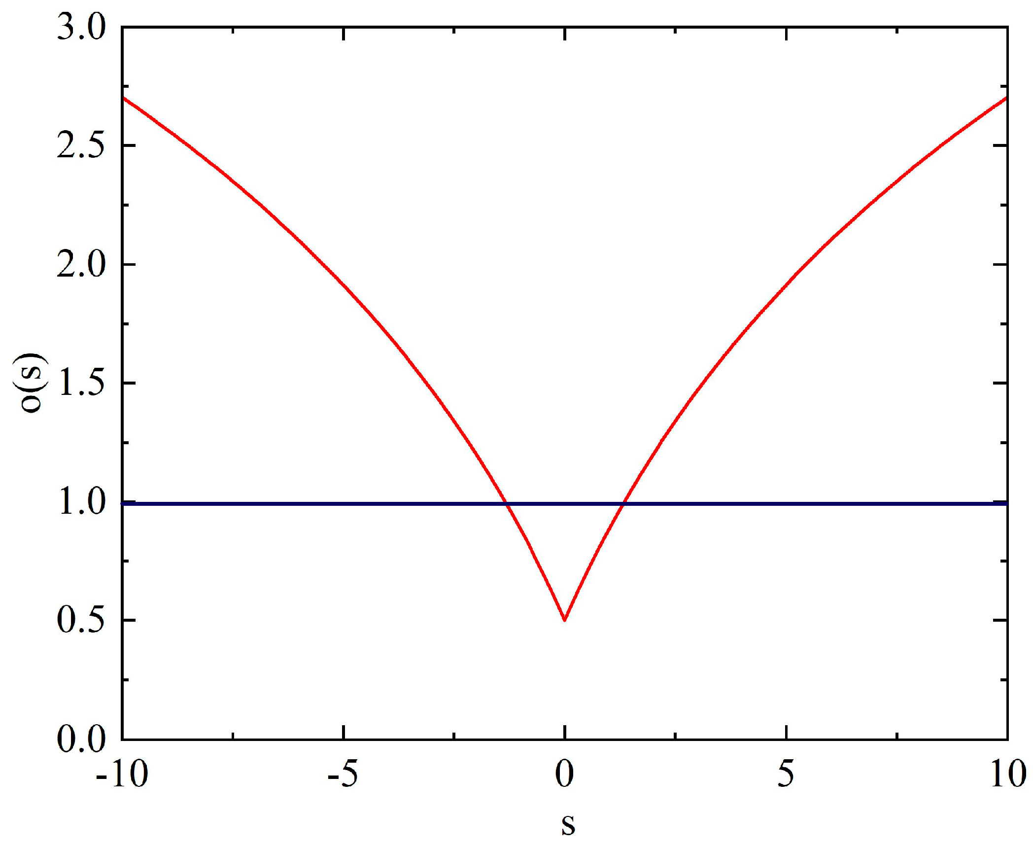
This paper makes a corresponding improvement based on the traditional exponential convergence law and introduces the adaptive $o\left(s\right)$ function to adjust the convergence law in accordance with the control state of the system, as shown in Figure 2, which can accelerate the convergence speed of the sliding mode and weaken the overshoot phenomenon. This allows the sliding mode control to reduce the jitter phenomenon of the system. Following the inclusion of the adaptive function $o\left(s\right)$, the new exponential convergence law is as follows:

$$\left\{\begin{array}{l}\dot{s}=-\eta o\left(s\right)\mathrm{sgn}\left(s\right)-\mu s\hfill \\ o\left(s\right)=\frac{\left(\left|s\right|+1\right)\left[{\log }_a\left(\left|s\right|+a\right)\right]}{\left|s\right|+{\log }_a\left(\left|s\right|+a\right)+b}\hfill \end{array}\right.,$$

(21)

where $a>0$, $b>0$, $\eta >0$, $\mu >0$.

Through the analysis, relative to not adding the adaptive function (i.e., o(s) = 1), it can be found that when the system motion point is far away from the sliding surface (namely, when s is far away from the origin 0), the adaptive function $o\left(s\right)$ will increase the convergence law, which will speed up the system convergence speed, shorten the system state convergence time to the target state, and reduce the control time; when the system motion point is close to the sliding surface, $\left|s\right|$ will converge to 0 and $o\left(s\right)$ will be less than 1. The role of $o\left(s\right)$ here is to suppress the jitter amplitude and weaken the state variable fluctuation problem after the system is stabilized, and the suppression effect will be more obvious as the parameter $b$ increases. To further weaken the jitter problem of the stabilized system, the smoothing process is carried out for the symbolic function $\mathrm{sgn}\left(s\right)$ in this paper, which is known as the traditional symbolic function [37], as shown in the following equation.

$$\mathrm{sgn}\left(s\right)=\left\{\begin{array}{l}1s>0\hfill \\ 0s=0\hfill \\ -1s<0\hfill \end{array}\right.,$$

(22)

The symbolic function after the smoothing process is shown below.

$$\mathrm{sgn}\left(s\right)=\frac{s}{\left|s\right|+\beta },\beta =0.01,$$

(23)

2.5. The Design of the Forward-Rotation Subsystem

For convenience, the system has been reorganized into the following form (24).

$$\left\{\begin{array}{l}{\ddot{\zeta }}_1=\frac{1}{\mathsf{\Omega }}\left(m_{13}{c}_{32}{\dot{\zeta }}_2-m_{33}{c}_{13}{\dot{\zeta }}_3-m_{13}{g}_3\right)+\frac{m_{33}}{\mathsf{\Omega }}{\tau }_1+D_1\hfill \\ {\ddot{\zeta }}_2=\frac{1}{m_{22}}\left(-c_{22}{\dot{\zeta }}_2-c_{23}{\dot{\zeta }}_3\right)+\frac{1}{m_{22}}{\tau }_2+D_2\hfill \end{array}\right.,$$

(24)

The state variables in the system described by Equation (24) are highly coupled. To address this issue and to expand the system’s asymptotic stability domain, a hierarchical sliding mode controller was designed. The controller’s primary objective is to utilize an input control law that can simultaneously control both system variables ${\zeta }_1$ and ${\zeta }_2$, thereby, mitigating the problem of system coupling [38].

Having obtained the expected forward velocity ($v_d$) and angular velocity ($w_d$) from Equation (11), the error between the actual and expected values can be defined as follows:

$$\left\{\begin{array}{l}{e}_{x_v}={\zeta }_{1d}-{\zeta }_1=x_r\cos {\theta }_r+y_r\sin {\theta }_r-x_v\hfill \\ e_v={\dot{\zeta }}_{1d}-{\dot{\zeta }}_1=v_d-v\hfill \\ e_{\theta }={\zeta }_{2d}-{\zeta }_2={\theta }_r-\theta \hfill \\ e_w={\dot{\zeta }}_{2d}-{\dot{\zeta }}_2=w_d-w\hfill \end{array}\right.,$$

(25)

To design the sliding mode control error tracking scheme for the $v$-$w$ subsystem, two mutually independent first-layer sliding mode surfaces were initially constructed. The equations used to create these slide surfaces are as follows:

$$s_1={\gamma }_1{e}_{x_v}+e_v,{\gamma }_1>0,$$

(26)

$$s_2={\gamma }_2{e}_{\theta }+e_w,{\gamma }_2>0,$$

(27)

The results of deriving Equations (26) and (27) are presented below.

$$\begin{gathered} {\dot{s}}_1={\gamma }_1{\dot{e}}_{x_v}+{\dot{e}}_v={\gamma }_1{\dot{e}}_{x_v}+{\ddot{\zeta }}_{1d}-{\ddot{\zeta }}_1=0 \\ {\dot{s}}_2={\gamma }_2{\dot{e}}_{\theta }+{\dot{e}}_w={\gamma }_2{\dot{e}}_{\theta }+{\ddot{\zeta }}_{2d}-{\ddot{\zeta }}_2=0, \end{gathered}$$

(28)

According to Filippov’s equivalent control theory, the equivalent control laws for ${\zeta }_1$ and ${\zeta }_2$ are as follows:

$$\left\{\begin{array}{l}{\tau }_{eq1}=-\frac{\Delta }{m_{33}}\left({\gamma }_1{\dot{e}}_{x_v}+{\ddot{\zeta }}_{1d}+{\widehat{D}}_1\right)+\frac{1}{m_{33}}\left(m_{13}{c}_{32}{\dot{\zeta }}_2-m_{33}{c}_{13}{\dot{\zeta }}_3-m_{13}{g}_3\right)\hfill \\ {\tau }_{eq2}=m_{22}\left({\gamma }_2{\dot{e}}_{\theta }+{\ddot{\zeta }}_{2d}\right)+c_{22}{\dot{\zeta }}_2+c_{23}{\dot{\zeta }}_3-{\widehat{D}}_2\hfill \end{array}\right.$$

(29)

The second sliding surface can be expressed as a linear combination of the first sliding surface.

$$s_3={\gamma }_3{s}_1+{\gamma }_4{s}_2,{\gamma }_{3,}{\gamma }_4>0,$$

(30)

To control ${\zeta }_1$ and ${\zeta }_2$, the equivalent control law must be included at the same time to control and enter their designed sliding surface, respectively. Therefore, the total control law is shown in the following equation.

$${\tau }_u={\tau }_{eq1}+{\tau }_{eq2}+{\tau }_{sw},$$

(31)

${\tau }_{sw}$ is the switching law of the converging slide surface phase, and the expressions are as follows.

$${\tau }_{sw}=\frac{-\left({\gamma }_3\frac{m_{22}}{\mathsf{\Omega }}{\tau }_{eq2}+{\gamma }_4\frac{1}{m_{22}}{\tau }_{eq1}+{\eta }_{1}o\left(s_3\right)\mathrm{sgn}\left(s_3\right)+{\mu }_1{s}_3\right)}{{\gamma }_3\frac{m_{22}}{\mathsf{\Omega }}+{\gamma }_4\frac{1}{m_{22}}},$$

(32)

To mitigate the jitter phenomenon of the system, the isokinetic and exponential terms of the sliding mode control are improved, where ${\eta }_1$ and ${\mu }_1$ are the isokinetic and exponential terms of the previous design convergence law, and both are positive constants; $o\left(s_3\right)$ and $\mathrm{sgn}\left(s_3\right)$ are the adaptive and symbolic functions designed in the previous paper. To prove that the designed controller is stable, the Lyapunov function is chosen as follows.

$$V_3=\frac{1}{2}{s}_3^2>0$$

(33)

The derivative of $V_3$ for time is given by the following expression.

$$\begin{gathered} {\dot{V}}_3=s_3{\dot{s}}_3=s_3\left({\gamma }_3{\dot{s}}_1+{\gamma }_4{\dot{s}}_2\right)=s_3\left[{\gamma }_3\left({\gamma }_1{\dot{e}}_{x_v}+{\dot{e}}_v\right)+{\gamma }_4\left({\gamma }_2{\dot{e}}_{\theta }+{\dot{e}}_w\right)\right]=s_3\left[{\gamma }_3\left({\gamma }_1{\dot{e}}_{x_v}+{\dot{v}}_d-\dot{v}\right)+{\gamma }_4\left({\gamma }_2{\dot{e}}_{\theta }+{\dot{w}}_d-\dot{w}\right)\right] \\ =s_3\left\{{\gamma }_3\left[{\gamma }_1{\dot{e}}_{x_v}+{\dot{v}}_d-f_1-\frac{m_{33}}{\mathsf{\Omega }}\left({\tau }_{eq1}+{\tau }_{eq2}+{\tau }_{sw}\right)-D_1\right]\right.+\left.{\gamma }_3\left[{\gamma }_2{\dot{e}}_{\theta }+{\dot{w}}_d-f_2-\frac{1}{m_{22}}\left({\tau }_{eq1}+{\tau }_{eq2}+{\tau }_{sw}\right)-D_2\right]\right\} \\ =s_3\left[-{\eta }_{1}o\left(s_3\right)\mathrm{sgn}\left(s_3\right)-{\mu }_1{s}_3^2+{\gamma }_1\left({\widehat{D}}_1-D_1\right)+{\gamma }_2\left({\widehat{D}}_2-D_2\right)\right]\le -{\eta }_{1}o\left(s_3\right)\left|s_3\right|-{\mu }_1{s}_3^2+\left|s_3\right|\left({\gamma }_1\left|{\tilde{D}}_1\right|+{\gamma }_2\left|{\tilde{D}}_2\right|\right) \end{gathered}$$

(34)

By design ${\eta }_{1}o\left(s_3\right)>{\gamma }_1\left|{\tilde{D}}_1\right|+{\gamma }_2\left|{\tilde{D}}_2\right|$, the result of the following equation can be obtained.

$${\dot{V}}_3\le -{\eta }_1{s}_3^2\le -\frac{{\eta }_1}{2}{V}_3$$

(35)

From Lemma 1 in [38], the following equation can be obtained.

$$V_3\left(t\right)\le e^{-\frac{{\eta }_1}{2}\left(t-t_0\right)}V\left(t_0\right)$$

(36)

It can be seen that the $V_3\left(t\right)$ index converges to 0, and the rate of convergence depends on ${\eta }_1$.

As demonstrated by the preceding equation, the error state can attain the slip surface in a finite amount of time. Subsequently, the first layer of slip surfaces $s_1$ and $s_2$ can converge asymptotically to zero, leading to the convergence of both the rotational and forward velocities of WIPR to the desired values.

2.6. The Design of the Tilt-Angle Subsystem

The system discussed in the previous section can achieve complete tracking of ${\zeta }_1$ and ${\zeta }_2$ within a finite time, which enables us to transform it into the following form:

$${\ddot{\zeta }}_3=\frac{1}{\mathsf{\Omega }}\left(m_{11}{c}_{32}{\dot{\zeta }}_{2d}-m_{31}{c}_{13}{\dot{\zeta }}_3+m_{11}{g}_3\right)-\frac{m_{31}}{\mathsf{\Omega }}{\tau }_3+D_3,$$

(37)

As WIPR aims to maintain a vertical and stable direction of the pendulum during its motion, all relevant parameters (${\alpha }_d,{\dot{\alpha }}_d,{\ddot{\alpha }}_d$) can be set to zero. As such, the following definitions can be employed:

$$\left\{\begin{array}{l}{e}_{\alpha }={\alpha }_d-\alpha =-\alpha \hfill \\ e_{\dot{\alpha }}={\dot{\alpha }}_d-\dot{\alpha }=-\dot{\alpha }\hfill \end{array}\right.,$$

(38)

Let the sliding mode surface be defined as Equation (39), with its derivative expressed as Equation (40).

$$s_4={\gamma }_5{e}_{\alpha }+e_{\dot{\alpha }},$$

(39)

$${\dot{s}}_4={\gamma }_5{\dot{e}}_{\alpha }+{\dot{e}}_{\dot{\alpha }}=-{\gamma }_5\dot{\alpha }-\ddot{\alpha }=-{\eta }_{2}o\left(s_4\right)\mathrm{sgn}\left(s_4\right)-{\mu }_2{s}_4,$$

(40)

After substituting Equation (37), the control law for the tilt angle subsystem can be derived as presented in Equation (41).

$${\tau }_{\alpha }=-\frac{\mathsf{\Phi }}{m_{31}}\left({\gamma }_5\dot{\alpha }+{\widehat{D}}_3\right)-\frac{1}{m_{31}}(m_{11}{c}_{12}{\dot{\zeta }}_2-m_{31}{c}_{13}{\dot{\zeta }}_3+m_{11}{g}_3-{\eta }_{2}o\left(s_4\right)\mathrm{sgn}\left(s_4\right))-{\mu }_2{s}_4$$

(41)

To prove the stability of the designed system, the Lyapunov function is chosen as follows.

$$V_4=\frac{1}{2}{s}_4^2$$

(42)

The derivative of $V_4$ for time is given by the following expression.

$$\begin{gathered} {\dot{V}}_4=s_4{\dot{s}}_4=s_4\left(-{\gamma }_5\dot{\alpha }-\ddot{\alpha }\right)=s_4\left(-{\gamma }_5\dot{\alpha }-f_3-\frac{1}{m_{22}}{\tau }_{\alpha }-D_3\right) \\ =s_4\left[-{\eta }_{2}o\left(s_4\right)\mathrm{sgn}\left(s_4\right)-{\mu }_2{s}_4^2+{\gamma }_5\left({\widehat{D}}_3-D_3\right)\right]\le -{\eta }_{2}o\left(s_4\right)\left|s_4\right|-{\mu }_2{s}_4^2+{\gamma }_5\left|{\tilde{D}}_3\right| \end{gathered}$$

(43)

By choosing ${\eta }_{2}o\left(s_4\right)>{\gamma }_5\left|{\tilde{D}}_3\right|$, it enables ${\dot{V}}_4<0$ to hold, indicating that the system achieves asymptotic stability.

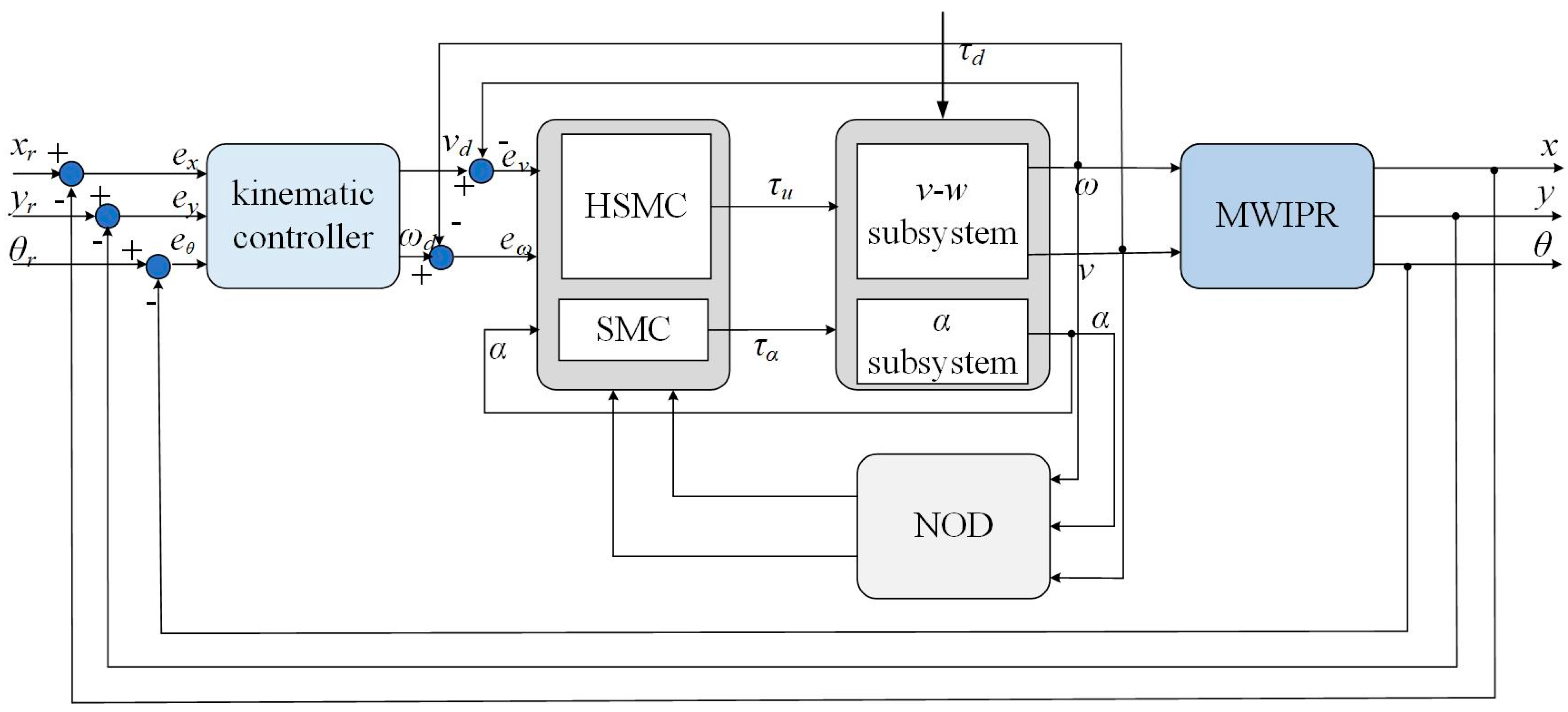
Figure 3 displays the schematic block diagram of the control system.

3. Simulation

The focus of this section is to discuss the trajectory-tracking effect of the system in a simulation environment, and to verify the feasibility of the proposed control scheme and what the advantages of the proposed method are compared with other control systems in this paper. Next, the simulation results of different control systems in the face of the same disturbance will be compared to verify the control effectiveness of each system. The parameters in the system are shown in the following

Table 2. The value of each parameter variable in the system.

Parameter (Unit)	Value
$M\left(\mathrm{kg}\right)$	8
$m\left(\mathrm{kg}\right)$	0.5
$I_M\left(\mathrm{kg}\cdot {\mathrm{m}}^2\right)$	5
$I_w\left(\mathrm{kg}\cdot {\mathrm{m}}^2\right)$	0.3
$d\left(\mathrm{m}\right)$	0.5
$L\left(\mathrm{m}\right)$	0.5
$r\left(\mathrm{m}\right)$	0.1

.

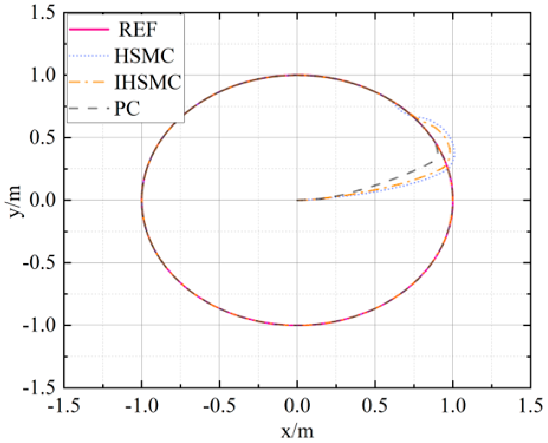
The simulation experiments in Matlab/Simulink verified the high-precision trajectory tracking capability of the system and the stability of the pendulum in robot motion. During the simulation study, the initial position was set as $q_m={\left[0,0,0\right]}^T$, and the initial position of the reference trajectory was set as $q_m{}_r={\left[0,0,\pi /2\right]}^T$, where the desired tracking velocity = 1 m/s and the angular velocity = 1 rad/s. Therefore, the trajectory of the robot should be a circle with a radius of 1 m, and the center of the circle is $\left(0,0\right)$. Therefore, the time function of the reference trajectory was chosen as $\left\{x=\sin t,y=\cos t\right\}$.

An external perturbation was added, as shown in the following equation.

$$\left\{\begin{array}{l}{D}_1=0.4\sin \left(0.4t\right)Nm\hfill \\ D_2=0.5\cos \left(0.5t\right)Nm\hfill \\ D_3=0.6\sin \left(0.6t\right)Nm\hfill \end{array}\right.,$$

(44)

To demonstrate the superiority of the proposed method in this paper, three comparative experiments were conducted under the given disturbance conditions: the first experiment involved the simulation results of the unimproved HSMC method, the second experiment involved the simulation results of the improved IHSMC method with adaptive law but without nonlinear disturbance observer, and the third experiment involved the simulation results of the proposed method in this paper (referred to as PC).

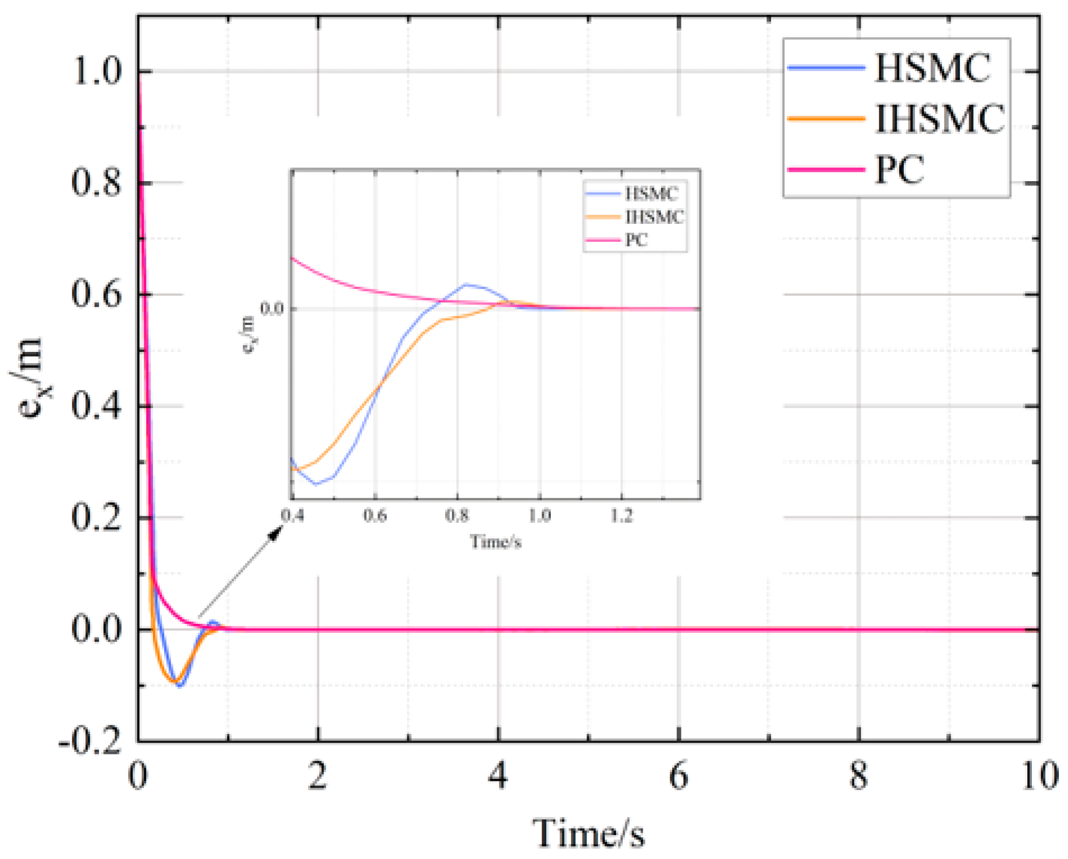
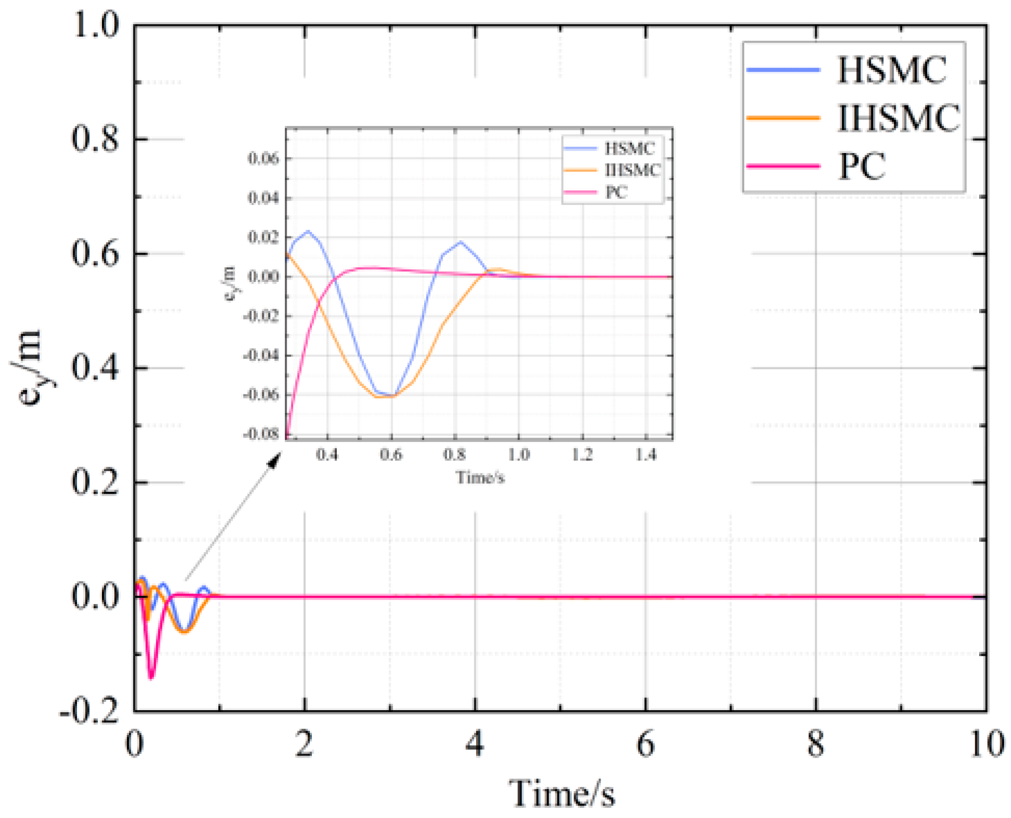
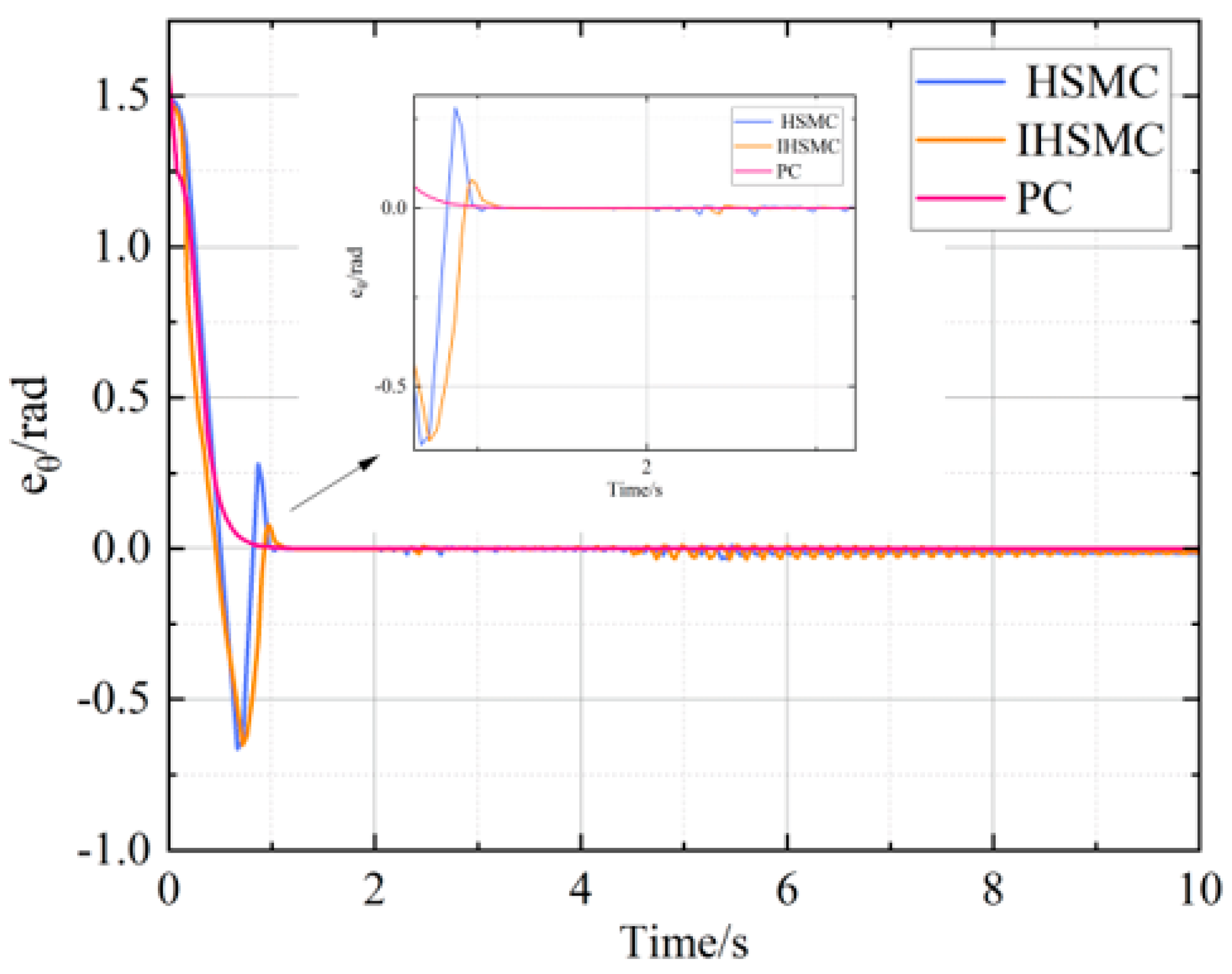
First of all, by observing Figure 4, Figure 5 and Figure 6, it can be concluded that the proposed method in this paper is better than the other two control methods in terms of both the speed of convergence of the error to the steady state and the magnitude of the fluctuation of the error after reaching the steady state when compared with the other two methods. This undoubtedly reflects the effectiveness of the method in this paper, which can track the given reference trajectory very accurately.

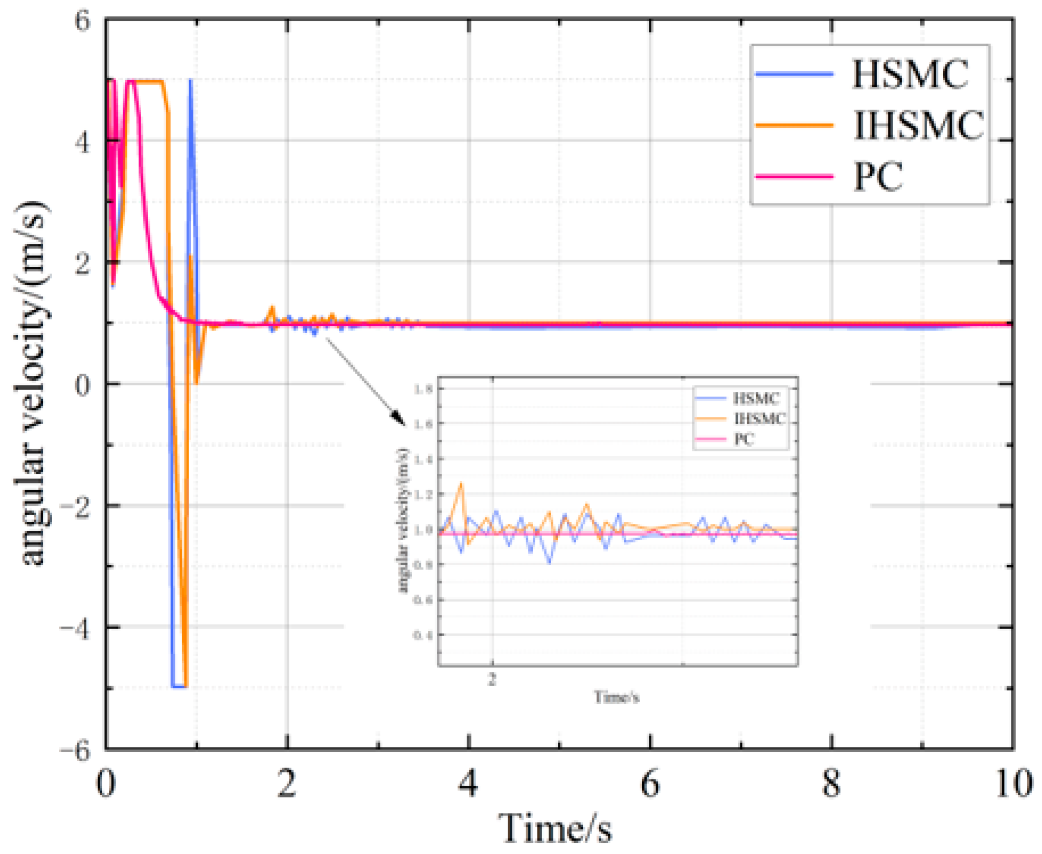
Figure 7 and Figure 8 give the tracking of the desired speed of the WIPR system under the three control methods. Compared with the other two methods, firstly, the control method in this paper can track the desired speed more rapidly, reaching the effect of tracking the desired speed at 0.7 s, whereas the other two methods track the desired speed in more than 1 s, which is much slower than the method in this paper, and the fluctuation frequency is high, which may affect the stability of the WIPR. As can be seen from Figure 8, the present method exceeds the other two methods in the tracking effect of rotational velocity relative to the forward velocity, for one. The convergence speed is fast, and more importantly, the proposed method is very stable after the velocity tracking reaches the steady state, which can be regarded as showing no fluctuation compared with the other two methods.

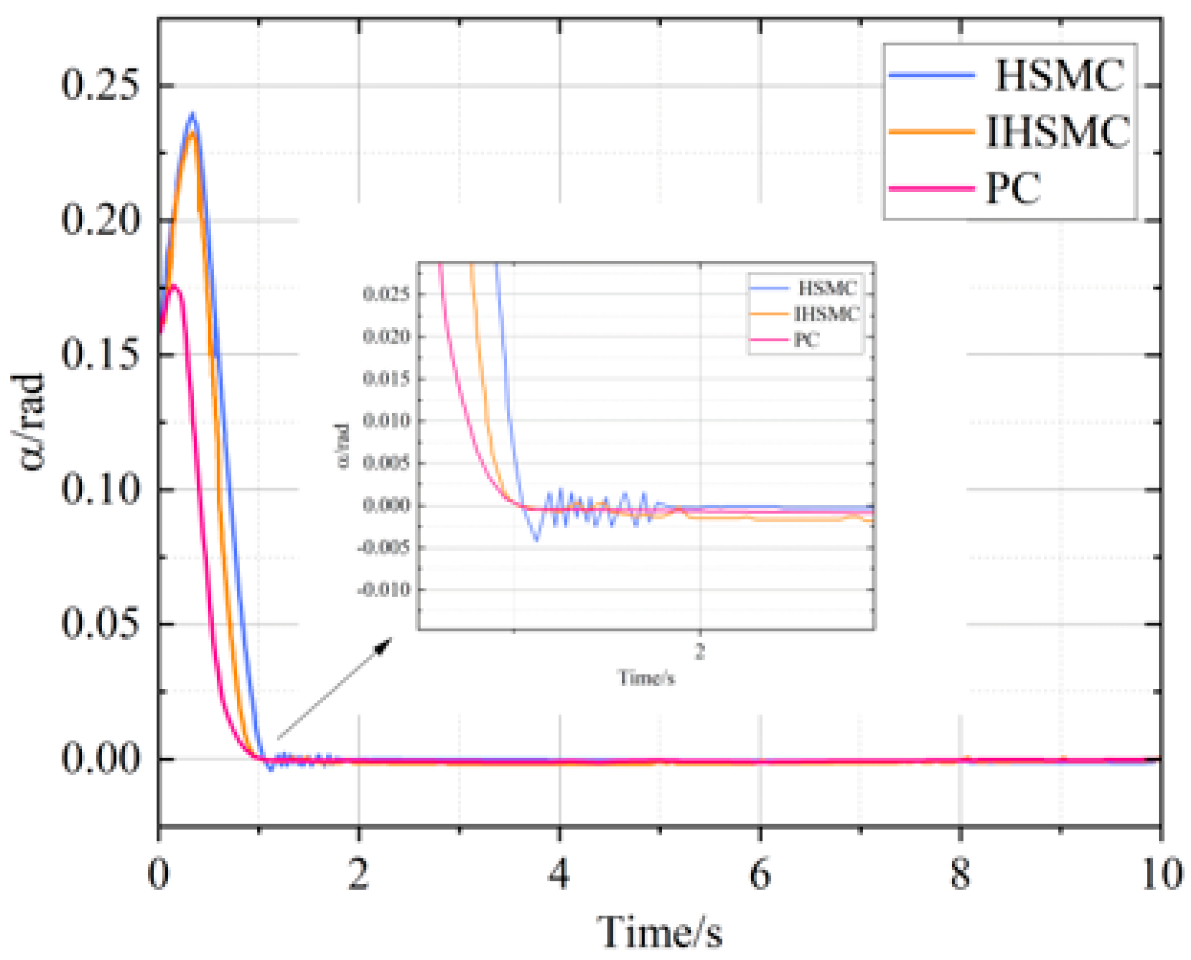
The HSMC method with general exponential convergence law has more frequent angle oscillations, and the system is more unstable, as can be seen from the angle change of the WIPR pendulum shown in Figure 9, whereas the IHSMC improved convergence law method’s pendulum has smoother oscillations after reaching stability, and the control effect is obviously stronger than that of the HSMC with general exponential convergence law. In terms of response time and maximum overshoot, the suggested method outperforms the other two ways, and it can continue to operate smoothly and without oscillations once it has reached the stabilization point.

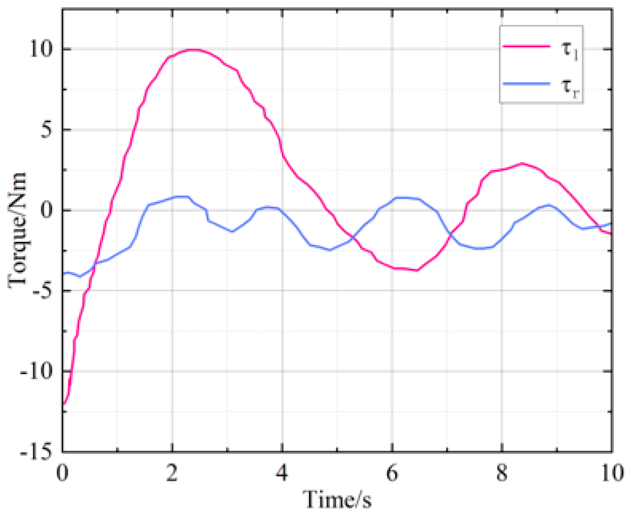
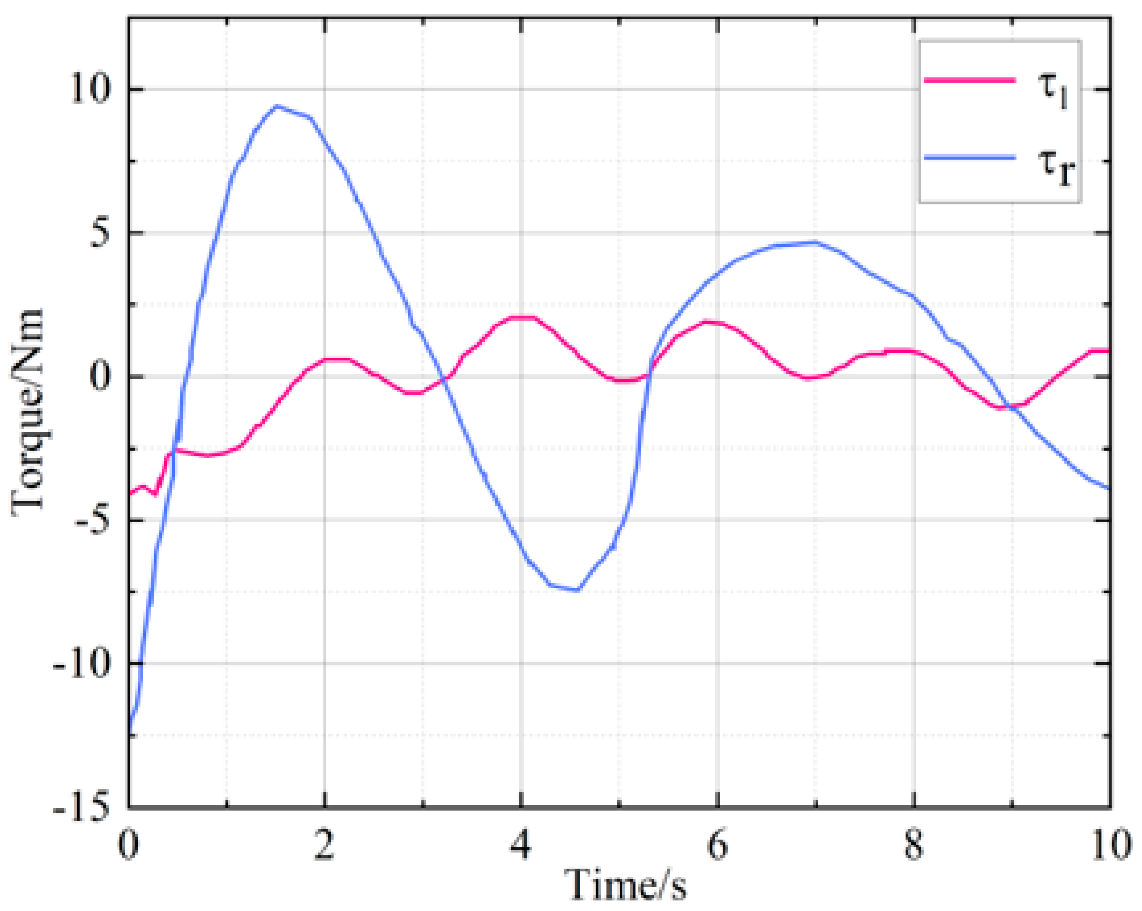
The variograms of the input torque for the three control methods are presented in Figure 10, Figure 11 and Figure 12. The results indicate that when the convergence law of HSMC follows the general exponential convergence law, the jitter vibration of the input torque for the left and right wheels of WIPR is evident, which adversely affects the output of the actuator (i.e., affects the output of the drive motors of the left and right wheels). In contrast, Figure 11 illustrates that the improved convergence law significantly reduces the jitter phenomenon, resulting in a more beneficial improvement for the actuator.

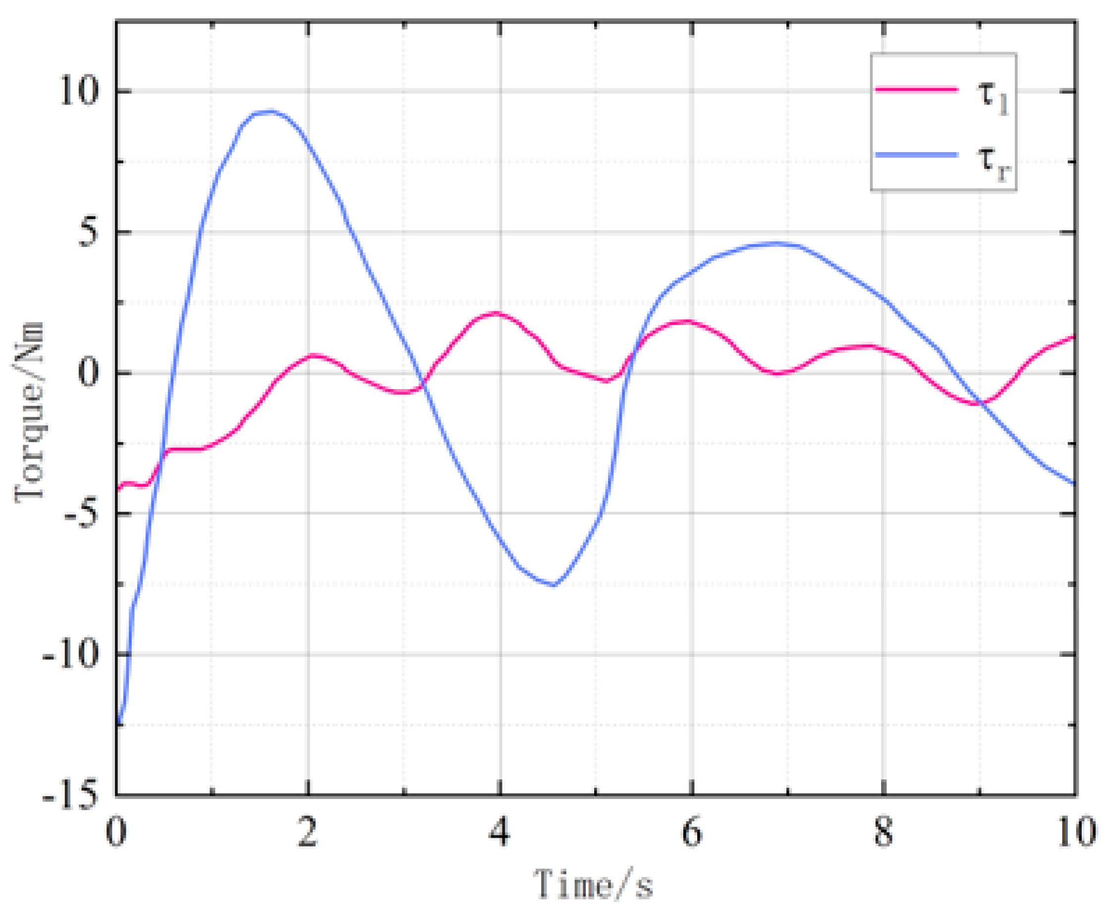
Figure 12 presents the variation of input torque under the proposed control method. It can be observed that the input torque obtained by this method is smoother than IHSMC, and the jitter suppression effect is more satisfactory. This approach achieves a better torque input graph, making it the most effective method among the three for actuator benefits. Therefore, the proposed control method demonstrates superior performance in terms of reducing jitter and enhancing actuator benefits compared with the other two control methods, making it a better solution.

Figure 13 shows the trajectory tracking diagrams of different control systems. From an intuitive point of view, the proposed scheme is also significantly better than the other two schemes. As shown by the simulation comparison experiment, the method proposed in this paper is feasible, and its effect is excellent.

4. Conclusions

The purpose of this paper was to study the trajectory-tracking problem for WIPRs and propose a hierarchical sliding mode controller with a nonlinear perturbation observer to achieve accurate control of the reference trajectory and maintain the pendulum stability during motion. A nonlinear disturbance observer was designed to make the system more robust to unknown external disturbances. The underdriven coupling of WIPRs was addressed by dividing the system into two subsystems through the decoupling of its control state variables. The hierarchical sliding mode control method with an improved convergence law was then applied to control the system and suppress the “jitter” phenomenon. Finally, the Lyapunov function was chosen to verify the stability of the system mathematically.

The feasibility of the control system was verified using simulation software. However, considering the complexity of the real-world environment and external uncertainty, future work will focus on building a hardware system for the robot to study the real effects of the control method of WIPRs in the real world.