Article

Preoperative Prediction of Optimal Femoral Implant Size by Regularized Regression on 3D Femoral Bone Shape

by
Adriaan Lambrechts
1,*,
Christophe Van Dijck
1,
Roel Wirix-Speetjens
1,
Jos Vander Sloten
2,
Frederik Maes
3,4 and
Sabine Van Huffel
5
1
Materialise NV, 3001 Leuven, Belgium
2
Biomechanics Section, Mechanical Engineering, KU Leuven, 3001 Leuven, Belgium
3
Processing Speech and Images (PSI), Department of Electrical Engineering (ESAT), KU Leuven, 3001 Leuven, Belgium
4
Medical Imaging Research Center, UZ Leuven, 3000 Leuven, Belgium
5
STADIUS Center for Dynamical Systems, Signal Processing and Data Analytics, Department of Electrical Engineering (ESAT), KU Leuven, 3001 Leuven, Belgium
*
Author to whom correspondence should be addressed.
Appl. Sci. 2023, 13(7), 4344; https://doi.org/10.3390/app13074344
Submission received: 28 February 2023 / Revised: 20 March 2023 / Accepted: 23 March 2023 / Published: 29 March 2023
(This article belongs to the Special Issue Novel Advances in Computer-Assisted Surgery)

Abstract

:
Preoperative determination of implant size for total knee arthroplasty surgery has numerous clinical and logistical benefits. Currently, surgeons use X-ray-based templating to estimate implant size, but this method has low accuracy. Our study aims to improve accuracy by developing a machine learning approach that predicts the required implant size based on a 3D femoral bone mesh, the key factor in determining the correct implant size. A linear regression framework imposing group sparsity on the 3D bone mesh vertex coordinates was proposed based on a dataset of 446 MRI scans. The group sparse regression method was further regularized based on the connectivity of the bone mesh to enforce neighbouring vertices to have similar importance to the model. Our hypergraph regularized group lasso had an accuracy of 70.1% in predicting femoral implant size while the initial implant size prediction provided by the instrumentation manufacturer to the surgeon has an accuracy of 23.1%. Furthermore, our method was capable of predicting the implant size up to one size smaller or larger with an accuracy of 99.1%, thereby surpassing other state-of-the-art methods. The hypergraph regularized group lasso was able to obtain a significantly higher accuracy compared to the implant size prediction provided by the instrumentation manufacturer.

1. Introduction

Knee osteoarthritis is a degenerative disease affecting the knee cartilage layers. Due to progressive knee cartilage wear, patients can experience pain, instability, loss of flexibility, joint stiffness and swelling. For patients with severe knee osteoarthritis, a total knee arthroplasty (TKA) surgery can help improve quality of life [1]. During a TKA procedure the femur and tibial bones are resected along the joint interface and replaced by metal components. Two-dimensional templating is the most frequently used method to preoperatively determine the required implant size. In 2D templating, anteroposterior and lateral radiographs are overlaid with 2D template shapes of the implants to determine the best fitting size. Despite its broad adoption, 2D templating has relatively low accuracy in determining the required size due to the nature of projection images [2,3,4,5]. Three-dimensional templating based on computed tomography (CT) or magnetic resonance imaging (MRI) scans can overcome this limitation of 2D templating resulting in higher templating accuracy [6,7,8]. Three-dimensional templating allows the surgeon to position the implants on a 3D model of the joint to determine the optimal implant size and position.
There are several benefits to preoperatively planning the implant size. First of all, determining the correct implant sizes is of importance from a clinical point of view. Femoral oversizing might lead to irritation of the soft-tissue structures surrounding the joint, increased patellofemoral pressure or reduced range of motion and, hence, should be avoided [9]. On the other hand, femoral undersizing can lead to femoral fracture due to anterior implant notching, flexion instability, or inferior patellar tracking due to a medialized implant placement [10]. Secondly, the extremely large and small implant sizes need to be specifically ordered as they are not consistently present in the hospital [11]. Furthermore, knowing the implant size up to a size smaller or larger reduces the sterilization cost and operation room setup time [12,13].
Over recent decades, machine learning has been successfully applied to many medical applications, including implant size templating [14,15,16]. Several studies have investigated implant size prediction based on demographic data [2,11,16,17,18,19,20,21,22]. The method by Trainor et al. used only shoe size and gender to obtain the highest reported accuracy of 63% and an accuracy of 99% for predicting up to one size larger or smaller [11]. Finally, Lambrechts et al. created a support vector machine based model that predicts implant size based on manually defined features deduced from 3D bone models, resulting in an absolute accuracy of 82.2%, significantly higher compared to models relying on demographic data [23].
Traditional methods for determining implant size are based on human predefined measurements. However, surgeons base the implant size on the size and morphology of the bone. Therefore, we hypothesize that shape based implant size prediction can yield higher accuracy compared to previously investigated methods. To the best of our knowledge, our method is the first to regress the implant size directly based on the 3D model of the bone. The computational method most similar to the one presented in this study, is an optimal-scoring-based method by Clemmensen et al. that induces sparsity [24]. This algorithm was evaluated on a classification task distinguishing male and female face silhouettes based on the point coordinates. The method by Clemmensen et al. obtains interpretability by introducing sparsity through the use of l 1 regularization on the model coefficients corresponding to single coordinates of certain points. As a result, this method can only find directions of shape variations that are parallel to the coordinate system axes which is a major disadvantage. A second limitation is that proximity information is not incorporated into the model as neighbouring points in space should have similar contribution to the model.
Therefore, we propose a method that extends the method by Clemmensen et al. in multiple ways. Firstly, our method is targeted toward triangular meshes allowing better incorporation of spatial structure compared to point clouds. Secondly, group lasso regularization was used to obtain directions of variation in bone shape which are predictive of our target. As opposed to the method by Clemmensen et al., our method allows these directions of variation to be in any direction, not only parallel to coordinate axes. Thirdly, connectivity of the mesh structure is included in our model as extra prior information.

2. Materials and Methods

2.1. Data Preprocessing

For our model we used a dataset of 446 TKA preoperative plans retrospectively collected. All cases were planned by a single surgeon based on an MRI scan of the patient’s knee joint. MRI scans have as benefit the visualization of the knee bone, as well as cartilage which can aid the surgeon during 3D templating. The MRI scan protocol is described in Table 1. The scans were semi-automatically segmented (Mimics, Materialise, Belgium) by experienced conversion engineers. The segmented mask contains both the bone and the cartilage of femur. Next, these masks were converted to a triangulated surface mesh based on the marching cubes algorithm [25]. For each patient the corresponding femoral implant size planned by the surgeon was also available. All patients received a posterior-stabilized Zimmer-Biomet Vanguard implant, which has 10 possible sizes.
Our group lasso method relies on meshes which have point correspondences and identical adjacency matrices. To achieve this, we employ a previously developed statistical shape model (SSM) which was created based on a training set of 524 MRI scans independent from the dataset used for training the hypergraph regularized group lasso [26]. The SSM was fitted to all bones in the dataset to obtain point correspondence. Next, a non-rigid surface registration is applied to register the fitted model to the target femur [27]. Finally the vertex coordinates of the registered femur meshes are stacked in a matrix X R N × 3 p , where N indicates the number of femur meshes in the dataset, and p the number of points in the mesh. Finally, all columns of the data matrix X are scaled to have a mean of zero and a standard deviation of 1. The implant sizes are coded as an ordinal variable with a range from 1 to 10, represented by y . Based on a stratified split, 70% of the samples are used for creating the model and the remaining samples form the test set to measure the final accuracy of the model.

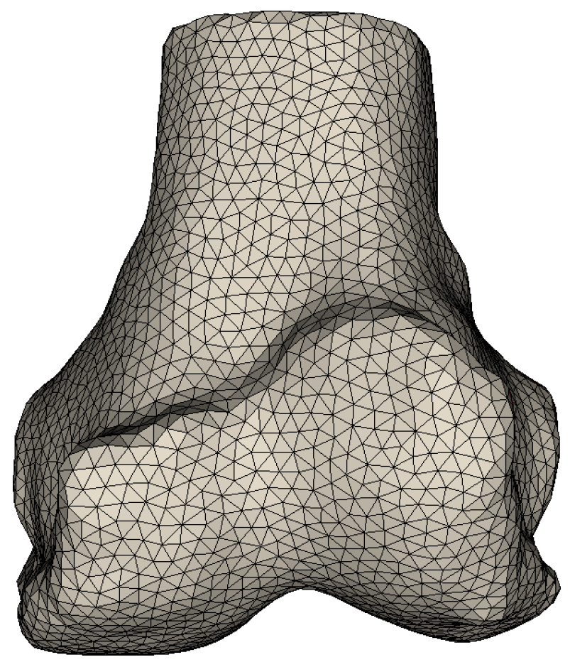
2.2. Hypergraph Representation of a Triangular Mesh

A triangular mesh can be represented as a simple undirected graph characterized by a set of vertices and edges: G = ( V , E ) . Figure 1 represents a femur mesh with edges represented as black lines. Simple graphs can be represented by a Laplacian matrix L R p × p , defined as the difference of the adjacency and degree matrices. The Laplacian matrix has useful properties for analysing the structure of a graph. However, the simple graph structure of a mesh is not compatible with the regression framework proposed in this study. Therefore, the mesh will be represented by a hypergraph, a generalization of a graph. Hypergraphs have hyperedges which can connect any number of vertices. In a simple graph, each vertex represents a point in 3D space, while for the hypergraph we split each of these points into three vertices: one for each coordinate (Figure 2). All edges of the original graph become hyperedges in the hypergraph connecting 6 vertices, hence it is a 6-uniform hypergraph.
For hypergraphs, the incidence matrix H R | V | × | E | identifies which vertices are part of a hyperedge:
H i j = 1 i f v i E j 0 i f v i E j
Similarly, two diagonal degree matrices can be defined: the edge degree matrix D e R | E | × | E | and the vertex degree matrix D v R | V | × | V | .
D e i j = k = 1 | V | H k i if i = j 0 otherwise D v i j = k = 1 | E | H i k if i = j 0 otherwise
Based on these matrices, the hypergraph Laplacian can be defined as:
L H = D v H D e 1 H T

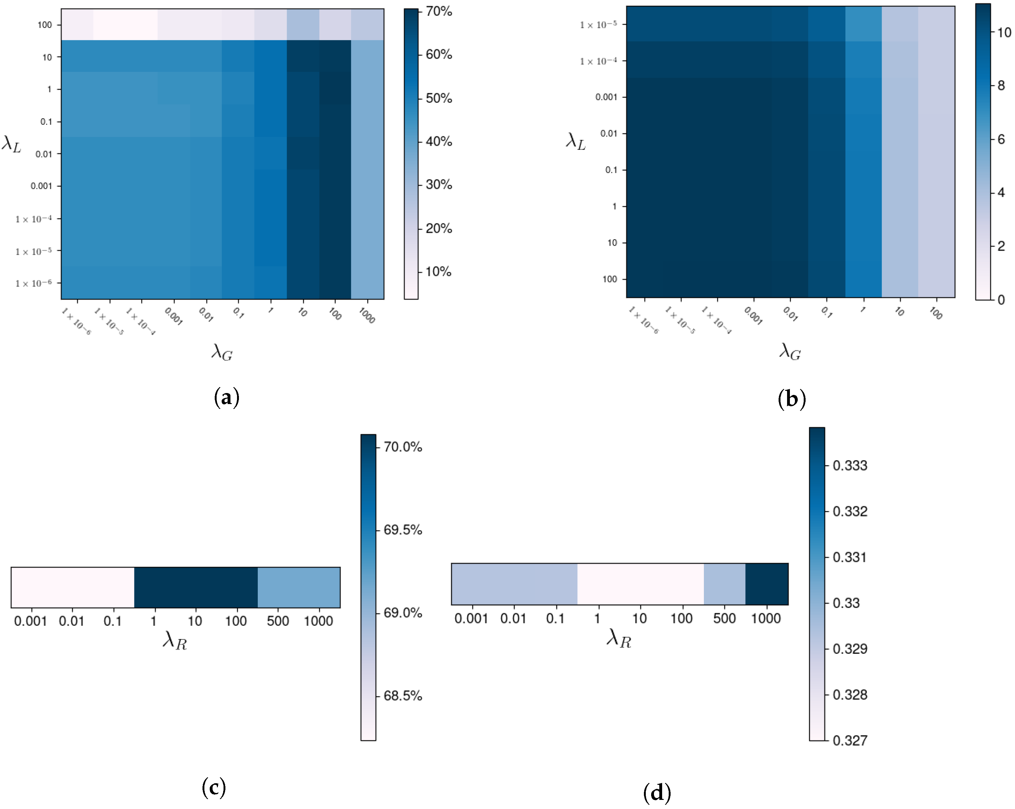
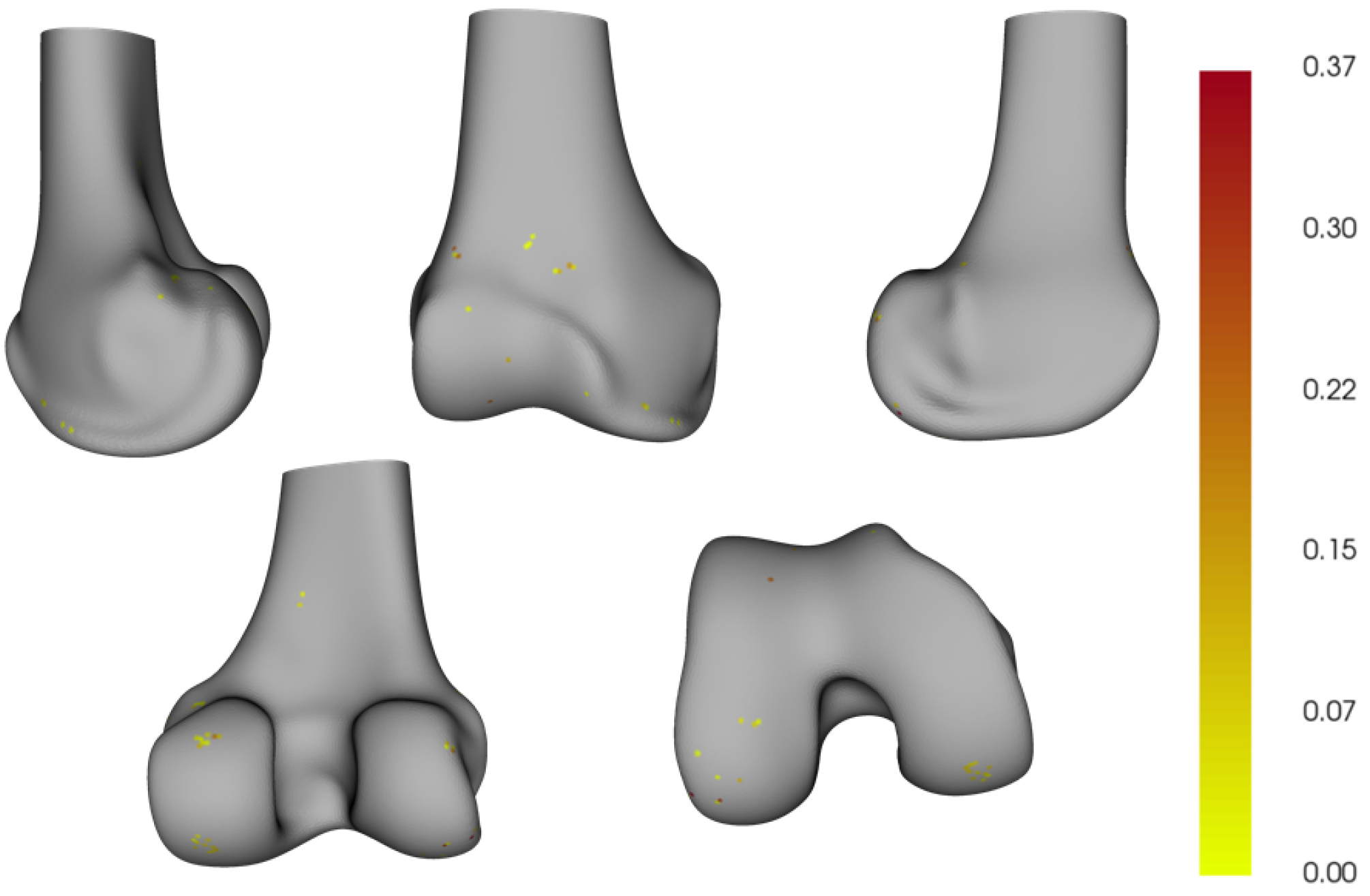
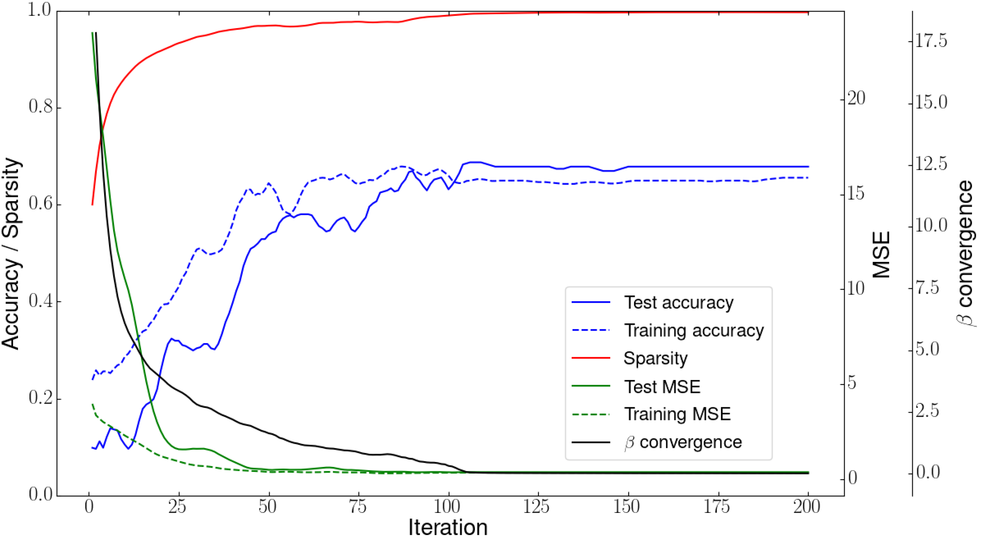
2.3. Hypergraph Regularized Group Lasso

The target of the hypergraph regularized group lasso is to obtain a subset of points on the femur mesh, the coordinates of which can be linearly combined to predict the femur implant size. This can be accomplished by the following optimization problem:
min β 1 2 y X β 2 2 + λ G g P β g 2 + λ L 2 β T L H β + λ R 2 β T I β
The objective function has four terms. The first term is a least squares term trying to represent the implant size y as a linear combination of the vertex locations of the mesh, parameterized by β . The parameter vector β indicates the importance of each vertex’s coordinates in predicting the femoral implant size. The second term is a group lasso regularization term which results in sparsity in the points selected. P is the set of 3-tuples in which each tuple g references the column indices corresponding to the group of { x , y , z } coordinates of a point on the mesh. β g R 3 is a set of 3 of the model parameters corresponding with the { x , y , z } coordinates from point p g . This regularization forces either all coordinates of a point to be included in the model or all coordinates of the point are found to be uninformative to the model, in which case they receive a zero-valued β g coefficient. As a result, the group sparsity term creates model interpretability by expressing the femoral size as a linear combination of a small subset of points on the mesh. The third term forces the model coefficients of vertices linked by an edge, to be similar in value. We opted to use this penalty term because our hypothesis is that vertices linked by an edge are nearby in space, hence they should have a similar influence on the model. The last term is a ridge penalty to obtain uniqueness of the solution. The group lasso itself does not necessarily result in a unique solution because it is not strictly convex [28]. The addition of the ridge regularization leads to a strictly convex function guaranteeing a unique solution.
The group lasso problem is a convex non-differentiable problem as it is discontinuous at β g = 0 . For these types of problems computationally efficient solvers exist based on the proximal gradient method which alternatively optimize each group [29]. Therefore, the objective function should be group separable. However, the hypergraph regularization term is not. Nevertheless, the objective function can be rewritten as a normal group lasso problem which can be solved using the proximal gradient method.
By combining the ridge penalty with the hyper-graph Laplacian regularization, the objective function can be simplified. More specifically, the weighted sum of the identity matrix and the hypergraph Laplacian is a positive definite matrix. Hence, it can be decomposed using a Cholesky decomposition [30]: λ R λ L I + L H = U T U . Using the upper triangular matrix U we augment the feature matrix X and target vector y as follows [31]:
X ˜ = X λ L U R ( N + 3 p ) × 3 p
y ˜ = y 0 3 p R N + 3 p
0 3 p is a column vector with 3 p zero values. Using this augmented data matrix and target vector, the optimization problem can be reformulated as a standard group lasso, which, in turn, is fully group-separable:
min β 1 2 y ˜ g P X ˜ g β g 2 2 + λ G g P β g 2
Tibshirani et al. proposed a proximal gradient solving method to find the optimal solution for this convex problem [29]. The algorithm cycles over each group g and iteratively solves three equations until convergence. This inner iterative loop can be accelerated with the Nesterov acceleration method [32]:
r : = y ˜ i g X ˜ i β i 0 ω g t + 1 = β g t + ν X ˜ g T ( r g X ˜ g β g t ) β g t + 1 = 1 ν λ G ω g t 2 + ω g t + 1 β g t + 1 : = β g t + 1 + t t + 3 ( β g t + 1 β g t )
The ν parameter is the step size in the optimization and should be carefully set to converge sufficiently fast while avoiding divergence from the optimum. ( q ) + : = m a x { 0 , q } is the positive part function. In Equation (8), the superscripts indicate the iteration count. The complete algorithm is described in Algorithm 1. Mathematical operations, such as additions, norm calculation, and matrix-vector products were performed using compressed sparse column operations to reduce both computational time and memory footprint [33]. The algorithm’s accuracy is determined by three parameters λ G , λ R , and λ L , which control the relative strength of the three regularization terms. Larger values of λ G improve the interpretability by reducing the number of points in the final solution. Larger values of λ L improve smoothness of the coefficient values across neighbouring points on the mesh. Finally, larger values of λ R , generally avoid overfitting of the model by reducing the values of the model parameters. To determine the optimal values for these three parameters, a 3D logarithmic grid search approach was combined with five-fold cross validation on the training set. The range of λ G , λ R and λ L started at 10 6 and was increased by a factor of 10 until the value of 1000 was reached.
Algorithm 1: Hypergraph regularized group Lasso.
Applsci 13 04344 i001

2.4. Baseline Method

To establish a baseline, our method was compared against statistical shape mode coefficient-based linear regression. While fitting the SSM to each of the femurs in the dataset, the shape mode coefficients are obtained. These coefficients quantify the presence of the uncorrelated modes of shape variation. For example, the first shape mode variation is generally a measure for bone volume and, hence, should correlate with the required implant size. Using an elastic net, the shape mode coefficients were regressed to the femoral implant size [31]. The hyperparameters of the elastic net were tuned using grid search during a five-fold cross validation procedure.

3. Results

All meshes in the dataset had 22,476 vertices after SSM fitting and non-linear registration resulting in a data matrix X R 312 × 67,428 . The data matrix is augmented with the upper triangular matrix from the Cholesky decomposition resulting in a data matrix of size X ˜ R 67.740 × 67.428 with 88% sparsity. Owing to the sparsity of the problem, it becomes feasible to solve the hypergraph regularized group lasso efficiently through the use of sparse matrix and vector calculations.
The algorithm performance in terms of average accuracy of femoral implant size prediction y ^ and average mean squared error (MSE) over all folds, during the cross-validation procedure, is displayed in Figure 3. Figure 3a,b visualize the effect of λ G and λ L on the accuracy and MSE, respectively, with constant λ R = 1 . Figure 3c,d visualize the effect of λ R on the accuracy and MSE, respectively, for constant λ G = 100 and λ L = 10 . During the cross validation stage the average calculation time for training with one combination of hyperparameters was 28.7 min on an Intel® Xeon® E5-1620 v3 CPU and 64 GB RAM memory.
λ G = 100 , λ L = 10 , and λ R = 1 resulted in optimal performance during cross-validation with a test set accuracy and accuracy up to one size smaller or larger of 70.08% and 99.11%, respectively. The final solution has a sparsity of 99.8%, which represent 43 vertices from the bone mesh with non-zero model coefficients (Figure 4). Gray zones identify vertices with zero coefficients resulting from the model’s sparsity. The vertices have a colour on the scale from yellow to red indicating low to high importance. Figure 5 provides an overview of the model’s performance per iteration of training. The convergence towards the final model coefficients β is defined as β t β t 1 2 2 . One can observe the clear link between sparsity of the solution and the model’s performance in terms of MSE and accuracy. On the other hand, the baseline method obtained a severely lower test set accuracy of 58.9%.
From the model coefficients β , the importance of each point p can be derived by the norm of its corresponding coordinates’ model coefficients: β p 2 . Figure 4 visualizes the vertices importance values of the final model coefficients on different views of the femur. The coefficient vector β g can also be interpreted by the direction it points to, representing the direction of variation which is most sensitive to variation in the implant size changes. In Figure 6, the directions of the model coefficients have been displayed by arrows drawn from vertex location with non-zero β g 2 in the direction of β g . All arrows were normalized to unit length.

4. Discussion

The group sparsity regularization has the largest impact on the model accuracy as shown in Figure 3. For λ L > 10 model performance starts to decrease significantly due to the diminishing effect of sparsity resulting in decreasing generalization. Nevertheless, the effect of the hypergraph regularization cannot be neglected, as can be seen in Figure 3, where the MSE starts to decrease for values of λ L > 0.1 . The L 2 regularization results in the desirable property of uniqueness of the solution. However, at higher values of λ R the accuracy and MSE start to decrease as a result of reduced sparsity.
During the optimizer’s iterations the amount of sparsity increases while the model’s MSE decreases, resulting in model interpretability (Figure 5). The final solution has small clusters of points above the patellofemoral articular cartilage, on the femoral posterior condyles, on the femoral distal condylar area, and around the medial and lateral rim of the femoral distal cartilage layer are selected by the model. These regions also hold important anatomical information for determining femoral implant size. For example, the points selected on the anterior femoral shaft above the patellofemoral articular surface determine whether femoral implant notching might occur due to undersizing, where the implant undercuts the femoral cortical bone surface. Femoral notching is associated with an increased likelihood of supracondular fracture [34]. Therefore, these regions are likely taken into account by the model.
One interesting observation is that vertices in the model are very often present in small clusters of neighbours. This is most likely due to the hypergraph regularization which has a smoothing effect, trying to force neighbouring vertices to have similar model coefficients. These clusters seem to increase the model’s generalization. Our hypothesis is that they make the algorithm more robust against errors in the non-linear registration performed after the SSM fit.
In Figure 6, the directions of bone shape variation which are predictive of the femoral implant size are visualized. All of these directions point outward from the bone indicating, that larger bones result in larger implant sizes, as expected. At first glance, these arrows seem to point normal to the surface of the bone mesh. However, at closer inspection, some β g directions deviate up to 67.8° from the direction of the surface normal. For example, the vertices selected by the model on the distal lateral condyle point significantly more posterior in comparison with the direction of the surface normal at these points. This indicates that the anteroposterior variation in bone shape at the femoral condyles causes a change in femoral implant size, which is conform with clinical knowledge.
Practical implementation of our method could be through a software application which starts from the patient’s MRI scan, and subsequently automatically segments it using previously investigated methods [35]. Next, the application could propose implant size based on the prediction from our proposed model. Alternatively, the model can be integrated in 3D templating software from an implant manufacturer. Our method is compatible with current generation implants with fixed increments between sizes.
Several studies have investigated the accuracy of 2D templating (Table 2) [3,4,5,6,7]. In the table, bold values indicate the best performance per metric. Although 2D templating is frequently performed, it has relatively low accuracy (48–64%). Furthermore, 2D templating is a manual procedure. On the other hand, manual 3D templating shows far greater accuracy of 93.9–100% [4,7,8]. Implant size selection based on manual 3D templating with MRI scans has been shown to have excellent intra- and interclass correlation coefficients amongst surgeons [36]. The intra-class correlation ranged from 96.6% to 99%, and the inter-class correction was 97%. Hence, it is a suitable medium for preoperative assessment of the required implant size. To the best of our knowledge there is only one study which investigated an automatic 2D templating method with 19.2% accuracy [37].
For our dataset, we can compare the accuracy of the model with that of the femoral implant size proposed by the instrumentation manufacturer. The test set accuracy of the femoral implant size proposed by the manufacturer is 23.1%, while our model obtained an accuracy of 70.08%. This accuracy improvement will result in a more efficient planning experience for the surgeon by reducing planning time. However, both the manufacturer’s default and our method obtain the same test set accuracy up to one size larger or smaller of 99.11%. Furthermore, our proposed method also significantly surpasses the baseline method in terms of accuracy.
Our method outperforms other methods relying on demographic data in terms of both the absolute accuracy and the accuracy up to 1 size smaller or larger (Table 3). Therefore, we conclude that geometric features extracted from the 3D anatomical model provide additional information that improves implant size prediction accuracy. Furthermore, all other investigated methods rely on features defined based on clinical expertise. In comparison, our method automatically extracts the relevant features which determine the femoral implant size. The study by Lambrechts et al., (2022) obtained a higher absolute accuracy compared to our currently proposed method, however, it relied on a significant amount of clinical knowledge to extract relevant features from the 3D bone models and uses non-linear models [23]. One of the limitations of this comparison is the difference in focus: our method predicts the preoperatively planned implant size, which differs slightly from the intra-operatively used implant size predicted by the other studies relying on demographic data.
More accurate implant size prediction using our method might positively impact total knee arthroplasty surgery through improved logistics requiring reduced inventory, less trays to sterilize and reduced operating room setup times. These measures might reduce the cost associated with the treatment. Furthermore, accurate templating helps the surgeon to be better prepared for surgery and can potentially reduce the operative times. Nevertheless, these claims need to be further validated.
The advantages of our model are its fast calculation time and the ability to produce accurate results when limited data are available. However, there are also points of improvement. The proposed method was validated for a single surgeon. Hence, further research can be conducted to investigate generalization to a larger population of surgeons. Additional research could look into combining the proposed mesh-based features with relevant demographic data to improve model accuracy. Another limitation is the linearity implied by our model. Possibly, non-linearities could provide higher accuracy through interaction of the vertex coordinates, such as distances or angles. Finally, it could be investigated if this method yields equal improvement for predicting tibial implant sizes. Tibial and femoral implant sizes are correlated and, thus, a method combining both bones could help increase the accuracy.

5. Conclusions

We presented a femoral implant sizing algorithm based on a regression framework mapping the bone mesh vertices locations to the implant size. For this under-determined problem, group sparsity ensured selection of the most predictive vertices on the mesh. Extra prior information was added, through hypergraph regularization, to the optimization problem by including the mesh’s graph structure to constrain neighbouring to have similar impact on the regressed implant size. From our experiments we found that the group sparsity had the largest impact on the model performance, while the hypergraph-based regularization mainly improved robustness. In total, 43 anatomical locations were identified which could be used to predict the implant size. Our method was successful at predicting the femoral implant size, as preoperatively planned by a surgeon. Our method was accurate in 70.08% of test set cases, in determining the femoral implant size in comparison with an accuracy of 23.1% for the implant size provided in the preoperative plan from the instrumentation manufacturer. Towards future work, an extension of the method could include simultaneous prediction of the femoral and tibial implant sizes, since they are correlated. Furthermore, a non-linear model might, such as graph convolutional networks, might improve model performance.

Author Contributions

Conceptualization, A.L., C.V.D., R.W.-S., J.V.S., F.M. and S.V.H.; formal analysis A.L. and C.V.D.; methodology, A.L.; software, A.L. and C.V.D.; validation, A.L.; data curation, A.L.; writing—original draft preparation, A.L.; writing—review and editing, A.L., C.V.D., R.W.-S., J.V.S., F.M. and S.V.H.; supervision, R.W.-S., J.V.S., S.V.H. and F.M. All authors have read and agreed to the published version of the manuscript.

Funding

This research received no external funding.

Data Availability Statement

The data that support the findings of this study consist of restricted data which are not publicly available.

Acknowledgments

Sabine Van Huffel and Frederik Maes received funding from the Flemish Government (AI Research Program)and are both affiliated to Leuven. AI-KU Leuven institute for AI, B-3000, Leuven, Belgium.

Conflicts of Interest

Adriaan Lambrechts, Christophe Van Dijck and Roel Wirix-Speetjens are paid employees of Materialise NV. Jos Vander Sloten is member of the board of directors of Materialise NV.

References

  1. Bourne, R.B.; Chesworth, B.M.; Davis, A.M.; Mahomed, N.N.; Charron, K.D.J. Patient Satisfaction after Total Knee Arthroplasty: Who is Satisfied and Who is Not? Clin. Orthop. Relat. Res. 2010, 468, 57–63. [Google Scholar] [CrossRef] [PubMed] [Green Version]
  2. Wallace, S.J.; Murphy, M.P.; Schiffman, C.J.; Hopkinson, W.J.; Brown, N.M. Demographic data is more predictive of component size than digital radiographic templating in total knee arthroplasty. Knee Surg. Relat. Res. 2020, 32, 63. [Google Scholar] [CrossRef] [PubMed]
  3. Trickett, R.W.; Hodgson, P.; Forster, M.C.; Robertson, A. The reliability and accuracy of digital templating in total knee replacement. J. Bone Jt. Surg. Br. Vol. 2009, 91, 903–906. [Google Scholar] [CrossRef] [PubMed]
  4. Miller, A.G.; Purtill, J.J. Accuracy of digital templating in total knee arthroplasty. Am. J. Orthop. 2012, 41, 510–512. [Google Scholar] [PubMed]
  5. Unnanuntana, A.; Arunakul, M.; Unnanuntana, A. The accuracy of preoperative templating in total knee arthroplasty. J. Med. Assoc. Thail. Chotmaihet Thangphaet 2007, 90, 2338–2343. [Google Scholar]
  6. Pietrzak, J.R.T.; Rowan, F.E.; Kayani, B.; Donaldson, M.J.; Huq, S.S.; Haddad, F.S. Preoperative CT-Based Three-Dimensional Templating in Robot-Assisted Total Knee Arthroplasty More Accurately Predicts Implant Sizes than Two-Dimensional Templating. J. Knee Surg. 2019, 32, 642–648. [Google Scholar] [CrossRef]
  7. Ettinger, M.; Claassen, L.; Paes, P.; Calliess, T. 2D versus 3D templating in total knee arthroplasty. Knee 2016, 23, 149–151. [Google Scholar] [CrossRef]
  8. Schotanus, M.G.M.; Schoenmakers, D.A.L.; Sollie, R.; Kort, N.P. Patient-specific instruments for total knee arthroplasty can accurately predict the component size as used peroperative. Knee Surg. Sport. Traumatol. Arthrosc. 2017, 25, 3844–3848. [Google Scholar] [CrossRef]
  9. Mahoney, O.M.; Kinsey, T. Overhang of the Femoral Component in Total Knee Arthroplasty: Risk Factors and Clinical Consequences. J. Bone Jt.-Surg.-Am. Vol. 2010, 92, 1115–1121. [Google Scholar] [CrossRef]
  10. Tibesku, C.O. 15 The Problem of Under-or Oversizing of Total Knee Replacement. In The Unhappy Total Knee Replacement: A Comprehensive Review and Management Guide; Springer: Cham, Switzerland, 2015; pp. 175–184. [Google Scholar]
  11. Trainor, S.; Collins, J.; Mulvey, H.; Fitz, W. Total Knee Replacement Sizing: Shoe Size Is a Better Predictor for Implant Size than Body Height. Arch. Bone Jt. Surg. 2018, 6, 100–104. [Google Scholar]
  12. Lachiewicz, P.F.; Henderson, R.A. Patient-specific Instruments for Total Knee Arthroplasty. J. Am. Acad. Orthop. Surg. 2013, 21, 513–518. [Google Scholar] [CrossRef]
  13. MacDessi, S.J.; Jang, B.; Harris, I.A.; Wheatley, E.; Bryant, C.; Chen, D.B. A comparison of alignment using patient specific guides, computer navigation and conventional instrumentation in total knee arthroplasty. Knee 2014, 21, 406–409. [Google Scholar] [CrossRef]
  14. Liu, Z.; Wu, S.; Jin, S.; Ji, S.; Liu, Q.; Lu, S.; Cheng, L. Investigating Pose Representations and Motion Contexts Modeling for 3D Motion Prediction. IEEE Trans. Pattern Anal. Mach. Intell. 2023, 45, 681–697. [Google Scholar] [CrossRef]
  15. Liu, H.; Liu, M.; Li, D.; Zheng, W.; Yin, L.; Wang, R. Recent Advances in Pulse-Coupled Neural Networks with Applications in Image Processing. Electronics 2022, 11, 3264. [Google Scholar] [CrossRef]
  16. Kunze, K.N.; Polce, E.M.; Patel, A.; Courtney, P.M.; Levine, B.R. Validation and performance of a machine-learning derived prediction guide for total knee arthroplasty component sizing. Arch. Orthop. Trauma Surg. 2021, 141, 2235–2244. [Google Scholar] [CrossRef]
  17. Sershon, R.A.; Courtney, P.M.; Rosenthal, B.D.; Sporer, S.M.; Levine, B.R. Can Demographic Variables Accurately Predict Component Sizing in Primary Total Knee Arthroplasty? J. Arthroplast. 2017, 32, 3004–3008. [Google Scholar] [CrossRef]
  18. Sershon, R.A.; Li, J.; Calkins, T.E.; Courtney, P.M.; Nam, D.; Gerlinger, T.L.; Sporer, S.M.; Levine, B.R. Prospective Validation of a Demographically Based Primary Total Knee Arthroplasty Size Calculator. J. Arthroplast. 2019, 34, 1369–1373. [Google Scholar] [CrossRef]
  19. Bhowmik-Stoker, M.; Scholl, L.Y.; Khlopas, A.; Sultan, A.A.; Sodhi, N.; Moskal, J.T.; Mont, M.A.; Teeny, S.M. Accurately Predicting Total Knee Component Size without Preoperative Radiographs. Surg. Technol. Int. 2018, 33, 337–342. [Google Scholar]
  20. Ren, A.N.; Neher, R.E.; Bell, T.; Grimm, J. Using Patient Demographics and Statistical Modeling to Predict Knee Tibia Component Sizing in Total Knee Arthroplasty. J. Arthroplast. 2018, 33, 1732–1736. [Google Scholar] [CrossRef]
  21. Naylor, B.H.; Butler, J.T.; Kuczynski, B.; Bohm, A.R.; Scuderi, G.R. Can Component Size in Total Knee Arthroplasty Be Predicted Preoperatively?—An Analysis of Patient Characteristics. J. Knee Surg. 2022. [Google Scholar] [CrossRef]
  22. Blevins, J.L.; Rao, V.; Chiu, Y.f.; Lyman, S.; Westrich, G.H. Predicting implant size in total knee arthroplasty using demographic variables. Bone Jt. J. 2020, 102, 85–90. [Google Scholar] [CrossRef] [PubMed]
  23. Lambrechts, A.; Wirix-Speetjens, R.; Maes, F.; Van Huffel, S. Artificial Intelligence Based Patient-Specific Preoperative Planning Algorithm for Total Knee Arthroplasty. Front. Robot. AI 2022, 9, 899349. [Google Scholar] [CrossRef] [PubMed]
  24. Clemmensen, L.; Hastie, T.; Witten, D.; Ersbøll, B. Sparse Discriminant Analysis. Technometrics 2011, 53, 406–413. [Google Scholar] [CrossRef] [Green Version]
  25. Lorensen, W.E.; Cline, H.E. Marching cubes: A high resolution 3D surface construction algorithm. ACM SIGGRAPH Comput. Graph. 1987, 21, 163–169. [Google Scholar] [CrossRef]
  26. Van Dijck, C.; Wirix-Speetjens, R.; Jonkers, I.; Vander Sloten, J. Statistical shape model-based prediction of tibiofemoral cartilage. Comput. Methods Biomech. Biomed. Eng. 2018, 21, 568–578. [Google Scholar] [CrossRef]
  27. Amberg, B.; Romdhani, S.; Vetter, T. Optimal Step Nonrigid ICP Algorithms for Surface Registration. In Proceedings of the 2007 IEEE Conference on Computer Vision and Pattern Recognition, Minneapolis, MI, USA, 17–22 June 2007; pp. 1–8. [Google Scholar] [CrossRef]
  28. Roth, V.; Fischer, B. The Group-Lasso for generalized linear models: Uniqueness of solutions and efficient algorithms. In Proceedings of the 25th International Conference on Machine Learning, ICML ’08, Helsinki, Finland, 5–9 July 2008; pp. 848–855. [Google Scholar] [CrossRef]
  29. Hastie, T.R.; Wainwright, M. Statistical Learning with Sparsity: The Lasso and Generalizations; Chapman & Hall/CRC: Boca Raton, FL, USA, 2015. [Google Scholar]
  30. Ma, X.; Liu, W.; Li, S.; Tao, D.; Zhou, Y. Hypergraph p-Laplacian Regularization for Remotely Sensed Image Recognition. IEEE Trans. Geosci. Remote Sens. 2019, 57, 1585–1595. [Google Scholar] [CrossRef] [Green Version]
  31. Zou, H.; Hastie, T. Regularization and Variable Selection via the Elastic Net. J. R. Stat. Soc. Ser. 2005, 67, 301–320. [Google Scholar] [CrossRef] [Green Version]
  32. Nesterov, Y.E. A method for solving the convex programming problem with convergence rate O (1/k⌃ 2). Dokl. Akad. Nauk SSSR 1983, 269, 543–547. [Google Scholar]
  33. Duff, I.S.; Grimes, R.G.; Lewis, J.G. Sparse matrix test problems. ACM Trans. Math. Softw. 1989, 15, 62043. [Google Scholar] [CrossRef]
  34. Stamiris, D.; Gkekas, N.K.; Asteriadis, K.; Stamiris, S.; Anagnostis, P.; Poultsides, L.; Sarris, I.; Potoupnis, M.; Kenanidis, E.; Tsiridis, E. Anterior femoral notching ≤ 3 mm is associated with increased risk for supracondylar periprosthetic femoral fracture after total knee arthroplasty: A systematic review and meta-analysis. Eur. J. Orthop. Surg. Traumatol. 2022, 32, 383–393. [Google Scholar] [CrossRef]
  35. Ambellan, F.; Tack, A.; Ehlke, M.; Zachow, S. Automated segmentation of knee bone and cartilage combining statistical shape knowledge and convolutional neural networks: Data from the Osteoarthritis Initiative. Med. Image Anal. 2019, 52, 109–118. [Google Scholar] [CrossRef]
  36. Schoenmakers, D.A.L.; Theeuwen, D.M.J.; Schotanus, M.G.M.; Jansen, E.J.P.; van Haaren, E.H.; Hendrickx, R.P.M.; Kort, N.P. High intra- and inter-observer reliability of planning implant size in MRI-based patient-specific instrumentation for total knee arthroplasty. Knee Surg. Sport. Traumatol. Arthrosc. 2021, 29, 573–578. [Google Scholar] [CrossRef] [Green Version]
  37. Seaver, T.; McAlpine, K.; Garcia, E.; Niu, R.; Smith, E.L. Algorithm based automatic templating is less accurate than manual digital templating in total knee arthroplasty. J. Orthop. Res. 2020, 38, 1472–1476. [Google Scholar] [CrossRef]
Figure 1. A mesh of the distal femur.
Applsci 13 04344 g001
Figure 2. Graph and hypergraph structure for a mesh in 3D space. (a) Graph structure. (b) Hypergraph structure.
Applsci 13 04344 g002
Figure 3. The average model performance over the cross-validation folds for different values of λ G , λ L , and λ R in terms of accuracy and MSE. (a) Accuracy as a function of λ L and λ G with λ R = 1 . (b) MSE as a function of λ L and λ G with λ R = 1 . (c) Accuracy as a function of λ R with λ G = 100 and λ L = 10 . (d) MSE as a function of λ R with λ G = 100 and λ L = 10 .
Applsci 13 04344 g003
Figure 4. A medial, anterior, lateral, posterior, and distal view of the vertex importance for the model.
Applsci 13 04344 g004
Figure 5. The learning curve obtained from training the model with the optimal hyperparameters.
Applsci 13 04344 g005
Figure 6. A medial, anterior, lateral, posterior, and distal view of the directions of the β g vectors for the vertices with non-zero coefficients.
Applsci 13 04344 g006
Table 1. Description of the MRI scan protocol.
ParameterValue
ScannerGE OptimaTM MR450w
Field strength1.5 T
Scan type3D
Scan directionSagittal
SequenceFat saturated T1 spoiled gradient echo
Slice thickness1 mm
Pixel size0.4 mm
Table 2. Comparison of manual methods for predicting the required femoral implant size in terms of their accuracy. Bold values indicate the best performance per metric.
StudyAbsolute Accuracy+1/−1 Size AccuracyModality
Trickett et al. 2009 [3]48%98%2D: X-ray
Miller et al. 2012 [4]64%100%2D: X-ray
Unnanuntana et al. 2007 [5]50.4%97.3%2D: X-ray
Pietrzak et al. 2019 [6]52.9%-2D: X-Ray
Ettinger et al. 2016 [7]59.6%97.9%2D: X-ray
Pietrzak et al. 2019 [6]96.6%-3D: CT
Ettinger et al. 2016 [7]100%100%3D: MRI
Schotanus et al. 2016 [8]93.9%-3D: MRI
Table 3. Comparison of automatic methods for predicting femoral implant size in terms of their accuracy. Bold values indicate the best performance per metric.
StudyAbsolute Accuracy+1/−1 Size AccuracyModality
Seaver et al. 2020 [37]19.2%51.2%2D: X-ray
Trainor et al. 2018 [11]56%99%Shoe size
Sershon et al. 2017 [17]-85–95%
(implant dependent)
Demographics
Bhowmik-Stoker et al. 2018 [19]-94%Demographics
Sershon et al. 2019 [18]-76%Demographics
Blevins et al. 2020 [22]-94.4%Demographics
Wallace et al. 2020 [2]43.7%90.1%Demographics
Kunze et al. 2021 [16]48.4%95%Demographics
Naylor et al. 2022 [21]-83.09%Demographics
Lambrechts et al. 2022 [23]82.2%-3D: MRI
Manufacturer’s default plan23.1%99.11%3D: MRI
Shape coefficient regression58.93%98.21%3D: MRI
Hypergraph regularized group lasso70.08%99.11%3D: MRI
Disclaimer/Publisher’s Note: The statements, opinions and data contained in all publications are solely those of the individual author(s) and contributor(s) and not of MDPI and/or the editor(s). MDPI and/or the editor(s) disclaim responsibility for any injury to people or property resulting from any ideas, methods, instructions or products referred to in the content.

