Automatic Tumor Identification from Scans of Histopathological Tissues

Abstract

Latest progress in development of artificial intelligence (AI), especially machine learning (ML), allows to develop automated technologies that can eliminate or at least reduce human errors in analyzing health data. Due to the ethics of usage of AI in pathology and laboratory medicine, to the present day, pathologists analyze slides of histopathologic tissues that are stained with hematoxylin and eosin under the microscope; by law it cannot be substituted and must go under visual observation, as pathologists are fully accountable for the result. However, a profuse number of automated systems could solve complex problems that require an extremely fast response, accuracy, or take place on tasks that require both a fast and accurate response at the same time. Such systems that are based on ML algorithms can be adapted to work with medical imaging data, for instance whole slide images (WSIs) that allow clinicians to review a much larger number of health cases in a shorter time and give the ability to identify the preliminary stages of cancer or other diseases improving health monitoring strategies. Moreover, the increased opportunity to forecast and take control of the spread of global diseases could help to create a preliminary analysis and viable solutions. Accurate identification of a tumor, especially at an early stage, requires extensive expert knowledge, so often the cancerous tissue is identified only after experiencing its side effects. The main goal of our study was to expand the ability to find more accurate ML methods and techniques that can lead to detecting tumor damaged tissues in histopathological WSIs. According to the experiments that we conducted, there was a 1% AUC difference between the training and test datasets. Over several training iterations, the U-Net model was able to reduce the model size by almost twice while also improving accuracy from 0.95491 to 0.95515 AUC. Convolutional models worked well on groups of different sizes when properly trained. With the TTA (test time augmentation) method the result improved to 0.96870, and with the addition of the multi-model ensemble, it improved to 0.96977. We found out that flaws in the models can be found and fixed by using specialized analysis techniques. A correction of the image processing parameters was sufficient to raise the AUC by almost 0.3%. The result of the individual model increased to 0.96664 AUC (a more than 1% better result than the previous best model) after additional training data preparation. This is an arduous task due to certain factors: using such systems’ applications globally needs to achieve maximum accuracy and improvement in the ethics of Al usage in medicine; furthermore if hospitals could give scientific inquiry validation, while retaining patient data anonymity with clinical information that could be systemically analyzed and improved by scientists, thereby proving Al benefits.

1. Introduction

Machine learning integration in the medical field, especially image analysis for histopathology and cancer research could make a huge impact due to the possibility of rapid and more accurate results. In recent years, advancements in technology have revolutionized the health system enabling it to use digitized imaging in order review patient data through computer systems and applications. Digital content can be simply stored without losing its quality and reshared between health specialists, especially because of the increasing number of image analysis applications and large image compression tools [1,2,3]. Unfortunately, switching from glass to digital analysis requires new expensive hardware, extensive memory size and especially trained technicians [4]. To this day a legitimate comparison research method using accepted Al techniques that could be used for histopathology does not exist, especially because of expensive hardware and eligible access to patient data. Additionally, the main challenge is that different WSI’s scanners lower the results, and the most significant barrier to the widespread use of Al approaches in the clinic is undoubtedly the limited generalizability of algorithms [5]. Despite this, medical professionals might help develop new techniques that could be applied in clinical practice as the start of implementing Al in histology [4].

A cancer, also called tumor, is a formation of altered, unregulated, unlimitedly proliferating but not clearly defined clusters of abnormal cells that lead to terminal illnesses. There are three main types of tumors: benign, premalignant, and malignant. Benign tumors are defined as less dangerous and harmful due to the fact of being noninvasive, however, certain cases declare that they can become malignant. Malignant tumors usually grow rapidly, penetrating and destroying healthy tissues, spreading to distant organs and finally, metastasize [6,7]. There is a variety tumor identification methods: magnetic resonance imaging (MRI), computed tomography (CT), Single-Photon-Emission Computed Tomography (SPECT), and other medical imaging technologies are used to determine the exact type, location, and level of threat that cancer-damaged tissue has [8,9]. International research for cancer statistics in 2020 showed over 19.3 million new cancer cases from all over the world. Even though the medical field is rapidly growing and progressing, the World Health Organization (WHO) declared that cancer is the main leading cause of death, unfortunately reflecting the size of population [10].

In histopathology analysis, specialists must focus on objective and accurate identification of diagnosis due to the complexity of diseases. Digital imaging allows to analyze histopathological specimens with a quantification of slides technique using machine learning methods as deep learning. Such promising technology of multi-layered artificial neural networks allows to perform a quantity of tasks adapting consistent tasks. Other studies have suggested that using digital histopathological images makes it possible to identify cancer cells [11,12,13]. To increase the efficiency of tumor identification research with the reduction in errors, automatization using mathematical methods could be a solution. Taking into consideration this relevant case, Al experts [14,15,16,17] have already developed a variety of fully exploitable technologies that take place in the medical field. For instance, to detect or identify a brain, spine and chest tumor, the following methods are applicable: K-means, SVM, Level Set, Adaboost, Naive Bayes classifier, ANN classifier, convolutional neural networks, multilayer perceptron neural networks for analyzing magnetic resonance, and computed tomography type data analysis [18,19,20,21,22].

In this article, we use machine learning for recognizing cancer cells that are applied over histopathological images consisting immense number of pixels. We are aware of deep learning methods that can benefit the identification and recognition of tumor cells. The machine learning algorithm goes over the given data, or as in our cases an image, or an image that shows cancer affected tissue, following an algorithm mode to ascertain from the training data and assign to make a prediction for further work. If this algorithm advances and increases the number of executions of improved and correct diagnosis—then we consider it as a learned task [23]. To explain machine learning, we use certain terms: supervised, unsupervised, semi-supervised, and reinforcement learning [24] algorithms [25]. Furthermore, deep learning gives us opportunities to explore wide-ranging data [26]. To gain the best possible accuracy, we must use an artificial neural network (ANN) as one of the machine learning techniques that allows to remove the artifacts (errors) that naturally appear in different types of data. Such errors, especially in the medical field, are one of the most common issues for misinterpretation. An ANN can be explained as assembly of neurons that are arranged in a sequence of multiple layers. The activation of an ANN begins from an input layer whose main aim is to correctly choose the format and transfer data to different layers until it reaches the last or the output layer. Fascinatingly, all other layers have different numbers of neurons and are identified as hidden because they play an important role allowing to learn data structure and give the ability to classify its type. In general, the operation of neural networks is very similar to linear regression, which means that each individual neuron is just like a linear regression model consisting of input data, its weights, bias and finally the output [27,28]. Medical image analysis empowered by deep learning, especially using a convolutional neural network (CNN), and its significant results for different types of cancer detection in histopathology scans (two-dimensional data), has drawn attention from scientists all over the world [29,30,31]. The main reason is that it gives the ability to clinicians to make correct health diagnoses and receive precise analysis of illnesses that can be compared with previous samples. Training deep learning models, including CNN, demand significant training size and computing resources due to the profuse number of pixels in an image [1,32]. One of the subtypes of CNN, called the residual convolutional neural network (ResNet), can work with large datasets (the training and test material) even if the neural network increases in depth (extend in number of stacked layers), benefiting in a reduction in error rate [33,34]. Another subtype of CNN is the DenseNet, that reduces the vanishing gradient effect in DNN. This network is formed of dense blocks that are detached by a transition layer that minimizes the size of the delivered feature maps that will be transferred to the following layers. To compare ResNet and DenseNet we must understand how data are being directed between the layers. A transition layer, which aims to minimize the size of the generated feature maps that will be sent to the following layers, separates each dense block in a DenseNet network [35]. A residual learning unit is a feature of ResNet, which was created to counteract deep neural network degeneration. This system is built as a feed-forward network with a shortcut link that enables the addition of new inputs and outputs. The main benefit is that it increases the classification accuracy without complicating the model’s actual design [36].

Following reviews of different tumor identification systems, it became obvious that selecting the machine learning system that is best suited to produce the desired result based on the current data comes only after the data has been properly analyzed and processed [37,38,39]. There is a lot of space for improvement because most of the systems that have been presented only process very small amounts of data using straightforward neural networks [40,41]. Applying more recent advancements in data collection and processing, which have been successfully used in other scientific fields, along with a new generation of convolutional neural networks with a more complex structure, guarantees the most accurate outcome for tumor detection.

In this research, we applied machine learning to histopathological images that consisted of immense numbers of pixels to recognize cancer cells. Automatic systems can solve complex problems that require an extremely fast response, accuracy, or take place on tasks that require both a fast and accurate response at the same time. Such systems and image pre-processing that are based on machine learning algorithms can be adapted to work with medical images, especially whole slide images (WSIs), that will allow clinicians to review a much larger number of health cases in a shorter time and give the ability to identify the preliminary stages of cancer or other diseases, thereby improving health monitoring strategies.

The main contributions of this paper are as follows:

• Modern augmentation and image preprocessing methods to analyze WSIs,
• Creating an adaptive U-Net model architecture,
• Adding different optimizers for best outcoming result in AUC.

The paper is organized as follows:

• In Section 2, we did a review of machine learning models, architectures, algorithms, and other techniques that can be used for histopathological WSIs,
• Section 3 outlines the methodology, that step by step describes the machine learning model, dataset, and accuracy requirements for further experiments,
• Section 4 consists of the design of the experiments, the main values, graphical and statistical results,
• In Section 5, we list the major accomplishments and talk about the outcomes,
• In Section 6, we conclude our work and identify potential work directions.

2. Related Work

2.1. Medical Imaging

The field of computer-aided medical image analysis, particularly the recognition of cancer in histopathological images, has received extensive attention from researchers [42,43,44]. It has been heavily focused on the area of computer-aided medical image analysis, new and improved applications in bioinformatics [45], particularly the identification of cancer in histopathological images as it enhances the benefits of quality diagnostics for patients [46]. One of the medical disciplines that has seen a sizable number of deep learning applications is digital pathology and microscopy, especially as advancements in technology have given us an opportunity in using histopathological scans-digital images [47,48,49].

Bright prospects have been demonstrated for the detection, segmentation, and classification of diseases, especially finding cancer cells using newly developed techniques that provide pathologists with decision support and most likely are guiding to more accurate results. A new cross-domain field of graph-based deep learning, which seeks to learn informative representations of medical images in an end-to-end manner [50], has emerged because of the increased attention given to the adaptation of deep learning from images. Convolutional neural networks, a deep learning method that excels at tasks like histology segmentation, are being used more frequently in pathology [51,52].

Thus, artificial intelligence tools based on machine learning techniques could fundamentally alter pathologists’ and medical professionals’ workflow in the future, whether through computer-aided diagnosis or simply by accelerating laborious manual tasks. The current rigid classification and analysis system that enables difficult visual recognition tasks, like separating tumors from normal tissue in slides and classifying different types of tumors [53] may be replaced by a more analytical and flexible model that incorporates radiological, biological, and clinical variables based on deep learning [54,55].

2.2. Machine Learning Models

The study of algorithms and statistical models that computer systems use to accomplish a task without being explicitly programmed is known as ML and its main purpose is to learn from data. Algorithms and statistical models are divided into groups according to the main principle of operation. For instance, a function that maps an input to an output that is learned through supervised learning using sample input-output pairs. Algorithms that require outside assistance are those that fall under the category of supervised machine learning. They use labelled training data made up of a collection of training examples to infer a function [56]. Unsupervised learning undoubtedly is the biggest goal and struggle for medical diagnostic systems [57,58]; unfortunately, most of these models simply cannot be applied as they are capable of working only with a limited amount of imaging data [59].

Our attention was drawn to U-Net model, that is one of the most widely used CNN architectures and differs from the others for two reasons. First, it is made of two parts: first—descends resolution, second, after each block, a maximum signal selection operation is used, which doubles the width and height. After this operation, the number of channels used is doubled. The second part uses the same convolutional blocks, but the local resolution reduction operation uses an up-sample operation that doubles the height and width. Later, this layer is combined with high-frequency information from the dimensionally appropriate first part of the network. By passing information from the left part of the network to the right in this way, the network can gain more detailed and accurate information [60]. The U-Net architecture can surely be implemented for histopathological data for nuclei segmentation and, according to Ibtihaj et al. [61], it significantly improves segmentation performance.

Learning Rate and Planning Algorithms

Another major challenge is the learning rate (LR). While using huge amounts of data such as in histopathological medical images, the training time obviously takes longer and to achieve the most optimal performance we need to choose a learning rate as one of the hyper-parameters [62]. The LR describes any positive number that is less than the integer one; it is also a parameter that controls the weight adjustment [63]. If the learning step is specified as one or very close to one, it means that when the backpropagation calculation is performed, the original weight matrix of the calculated layer will be adjusted using the full error matrix. This means that adjusted model weights for the current data input will return zero error. This is acceptable for one part of the data set from which the gradient is calculated, but this tightening to one set at a time means that if the next set will not likely to be like the current one, output will show an error and subsequently the gradient itself will be very large. Such a process will cause the model to diverge. The opposite of this process would slow the convergence, or the model will turn to stagnation. This happens when too small a learning step is chosen. During this process, the calculated model weight correction matrix is multiplied by a number very close to zero, thus performing an extremely minimal weight correction. Compared to too large a learning step, a small constant close to zero does not cause an impact. The model is learning, but the process is slightly slower than it could be [64].

From a practical perspective, a deep artificial neural model occasionally performs remarkably well on training data but dreadfully on testing data. This behavior happens when the model overlearns; it remembers the numerical values of the model’s inputs and classes, nevertheless it fails to learn the necessary features from the training data. Regularization techniques are used to address this issue because a model that has been overtrained cannot be used for real medical cases. Comparing to other machine learning algorithms, regularization is a relatively simple operation. Its purpose is to prevent the model from memorizing incoming data by adjusting the values of the weight matrix throughout the model. Scientists use regularization even as a consistent strategy while analyzing histopathological imaging [61,65].

Another useful idea for using DNN is transfer learning, and the use of this technique to solve such issues as extracting certain features or tuning [66]. Basically, when there is a small amount of labeled data in the target dataset, it is demonstrated to be a powerful tool to combat overfitting. The authors of [67] observed that transfer learning performed successfully full training, achieving this in a shorter period also lowering the labor required for manual data labeling.

Resources are the most common issue when using deep neural networks to solve complex problems. As we said above, it is necessary to wisely choose and use a sufficiently large and complex deep neural network in situations where the data are extremely complex and extensive.

3. Materials and Methods

3.1. Proposed Model

To achieve objective results, it is important to maintain a standardized training process. In the field of machine learning, even small changes can dramatically determine or change the result. For equal initialization of weights, we used Xavier’s algorithm [67,68,69]. It led us to fix a random seed so we could use the same model with the exact same initialization weights for different experiments. We did not limit or fix how long learning can last because the model might have different architectures. The only limitation we set was the verification algorithm that counts the duration of learning; the main reason was that it halts learning if the model has not improved in the previous ten iterations. Besides that, we used the SGD optimizer [70] with acceleration, and a cyclic learning step with warm-up was used for training purposes. For the first 1000 iterations, the model learns with a fixed learning step of 1 × 10⁻⁴ and then gradually increases to 5 × 10⁻³ over 2400 iterations and descends to 5 × 10⁻⁵ over 3600 iterations, shown in Figure 1. Warm-up applies only to the first epoch. The total number of iterations per epoch that we used was 6000, while the batch size was 64.

In the interim, testing and validation data sets were not augmented or otherwise adjusted. Additionally, 5 million artificially augmented images were created from the training dataset for training. In addition to that, for experiments that compare models, but not individual model accuracy by adjusting data or hyper parameters, we used Binary Cross-Entropy objective function as well as AUS metrics. Before creating a new neural network architecture, changing the objective function, or training data, it is necessary to find out whether the data set is suitable. The fastest way to do this is to use trained models. Using this process, it is possible to draw conclusions about how each architecture affects the final accuracy. For this work, the ResNet, DenseNet, MobileNet, EfficientNet, Inception architectures [71,72,73] were selected from their derived versions from the Tensorflow library. All these models were already trained on the ImageNet dataset [74], which means that each model already had 1000 output classes.

Proper data processing is one of the most crucial components of training deep neural networks. Considering a number of more than 200,000 WSIs seems to be enough for training data, however as we previously stated, larger convolutional models easily remember the statistics of incoming data and tend to retrain. As a result, using augmentation techniques such as cropping, vertical and horizontal conversion, random rotation by 0–360 degrees, and contrast adjustment shown in Figure 2, let us create synthetic data with the same class value but a different representation. The original information was tightly compressed in *.h5 format. For each set type—training, validation, or testing—were divided into two files: actual images, and the values for the classes according to the corresponding index are in the other. These assemblies were scanned using the h5py library. Afterwards, a generator function was created, which simultaneously reads from two files and combines the read values into a pair. Next, these data were appropriately augmented and converted to 32-bit floating point format depending on the type. For final training, the data are typically compressed into some deep learning-friendly data format. Because the Tensorflow library was used in this work, all data were stored in *.tfrecord format. Before the images were sent to the input layer of the model, the data were normalized. Each pixel in the image was given a value between [−1, 1] during normalization; the Equation (1) is shown below.

x = x/127.5 − 1

(1)

3.2. Dataset

We used the PatchCamelyon (https://github.com/basveeling/pcam), 2020 (accessed on 2 January 2022) image classification dataset. It is made up of 327,680 color images (96 × 96 pixels each) that were taken from a histopathologic image of a lymph node section as shown in Figure 3. Each image has a binary label that indicates whether metastatic tissue is present. The entire data set was divided into two parts. The first one was for training only; it consisted of 262,144 photos. The second one was for testing; it contained 32,768 photos. The dataset authors assured that all the splits have an even distribution of positive and negative examples, and there was no overlap in the whole slides images (WSI) between any of the splits. When it comes to labeling, a patch with a positive label has at least one pixel of tumor tissue in its central region. During the experiments, it was observed that excessive sharpening, darkening or contrast enhancement of the image erases all the information identifying the cancer from the histopathological image. Furthermore, it was observed that the influence of heavy data on the total error of the training data set during learning was extremely small.

3.3. Accuracy Calculation

In practice, the performance of a neural network is evaluated by several criteria: calculation speed, overall accuracy, adaptability when applied to a new data set, etc. As it is very important to consider that final accuracy and reliability are the most important factors for medical image analysis, calculation speed and memory space were not evaluated in our work. We considered four estimates, wherein TP stands for true positives, FP for false positives when the model mixes negatives with positive class, and FN for false negatives when the model mixes positive with negative classes (equations listed sequentially):

• Precision using Equation (2),

$$\mathrm{Precision}=\frac{\mathrm{TP}}{\mathrm{TP}+\mathrm{FP}}$$

(2)

• Recall using Equation (3),

$$\mathrm{Recall}=\frac{\mathrm{TP}}{\mathrm{FP}+\mathrm{FN}}$$

(3)

• F1-score using Equation (4),

$$\mathrm{F}1\text{-}\mathrm{score}= \frac{2\cdot \mathrm{Precision}\cdot \mathrm{Recall}}{\mathrm{Precision}+\mathrm{Recall}}$$

(4)

• AUC. Measures the quality of the model in terms of sensitivity and accuracy over the entire set of limits.

4. Experiments and Results

4.1. Experimental Setup

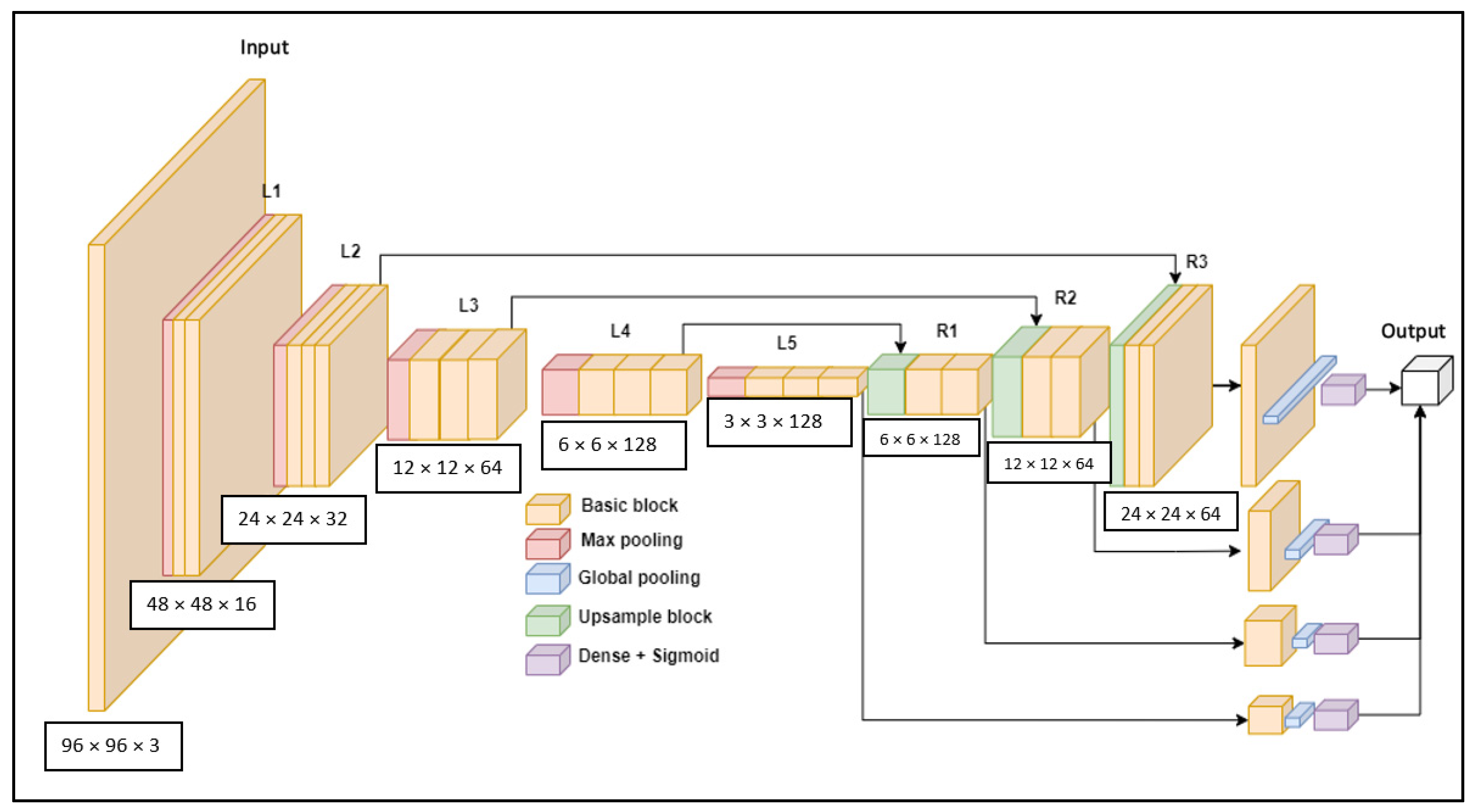
As we stated previously, the U-Net type architecture is currently one of the most popular templates to search for a suitable architecture. It allows you to easily check the signal information of different levels individually and by combining high and low frequency signals in separate levels; in our work, we called it the M-model, shown in Figure 4.

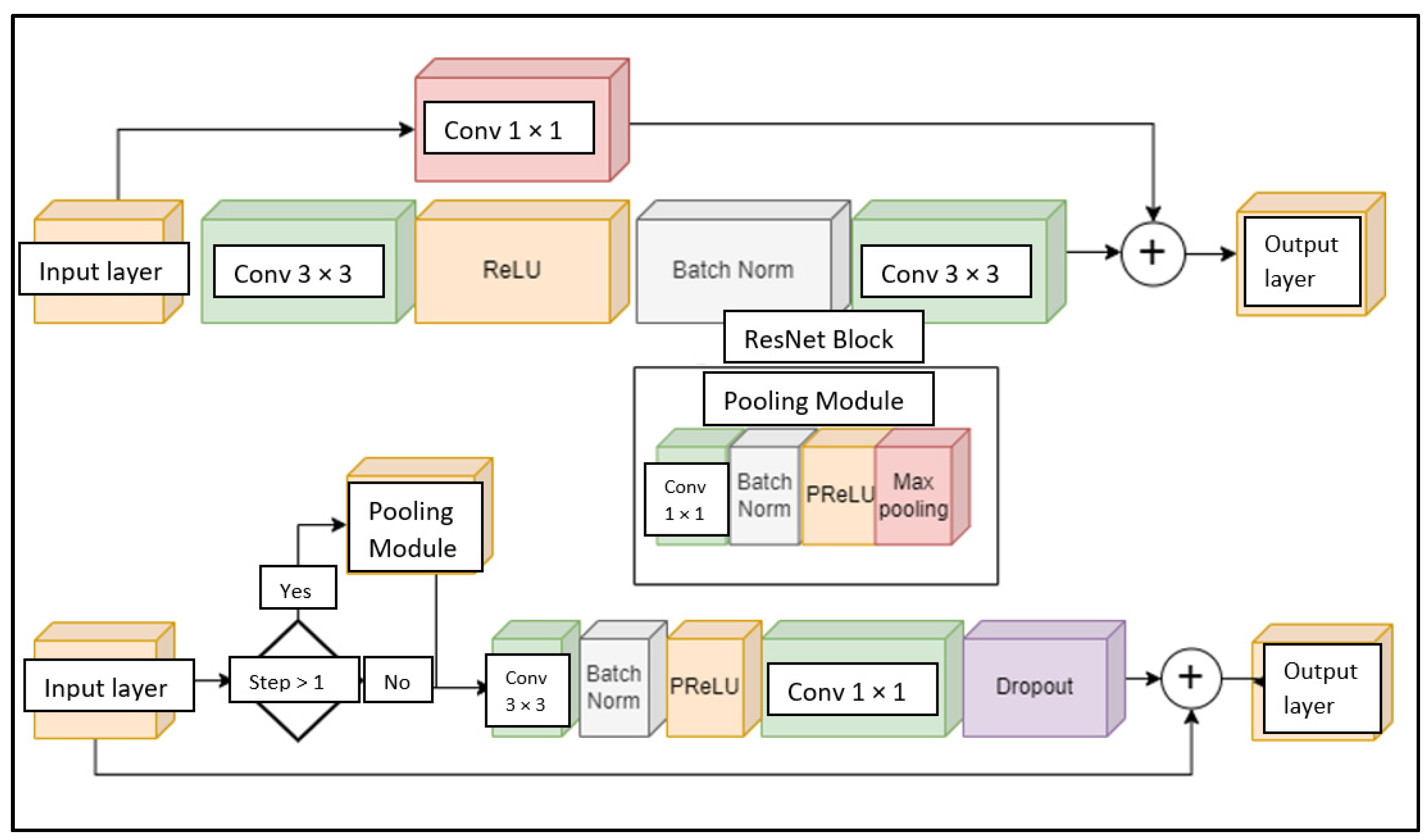
By default, U-Net networks form a complete U-shape—they transmit the entire input signal to the output of the model, which is applicable in this work due to efficiency and the type of task itself. Higher resolution output is usually used for image reproduction or segmentation tasks. In this research, classification was performed from low-resolution images, so the high-resolution output will not be superior. The following changes were made to the intermediate modules of the network structure, that we will call the E-Module, shown in Figure 5. Compared to the commonly used standard ResNet module, the E module was more efficient and faster—two 3 × 3 convolutions were changed to one compressed 3 × 3 convolution and one 1 × 1 convolution, with the same number of channels as the number of input layer channels. Furthermore, the typical ReLU (rectified linear unit) activation was changed to PReLU (parametric rectified linear unit) [75]. In this way, the model will be able to apply the best activation for each layer according to the direction of the gradient. Together with this activation function, it was possible to see the behavior of the model by analyzing the values of the activation coefficients. Finally, a Dropout layer was added at the end of the module, which performs a dual regularization: it reduces the signal bandwidth and allows the dropout factor to be increased to 1 at the end of training to discard supposedly unnecessary parts of the model.

Additionally, the entire network structure was reworked into a dynamic format. Based on the principle of the EfficientNet architecture [76], the rules for growing the width and length of the network were established and adaptive regularization were applied with Equations (5)–(9) shown below:

• Number of filters (5):

$$\mathrm{Number}\mathrm{of}\mathrm{filters}=max\left(16,\frac{f\cdot s\cdot F}{h\cdot 2}\right)\cdot g$$

(5)

• Number of blocks (6):

$$\mathrm{Number}\mathrm{of}\mathrm{blocks}= max\left(2, \frac{\mathrm{Number}\mathrm{of}\mathrm{filters}}{64}\right)$$

(6)

• Exclusion factor (7):

$$\mathrm{Exclusion}\mathrm{factor}=max\left(0.05,\frac{\mathrm{Number}\mathrm{of}\mathrm{filters}}{m/2}\right)$$

(7)

• L2 regularization (8):

  $$\mathrm{L}2\mathrm{regularization}=1\times e-5+\frac{f}{8}\times 0.0001$$

  (8)

  where f is the base number of filters, F is the filter multiplier, s is the filter multiplier, h is the height of the network in pixels, g is the number of convolutional groups of the network. The number of blocks indicates how many internal blocks will make up the mesh module after each decrease or increase in height and width of the mesh. Exclusion factor—indicates how many neurons will be turned off in percentage in each block, where m indicates the maximum possible number of filters. The L2 regularization [77,78] specifies the value of the L2 regularization constant for all network convolutions.

To understand whether all the changes made to the model gave advantages compared to ResNet50 or DenseNet121 models, the following experiments were performed. According to the already presented formula for changing the structure of the model, three sizes for f were selected: 8, 16, 32. Sizing allows us to see the areas where the network performs too poorly, overlearns, and where it performs optimally. It is additionally important to find out from which part of the network the best result can be obtained. Therefore, five output layers were added to the already existing network. Accordingly, we noticed a trend while comparing the results of all outputs. All models gave their best performance from the outputs of L5 and R1. This suggests that using a model with such a structure for this task, a higher resolution not only does not provide additional benefits, but also spoils the result. We can be assured that the most suitable model size for this task is f = 16, as in the first test, models where f = 8 and f = 32 performed worse. Among the model outputs, it can also be seen that higher resolution did not provide enough benefits.

Overall, compared to the first experiment, most of the results have improved, especially the output AUC of L5 has increased from 0.95279 to 0.95341. According to these results, it can be confidently stated that the U-Net type architecture did not provide enough benefits for this task. Moreover, comparing the obtained results with ResNet50 and Densenet121, the new model was already superior in terms of accuracy and learning speed—the new model reached the maximum result in eight epochs, which none of the previously described models was able to do when learning with newly initialized weights. According to the results of the first tests, the U-Net model was modified. We removed the right part of U-Net layers and all intermediate connection, also fixed size multiplier f = 16. Such pruning not only provided speed, but also allowed to gain greater accuracy due to less information reuse, this improved model will be called the MS-model.

4.2. Results

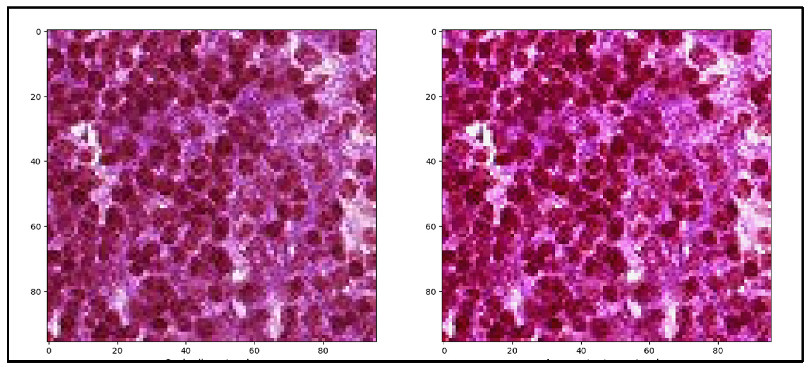
First, we made additional training validation performed on the artificially augmented and non-augmented datasets. The ResNet and DenseNet networks with ImageNet weights were applied for the test. Both models performed with more than 1% greater accuracy with augmented data than with non-augmented data (

Table 1. Learning from zero with testing data set.

	AUC (Area under the Curve)
Model	Using Augmentation	Not Using Augmentation
ResNet50	0.95001	0.93988
DenseNet121	0.95511	0.93780

). It can be assumed that these models were too large for such a task and most probably overlearned as a result, however the AUC value on the training data set shown in

Table 2. Learning from zero with learning data set.

	AUC (Area under the Curve)
Model	Using Augmentation	Not Using Augmentation
ResNet50	0.96501	0.99297
DenseNet121	0.98891	0.99971

confirmed this. Without augmentation, the AUC was almost at unity at 0.993, while with augmented data it was only 0.975 with the ResNet50 model. Although retraining has occurred, the results show that the data generated for training was fine, and the selected augmentations were useful.

After making sure that the training environment and data were correct and everything was working as it should, further analysis was performed. Each selected model was trained twice. First, using ImageNet weights and then applying Xavier weights with initialization according to the training protocol, results are shown in

Table 3. Model architectures analysis results.

	AUC (Area under the Curve)
Model	ImageNet Weights	Xavier Initialization Weights
DenseNet121	0.95672	0.94560
ResNet50	0.95078	0.94380
ResNet50 V2	0.95078	0.94380
MobileNetV1	0.94954	0.93855
MobileNetV2	0.95065	0.95395
Inception	0.94697	0.94608
EfficientNetB0	0.95121	0.94608
EfficientNetB1	0.93876	0.94608
EfficientNetB0 V2	0.94570	0.75981
EfficientNetB1 V2	0.94287	0.79871

.

Comparing with ImageNet weights, DenseNet achieved the best result. According to the learning graph, it exceeded the AUC value of 0.95 after only two epochs. The next best was ResNet50, although it did not show the second result according to the table, but it also exceeded the AUC value of 0.95 after two epochs. Collectively, this means that these two architectures were the most suitable for this task. Furthermore, the ResNetV1 and ResNetV2 models excelled the most. Although their results were not the best, they exceeded 0.94 AUC in just five epochs. This shows that the ResNet-type blocks and persistent connections were well suited for this task due to their fine gradient feedback.

A new training session was performed with the trimmed model called the MS-model. Two tests were selected. The first was by extending the training using the best weights, as shown in

Table 4. MS-model results. New initialization indicates that the model weights were generated by Xavier initialization from a newly chosen random point.

Learning Iteration	AUC
Reusing weights	0.95501
New initialization 1	0.95498
New initialization 2	0.95508
New initialization 3	0.95505

and gave better results after reusing weights. As the original structure of the network remained the same, weights could easily be transferred from one network to another. The second was to train the same network with ever new weights initialization.

A popular way to get a better result is to change the optimization algorithm. Although all training was done with the SGD optimizer, which should potentially be the best for this problem, other methods could potentially find a better solution simply because of the difference in the optimization Hyper parameters. As a result, shown in

Table 5. Comparison of optimization methods.

Learning Iteration	AUC
SGD	0.95510
Adam	0.95475
AdamW	0.95515
Ranger	0.95500

, we learned that of several optimizers, the best result was achieved with the AdamW optimizer.

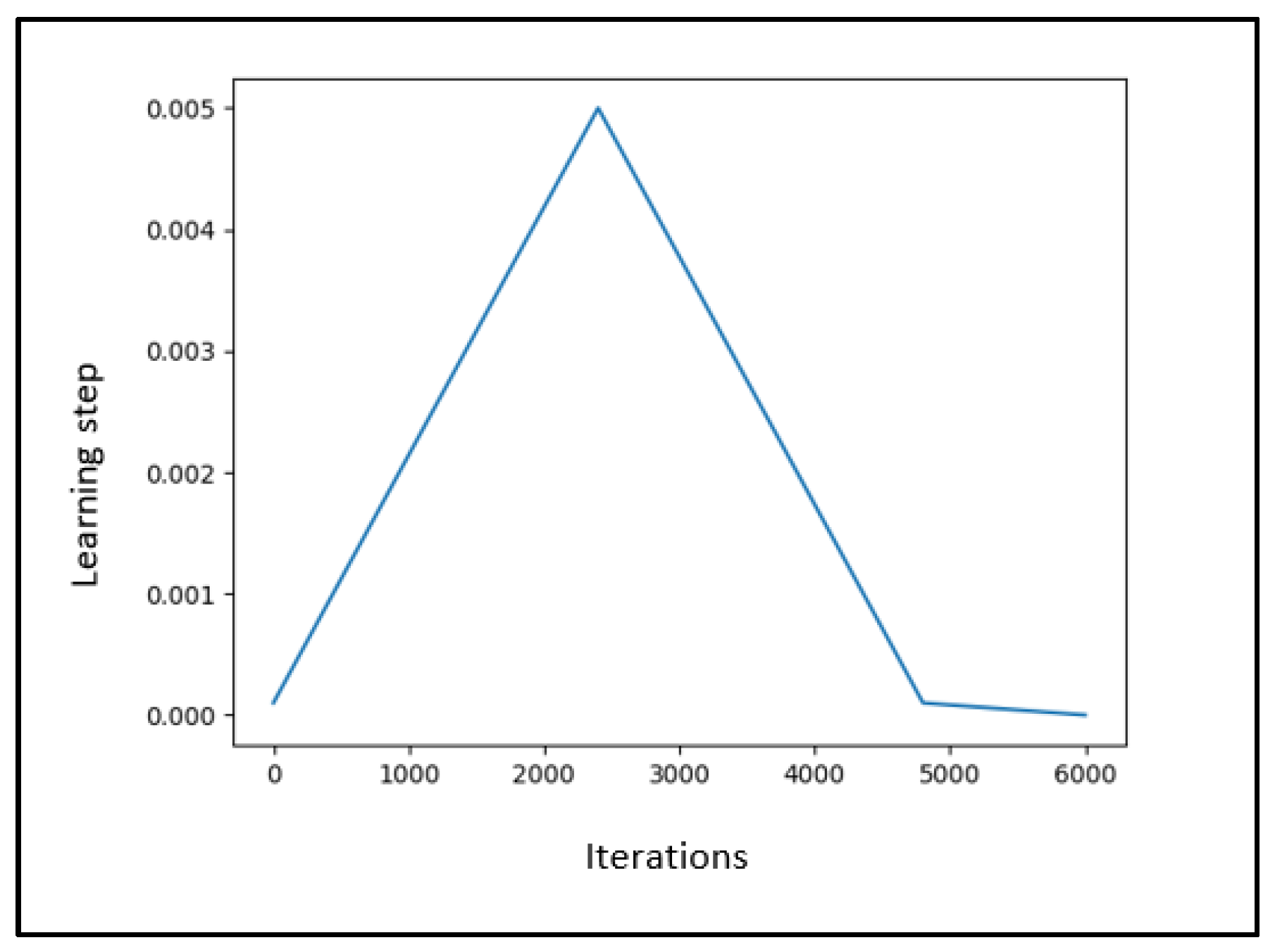
Based on the results of the last test that adding more regularization is better, changes were made to the model and training code. The L2 regularization of the convolutional weights used so far was increased to 1 × 10⁻⁴, and the learning frequency cycle used in the SGD optimizer was converted to cosine. As expected, this teaching principle worked very well. After the fifth iteration, we managed to achieve an AUC of 0.95911, which was almost 0.4% better than the last best model trained with the AdamW optimizer.

In addition to that, we added the TTA [79,80] method, as the training data were adjusted very flexibly—we selected certain featuring: color channel change, vertical flip, horizontal flip, rotate −90 degrees, rotate +90 degrees, lighten the image by 5%, darken the image by 25%; unfortunately, the individually processed images results gained only 0.9590 AUC.

Another approach that did not require model retraining, reengineering, or other changes was model ensemble. This can be done in several ways. We proposed two methods for it. The first one, which combines the outputs of the different models according to the arithmetic mean and returns a single result, and the next one, which combines the weights of the different models into one common list of weight matrices.

5. Discussion

After all strategies and methods, we observed that different training optimizers, more heavily augmented data, learning step graph, or even a well-chosen learning starting point of the model, all influence the overall result when using them combined in an ensemble; it can be argued that the models or weights will converge if their individual performance does not overlap. This means that the models must make different errors among themselves. Therefore, it is obvious that by combining the ensemble methods of the last two experiments, it will be possible to achieve even higher accuracy.

It can be seen in

Table 6. Summary of results. The difference column represents the AUC difference between the type and the first starting point in DenseNet121.

	AUC (Area under the Curve)
Ensemble Type	AUC	Difference
DenseNet121	0.95672	-
M-model training 5 outputs together	0.95405	−0.267%
M-model training 5 outputs separately	0.95491	−0.1891%
MS-model	0.95508	−0.164%
MS-model with AdamW	0.95515	−0.157%
MS-model with repeated training	0.95911	0.239%
MS-model TTA	0.96870	1.198%
MS-model ensemble	0.96592	0.920%
MS-model connecting weights	0.96240	0.568%
TTA + weights and models ensemble	0.96922	1.250%
MS-model after corrections	0.96147	0.475%
MS-model after corrections with repeated training	0.96675	1.003%
Group of ensembles from all experiments	0.96977	1.305%
Optimized ensemble based on the best model	0.97673	2.001%

that all used methods are models that lead our MS-model to be improved from 0.95918 to 0.96675 AUC.

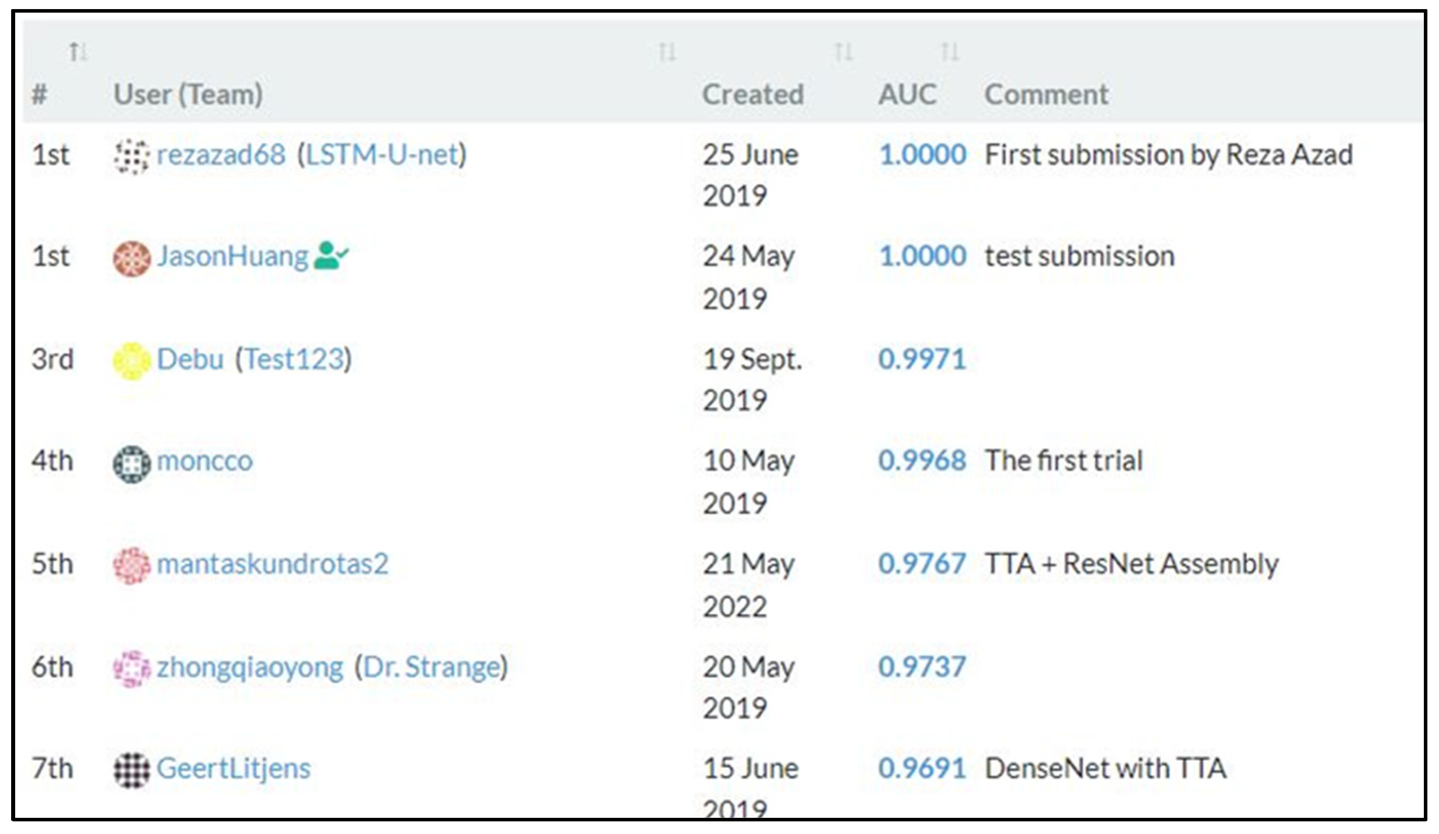
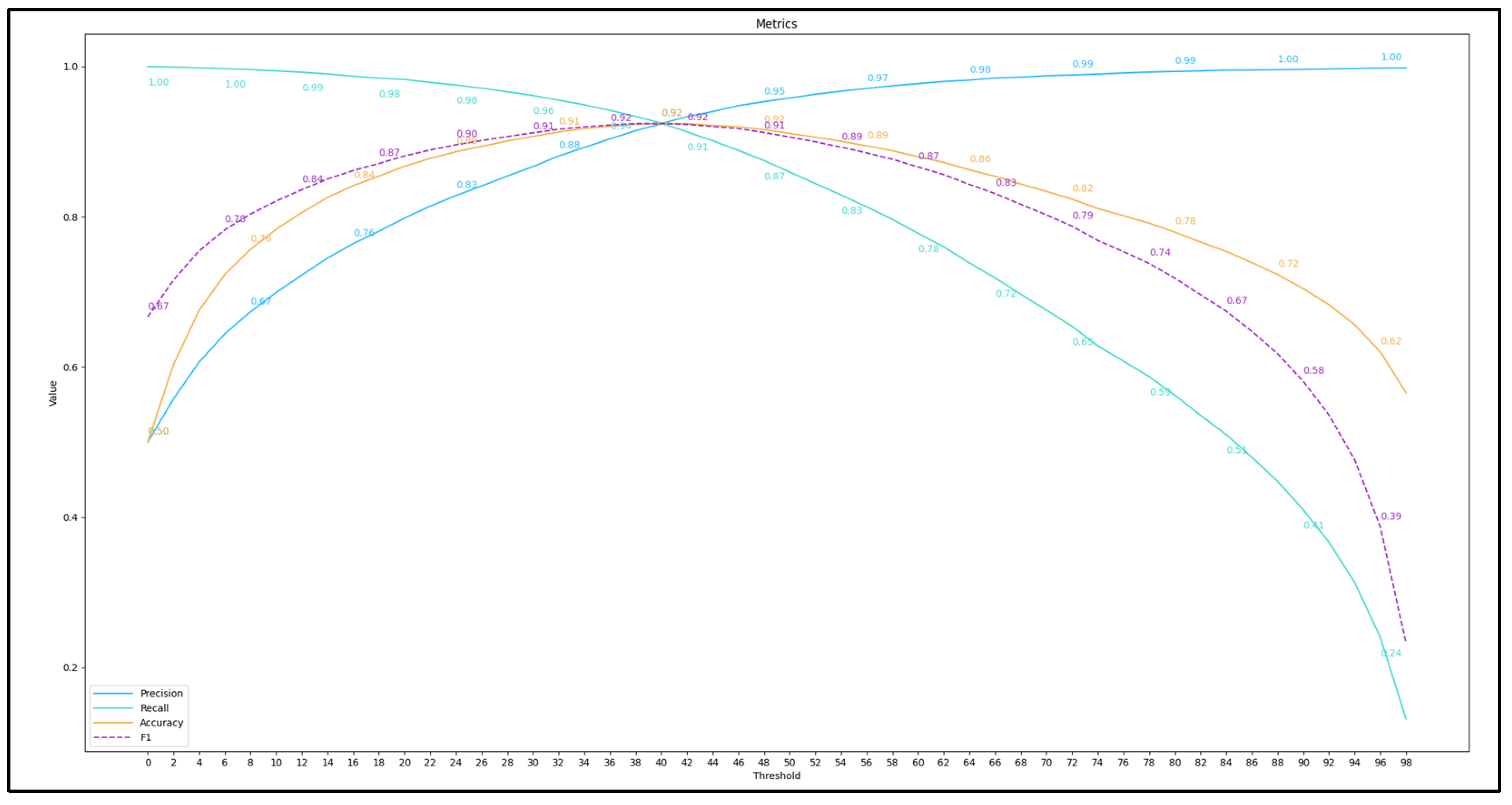
To sum up, it can be stated that artificial neural networks are able to distinguish tissue areas affected by cancer quite well. The developed MS-model is more accurate and faster than most of the models presented in the “Patch Chameleon” standings as shown in Figure 6. It can be said that such accuracy was most influenced by the effective architecture of the neural network and research on combining and assembling models. 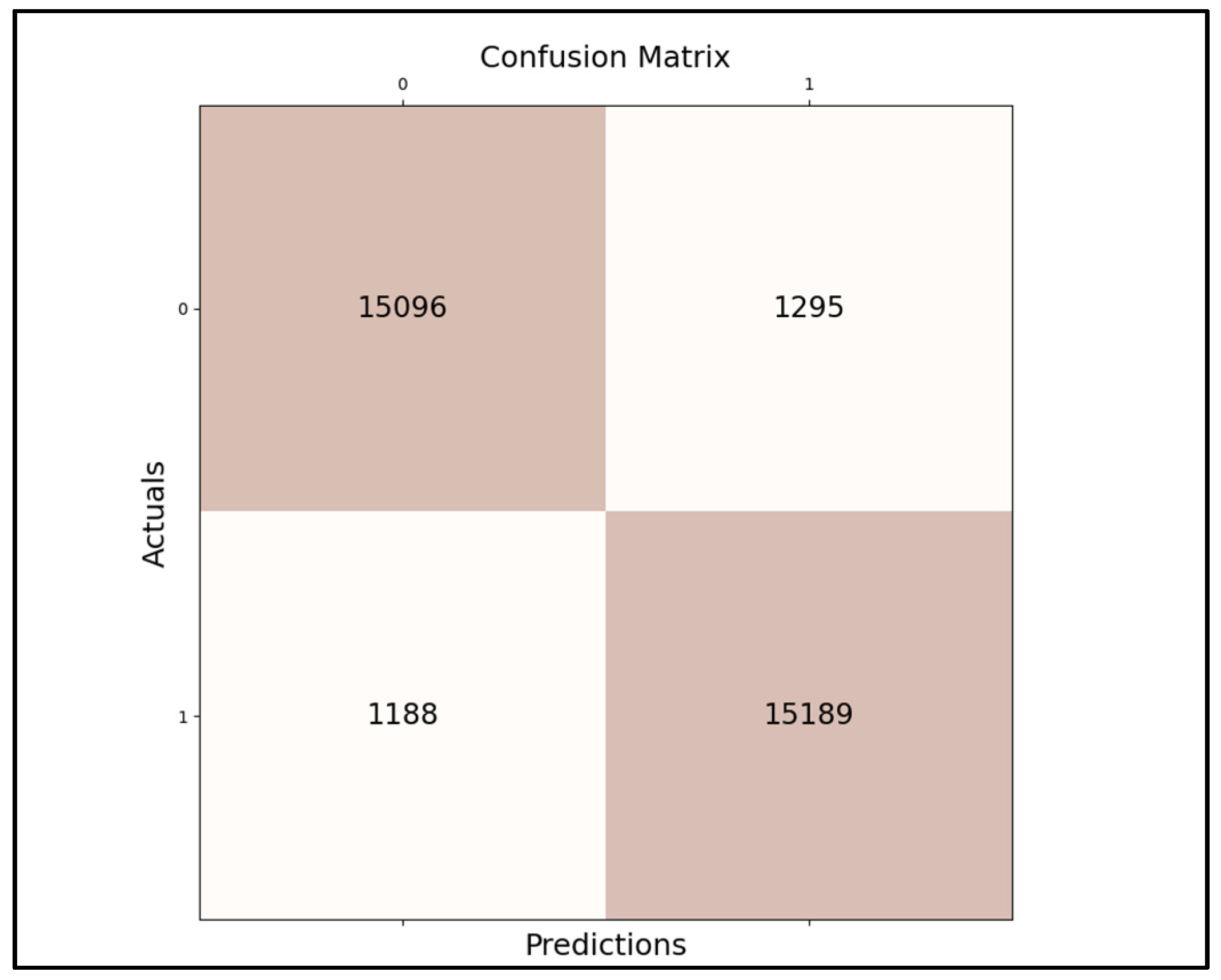As shown in Figure 7, we have reached a maximum F1 score of 0.924 with a threshold of 0.393; this score measured on our last best model’s accuracy (that is evaluated from precision and recall), as long as the confusion matrix is that shown in Figure 8, giving us a result of meaning how many times our best model gave us correct predictions: true positives—15,096, true negatives—15,189, false negatives—1295, and false positives—1188. According to experiments, even with less-than-ideally prepared training data, the last ensemble method managed to exceed 0.9691 AUC.

6. Conclusions

In this work, we proposed to use ML and different neural network techniques to find a solution to WSIs histopathological data analysis. Our extensive experiments showed that the application of artificial deep neural networks for the classification of medical images, compared to other classical methods, are superior in almost all criteria. First, the CNN generalize well and perform similarly well on unseen data, even with additional constraints. From the obtained experiments, the AUC difference between the training and testing datasets was about one percent. Second, these models were highly flexible, allowing the size and architecture of the model to be experimentally tailored to the type of task. Using the M-model in several training iterations, we managed to reduce the model size by almost twice and increase the accuracy from 0.95491 to 0.95515 AUC. Third, when properly trained, convolutional models perform well on groups of various sizes. The result increased to 0.96870 with the TTA method, and 0.96977 with the addition of the multi-model ensemble. Fourth, by applying special analysis methods, it was possible to identify the shortcomings of the models and correct them. After finding that excessive and inappropriate image augmentation was detrimental to learning, a correction of the image processing parameters was sufficient to increase the AUC by almost 0.3%. Moreover, after additional training data preparation, the result of the individual model increased to 0.96664 AUC.

Due to the complexity of histopathological images, current image classification methods still lack accuracy and stability, and even the final model ensemble result of 0.97673 was not sufficient for the system to work autonomously. The results are too unpredictable, so this type of system can only be used as a guide as an image analysis tool for the physician.

Nevertheless, even such an achievement is important—it is a step closer to the ideal accuracy that would exceed human resolution.

In future work, not only another optimizing, and DNN techniques and architectures, but also imaging improving unsupervised methods could be used to gain best accurate results that further diagnostics tools for faster and more accurate cancer detection in histopathology imaging.