A Biologically Inspired Self-Organizing Underwater Sensor Network

Abstract

Wireless underwater sensor networks have various applications—such as ocean exploration and deep-sea disaster monitoring—making them a hot topic in the research field. To cover a larger area and gather more-precise information, building large-scale underwater sensor networks has become a trend. In such networks, acoustic signals are used to transmit messages in an underwater environment. Their features of low speed and narrow bandwidth make media access control (MAC) protocols unsuitable for radio communications. Furthermore, a network consists of a large number of randomly deployed nodes, making it impossible to pre-define an optimized routing table or assign a central controller to coordinate the message propagation process. Thus, optimized routing should emerge via interaction among individual nodes in the network. To address these challenges, in this paper we propose a communication coordinator under the time division multiple access (TDMA) framework. Each node in the network is equipped with such a coordinator so that messages in the network can be sent following the shortest path in a self-organized way. The coordinator consists of a slot distributor and a forwarding guide. With the slot distributor, nodes in the sensor network occupy proper communication slots and the network finally converges to the state without communication collision. This is achieved with a set of ecological niche- and pheromone-inspired laws, which encourage nodes to occupy slots that can decrease the waiting time for a node to send a message packet while weakening the enthusiasm for a node to occupy the slots that it fails to occupy several times. With the forwarding guide, a node can send the message packet to the best successor node so that the message packet can be sent to the base station along the shortest path. It has been proven that the laws in the forwarding guide are equivalent to the Dijkstra Algorithm. Simulation experiment results indicate that with our coordinator, the network can converge to the state without collision using fewer coordination messages. In addition, the time needed to send a message to the destination is shorter than that of the classical Aloha protocol.

1. Introduction

Underwater sensor networks are important tools in the marine environment. They can be applied to gather oceanography data, track marine animals, monitor the pollution of the environment, and defend harbors from intruders [1,2]. In an emergency, a large number of sensor nodes can be deployed by planes or ships to cover a large arena, which forms a large-scale wireless underwater sensor network. Due to the ability to deploy and monitor large areas in a short period of time, such sensor networks have become a hot topic in the research field.

A large-scale wireless underwater sensor network has the following features:

• Communication among nodes is achieved via acoustic communication. Radio signals attenuate fast in the water, and underwater laser communication is unreliable under the disturbance of water flow. As a result, acoustic communication becomes the only choice for wireless communication in wireless underwater sensor networks.
• The communication routing should emerge in a self-organized way. In large-scale wireless underwater sensor networks, it is expected that a message can reach its destination node as soon as possible. However, as nodes are deployed randomly, users are unable to set a routing table for each node before deployment. The communication constraints of acoustic communication make it impossible to assign a central coordinator to control the communication process of the whole network. As a result, we can only seek a self-organized way to coordinate communication in the network.
• Communication collision should be avoided as much as possible. For underwater acoustic communication, if one node hears multiple signals at the same time, it is unable to parse the information included in any signal. The same thing happens when it hears a signal while speaking at the same time. These phenomena are called communication collisions. When a communication collision occurs, the sender node needs to resend the message, extending the time for a message to reach its destination.

The aforementioned features make currently available self-organizing schemes not applicable in an underwater environment. For example, under a time division multiple access (TDMA) framework [3] there are two kinds of schemes to coordinate the self-organizing communication process for radio communication. The first type of scheme is developed following the idea of “collision detection and resend”, such as the famous Aloha protocol. In these schemes, a node tries to send a message in a slot, and once a collision happens, it will resend the message later in another slot. For radio communication, each slot lasts only several microseconds or less. Thus, it can endure wasting time. However, for acoustic communication, each slot lasts several seconds, and thus wasting time is unaffordable, making these protocols an unfavorable choice. Other schemes have been developed following the idea of “constructing an optimized routing table via communication”, such as the method proposed in [4]. In these schemes, an extra message needs to be conveyed to coordinate the communication. Taking the method in [4] as an example, nodes need to send the IDs of all their neighbors, their second-order neighbors (i.e., neighbors’ neighbors), and slots occupied by each of these nodes. As a result, a node can obtain information about all its first- and second-order neighbors to decide which slot it should occupy. The drawback of this method is that the extra data occupy much communication capability for acoustic communication. Consequently, a method to coordinate the acoustic communication process in a large-scale wireless underwater sensor network is necessary.

In this paper, we propose a coordinator to coordinate communication for a large-scale wireless underwater sensor network. It is developed under the TDMA framework and consists of a slot distributor and a forwarding guide. The slot distributor is used to determine which slot the current node should occupy. An ecological niche- and virtual pheromone-inspired scheme is used to encourage the current slot to occupy more slots, while a collision resolver eliminates conflicts when multiple nodes try to occupy the same slot. Finally, the network can converge to a state where no communication collisions exist. The forwarding guide then decides how to transmit a message packet to the base station promptly. This is achieved by defining a metric called expected wait, which indicates the expectation of the wait-time needed before a message packet is out, with the message packet received at a random time. Based on this metric, the forwarding guide can provide the ID of the next node that should relay the message so that the message can travel to the base station following the shortest path. The effectiveness of this coordinator has been proved with mathematical analysis and simulation experiments.

The rest of this paper is organized as follows. In Section 2, the works related to this paper are introduced. In Section 3, we introduce the problem and provide the framework of the communication coordinator of this paper. Then, in Section 4 and Section 5, the components of the coordinator are introduced in detail, with Section 4 providing the slot distributor and Section 5 giving the forwarding guide. Then, in Section 6, the performance of the method is verified with simulation experiments. Finally, we conclude this paper in Section 7.

2. Related Work

Underwater communication plays an essential role in underwater wireless sensor networks (UWSNs) [5]. To meet increasing exploitation demands of submarine resources, various underwater communication devices and methods have been proposed [6,7]. The technologies for the transmission of wireless underwater communication can be classified into three categories, i.e., radio frequency (RF) communication, optical communication, and acoustic communication [8]. Each technology is reviewed in detail in the following sections.

RF communication technology is unsuitable for underwater environments since the high conductivity of seawater severely affects the propagation of electromagnetic waves [9]. Che et al. [10] have found that RF communication can be used in shallow-water environments. However, RF communication technology still suffers from many limitations such as serious signal interference by environmental noise [11] and huge energy loss in the propagation process [10]. Studies have proved that the RF data rate varies from 1 to 10 Mbps [12], and the communication distances are only a few meters [13].

Compared to RF technology, optical communication technology exhibits a better data rate. Hanson and Radic revealed that the data rate of optical communication reached up to 1 Gbps [14]. However, the reliable communication distance is only tens of meters, from about 2 to 25 m [15]. Zhang et al. found that the attenuation of optical signals of different frequencies underwater varies, and the blue–green optical signal has a smaller propagation attenuation [16,17]. Moreover, the attenuation and interference of optical signals are also affected by different water environments. Therefore, optical communication is more disadvantageous to underwater communication than RF communication [18].

Acoustic communication possesses more advantages than the other two technologies for underwater environments [6], and its communication distance can reach several kilometers [19]. Due to the speed difference between sound and electromagnetic waves [20], there exist three main losses—spreading loss, absorption loss, and scattering loss—that affect the propagation distance of acoustic waves [21]. Li et al. show that the data rate of sound waves is only 0.6 to 50 Kbps [22]. To address the problem of low acoustic wave propagation rates and the increasing number of deployed devices, wireless sensor networks (WSNs) [5] have become an efficient tool in the underwater environment.

WSNs, however, suffer from serious problems such as resource allocation, interference management, anti-blocking, and deafness [5]. Zhou et al. used MAC protocol, which focuses on improving the performance and efficiency of communication [23], in their study to solve such problems in WSNs [24]. Zhang et al. indicated that it is significant to analyze MAC protocols in the study of WSNs [25]. Han et al. found that in WSNs, MAC protocols operate at the top layer of the physical layer [26]. Meanwhile, MAC protocols always consider energy efficiency [27]. All these elements are crucial for the lifetime and efficient operation of WSNs.

Nonetheless, the MAC protocols used in terrestrial wireless sensor networks (TWSNs) are unsuitable for UWSNs because these MAC protocols exhibit low bandwidth, low throughput, high energy consumption, and high propagation delay [28,29,30]. Time synchronization in UWSNs is another difficult factor because effective operation cannot be confirmed between sensor nodes and higher propagation delay [31], which leads to too many re-transmissions and collisions in UWSNs [32]. There exist many MAC protocols used for UWSNs, such as OFDMAC, UW-OFDMAC, ED-MAC, and DL-MAC [23]. However, they cannot meet all the requirements in different underwater environments. To conclude, it is imperative to leverage a variety of methods to improve the MAC protocol in acoustic communication, such as using a learning machine to make sensors predict possible scenarios in real time [33]; studying for cross-layer design can improve the efficiency of MAC protocols [34].

3. Problem Statement and Solution

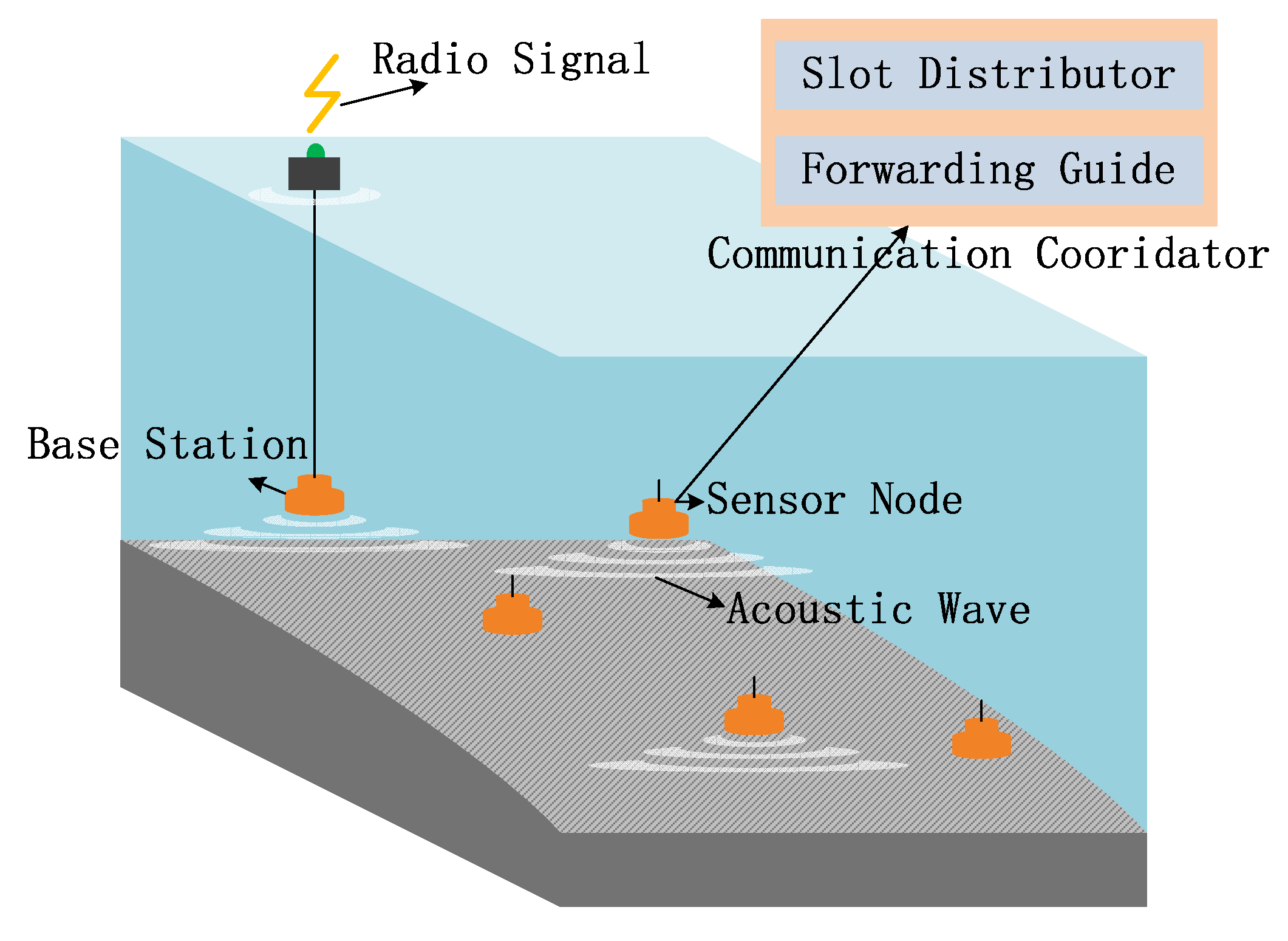
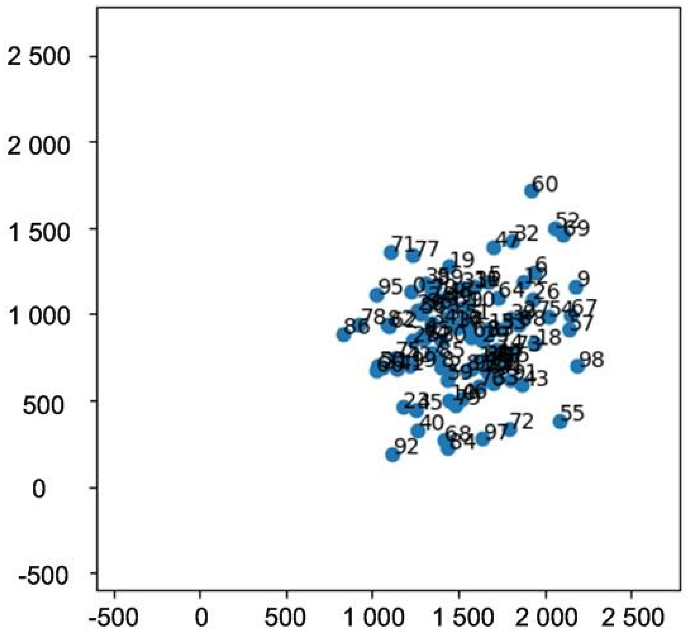
The problem that we seek to solve in this paper is to obtain a scheme to coordinate the wireless communication of nodes in a large-scale wireless underwater sensor network. As shown in Figure 1, N sensor nodes are randomly deployed into the area of interest by a ship or a plane, where N can reach tens, hundreds, or thousands. Once deployed, these nodes sink underwater and float at a certain depth, collecting information within their detection ranges. As all nodes are underwater, they can only communicate with each other via acoustic signals, with the communication range being r.

Here it is assumed that a high-frequency acoustic signal is adopted, and thus r is of hundreds of meters, with communication speed being several Kbps. Among these nodes, there is a special node called a base station that is connected to an antenna floating at the surface of the water. Thus, the data collected by other nodes are transmitted to the base station node jump-by-jump via acoustic communication and are finally sent to the control center via radio signals by the base station node. Consequently, even though nodes can be deployed randomly, they must form a connected graph (treating nodes as vertexes and assigning an edge between a pair of nodes whose distance is less than r), otherwise messages from some nodes are unable to reach the base station.

With acoustic communication, if one node hears multiple signals at the same time, or it hears signals while speaking at the same time, the node is unable to parse the information contained in the signal. In this paper, this phenomenon is called communication collision.

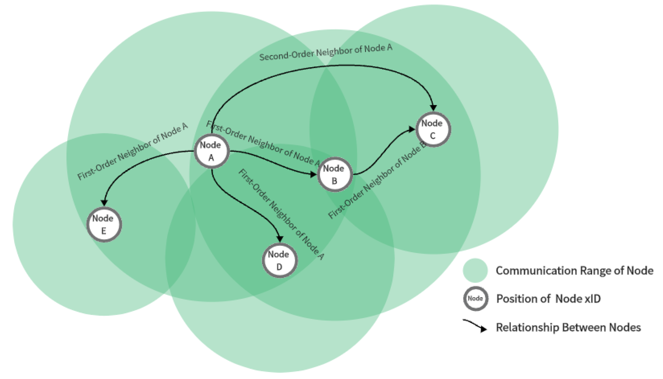
To define this concept formally, let us define $dis(i,j)$ as the distance between Nodes i and j. If $dis(i,j)<r,i\ne j$, we call Node j the first-order neighbor of Node i, and vice versa. Further, if there exists Node k that satisfies:

$$dis(i,j)<r\wedge dis(j,k)<r\wedge dis(i,k)>r,$$

then we call Node k the second-order neighbor of Node i. Intuitively, a second-order neighbor represents a neighbor’s neighbor. Note that the neighbor relationship is defined based on the relative position of nodes. If the nodes’ positions change, the neighbor relationship may also change. In the following sections, variables defined for first-order neighbors are indicated with subscript ${}_{1\text{-}neighbor}$ and for second-order neighbors with subscript ${}_{2\text{-}neighbor}$. The subscript ${}_{12\text{-}neighbor}$ indicates variables with both first-order neighbors and second-order neighbors. The definition of the neighborhood is shown in Figure 2.

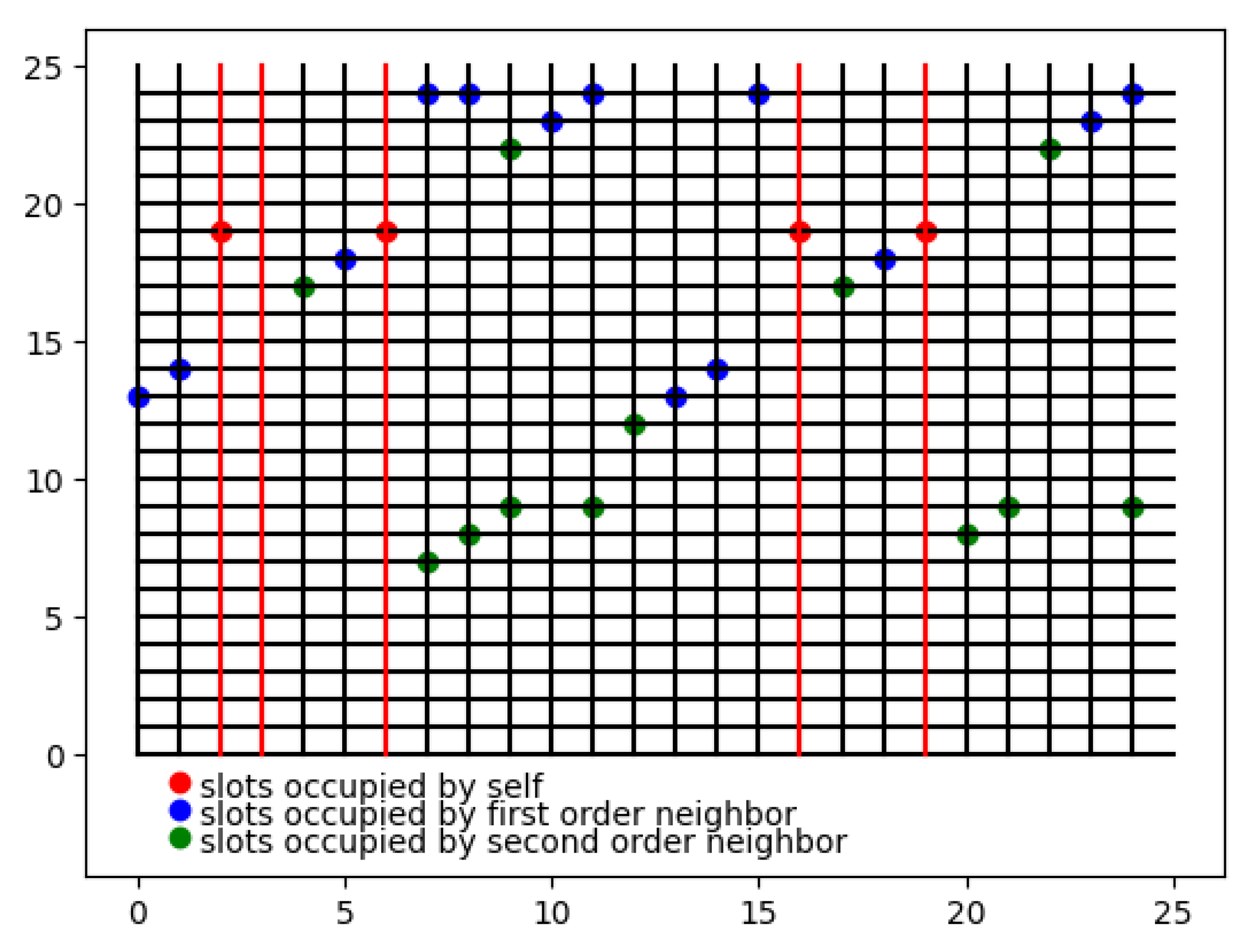
According to the definition of communication collision and neighborhood relationship, it can be obtained that for Node i, let $S_{1\text{-}neighbor}$ be the set of all its first-order neighbors and $S_{2\text{-}neighbor}$ be the set of all its second-order neighbors. If the following conditions are satisfied, no communication collision will happen on Node i. The conditions are:

• At most one member in $S_{1\text{-}neighbor}\cup i$ speaks at the same time.
• When i speaks, no node in $S_{2\text{-}neighbor}$ speaks.

From the conditions above, we can conclude that for the whole network, if no node speaks at the same time as any of its first-order neighbors or second-order neighbors, then no communication collision exists in the network.

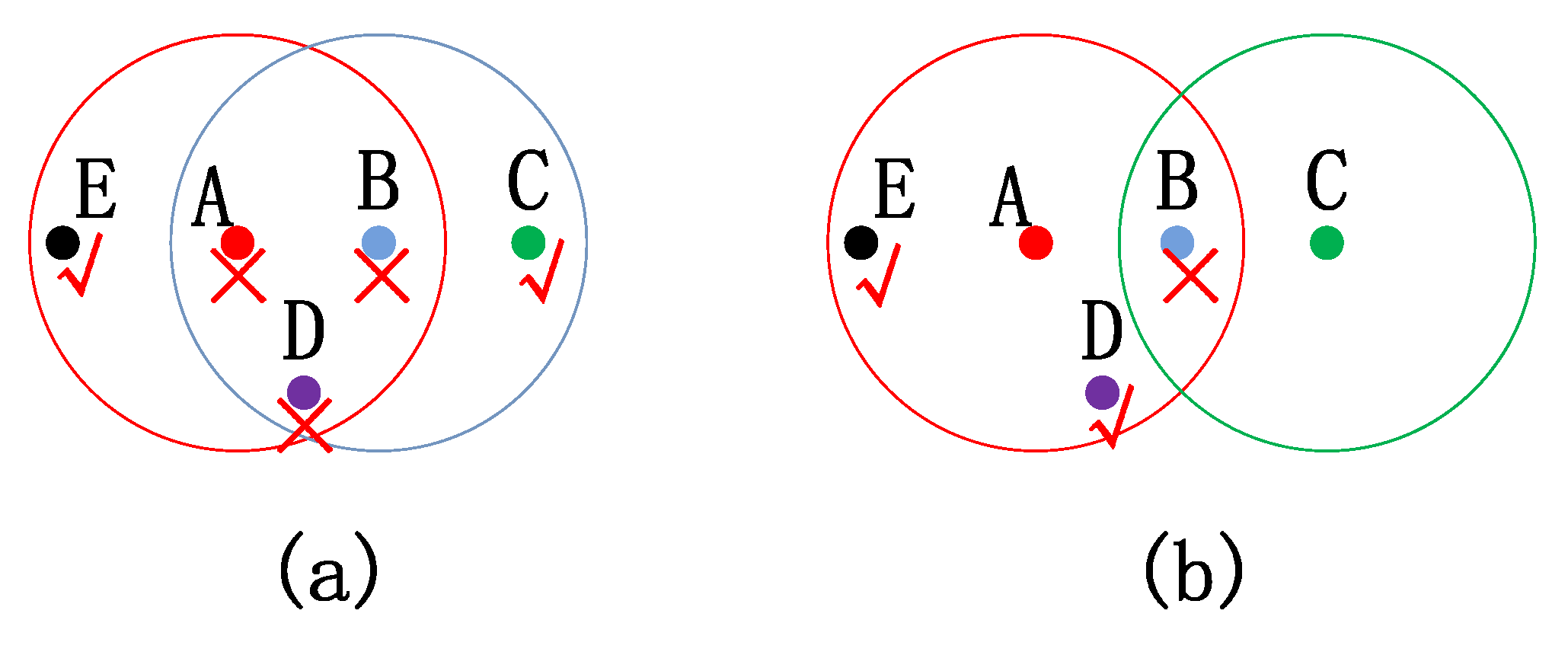
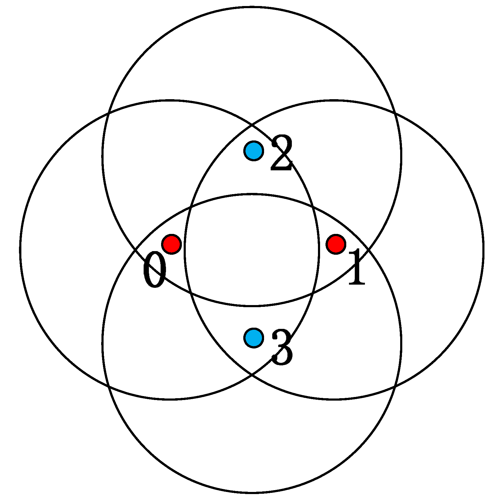
In the network, a node can detect two types of collisions as follows

• Collision with its first-order neighbor. When a node speaks at the same time as its first-order neighbors, it is able to detect this collision.
• Collision of multiple first-order neighbors. For a node, when multiple of its first-order neighbors speak at the same time, this node is able to detect this collision. However, if the speaking neighbors themselves are not first-order neighbors to each other (i.e., they are second-order neighbors to each other), then these speaking neighbors are unable to detect this collision.

The collision situations are shown in Figure 3.

For the sensor network, it is expected that messages can be sent from any node to its destination node (i.e., the base station) successfully and as fast as possible. It is best if no collision happens in the network. As nodes are randomly deployed and the number of nodes is large, the communication process should emerge in a self-organized way. To achieve this goal, we propose a communication coordinator in this paper. As shown in Figure 1, each node in the network is equipped with the same coordinator.

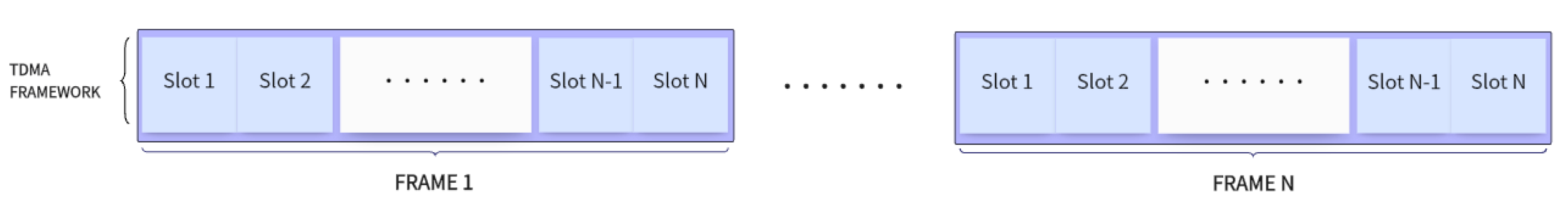
The coordinator is developed under a fixed-length TDMA framework as illustrated in Figure 4. In the framework, time is divided into a sequence of communication frames, with each frame consisting of N communication slots, the same as the number of nodes in the network. Each slot is assigned an ID sequentially. Thus, for each node, there exists a slot whose ID is the same as the ID of this node. The slot is called the identical slot of the node.

The TDMA framework is adopted because it can help extend the working environment of our method. The speed of an acoustic signal is affected by several factors, such as the water temperature, water pressure, and so on. Thus, in different environments the communication speed is not the same. Under the TDMA framework, the minimum time unit for communication is a communication slot. If we set the communication slot properly, i.e., within the duration of a slot, all nodes within the range can finish the receiving process (the time for signal traveling and data parsing) under the worst situation, and the method can always work under different conditions. In this paper, high-frequency communication devices are adopted, so the communication range is several hundred meters, and the communication speed is several Kbps (generally 1–2 Kbps). As information can be parsed fast, the time for communication is mainly spent on signal traveling. Considering the speed of an acoustic signal in water is around 1500 m/s, if the size of each message packet is set to 1–2 Kbit, setting a slot to be several seconds is enough for all nodes within the communication range of the sender node to receive the signal and parse the data. As the slots are set long enough, we can ignore the impact caused by the working conditions.

Based on this framework, a communication coordinator is proposed. The coordinator consists of a slot distributor and a forwarding guide. Via interaction with neighbors, the slot distributor provides a list corresponding to the communication frame indicating the nodes occupied by the current slot. Details of the slot distributor will be introduced in Section 4, where we explain how a node occupies proper slots and the network can converge to the state without collision. When a node receives a message packet, the forwarding guide decides if it should be ignored or sent to a certain neighbor. Details are in Section 5, where we prove the message packet can be sent to its destination along the path with the shortest expected wait.

With the communication coordinator, the message packet sent by a node contains the following information:

$$(i{d}_{self},S_{1\text{-}neighbor},S_{abandon},c_{self},i{d}_{next},S_{msg})$$

with $i{d}_{self}$ indicating the ID of the speaker, and $S_{1\text{-}neighbor}$ containing the IDs of the speaker’s first-order neighbors. $S_{abandon}$ is a set generated by the collision resolver. On receiving $S_{abandon}$, a node needs to abandon the occupation of slots in this set except for its identical slot. The variable $c_{self}$ indicates the cost of the current node to send the message to the base station, whose initial value is ∞ unless the node itself is the base station (then, the value becomes 0), and $i{d}_{next}$ indicates the ID of the next node that should relay the message packet so that the packet can be sent to the base station jump-by-jump. The initial value of $i{d}_{next}$ is $-1$, indicating that the node cannot decide on a successor. $S_{msg}$ contains the data collected by the sensor that need to be sent to the base station.

The message packet a node receives contains the same information. To avoid confusion, in the rest of this paper, we use superscript ${}^{sender}$ to mark the information of the sender, so the received message packet is written as

$$(i{d}_{self}^{sender},S_{1\text{-}neighbor}^{sender},S_{abandon}^{sender},c_{self}^{sender},i{d}_{next}^{sender},S_{msg}^{sender}).$$

For readers to better understand this paper, the definitions of key variables are summarized in

Table 1. Variable definitions.

Variable	Definition
N	the number of sensor nodes and length of frame
r	the communication range
$c_{self}$	the cost for the current node to send a message to the base station
$S_{1\text{-}neighbor}$	the set that contains first-order neighbors
$S_{2\text{-}neighbor}$	the set that contains second-order neighbors
$S_{12\text{-}neighbor}$	the set that contains all first- and second-order neighbors
$S_{abandon}$	the set that contains slots that should be abandoned
$i{d}_{self}$	ID of the node that sends the message
$i{d}_{next}$	the next node ID that should relay the message
$S_{msg}$	the set that contains messages to be sent
$L_f$	communication table
$t_{exp}$	expected wait

.

4. Ecological Niche-Inspired Slot Distributor

With the slot distributor, each node can obtain a list called the communication table as $L_f=[v_1,v_2,\dots ,v_N]$, with 

$$v_i=\left\{\begin{array}{cc}1& slotiisoccupiedbycurrentnode\\ 0& otherwise\end{array}\right.$$

A node can speak at the slot it occupies. It is expected that with the slot distributor, each node occupies some slots so that the system achieves:

1. No collisions exist in the whole network;

2. All nodes occupy a greater number of slots;

3. The slots occupied by a node are scattered evenly in the frame.

Items 1 and 2 indicate that communication resources can be used efficiently and sufficiently; 3 indicates that when the need of sending a message packet appears at a random time, it will take less time for a node to wait for a slot it can speak to. Or, formally, in this way, the expected wait formally defined in Section 5 can be decreased.

To achieve the above goals, the slot distributor consists of two parts. The distributor inspired by phenomena in an ecological system encourages nodes to occupy more slots, and slots scattered evenly have a higher probability to be occupied. The collision resolver can eliminate collisions generated by the distributor.

4.1. Slot Distributor

An ecological niche describes the ecological role of specie in the ecosystem. Species have different preferences for different resources such as food. Different species living in the same region usually occupy different ecological niches or show different preferences for similar resources. Otherwise, conflicts occur and war among species happens until a winner is generated. This phenomenon inspires us to treat nodes as species and communication slots as resources. Thus, the preferences of nodes for slots can be used to mimic the ecological niche of species. If nodes show different preferences for slots, they are encouraged to occupy slots with different probabilities. As a result, nodes try to occupy more slots, while the chance of collision can be decreased. If the preference is scattered in a way that can guide nodes to occupy slots evenly scattered in the frame, the expected wait can be decreased.

With an ecological niche, nodes are encouraged to occupy slots, which introduces collisions into the sensor network. Even though the chance of a collision can be decreased, it cannot be eliminated with an ecological niche. Therefore, we introduce the phenomenon of pheromone markers. In the wild, animals deploy pheromone markers to transmit messages. For example, ants use pheromone clues to tell their mates the path to food, and wolves use urine to mark the ownership of territory. Wounded fish can use a pheromone to mark the existence of danger in the environment, and others avoid visiting these marked territories. Similarly, if a node fails to occupy a slot, it can deploy a pheromone there. Once the density of the pheromone reaches a threshold, the node stops attempting to occupy the slot. As a result, no more communication collisions are introduced into the sensor network.

Following the above ideas, we propose the ecologically inspired slot distributor shown in Algorithm 1.

As shown in Algorithm 1, initially, all nodes only occupy their identical slots. List $L_{pheromone}$ shows the pheromone density in each slot. Once a robot fails to occupy a slot, it deploys a pheromone there. Once the density reaches a threshold, the robot stops attempting to occupy the slot again. Initially, the pheromone density in each slot is set to a small value, indicating they can all be occupied, as in Line 1. Then, in Line 2, for the first several frames, nodes do not try to occupy slots other than their identical slots. In this stage, no collision exists in the network. When a node receives a message packet, the node can obtain the ID of the sender and the first-order neighbors of the sender from the message packet. Apparently, the sender is a first-order neighbor of the node, and the sender’s first-order neighbors may be the node’s first-order neighbors or second-order neighbors. Thus after the first several frames, all nodes can obtain a set $S_{12\text{-}neighbor}$ containing all their first- and second-order neighbors. Then, a node can calculate its preference for all slots and the preference for all its neighbors. Then the node occupies the slots in which it has a larger preference than those of all its neighbors, as in Line 3 in Algorithm 1.

The preference is calculated as Algorithm 2. An example is shown in Figure 5.

Algorithm 1 Slot distributor

1: Set initial values: $L_f\leftarrow [0,0,\dots ,0]$, $L_f\left(i{d}_{self}\right)\leftarrow 1$, $L_{pheromone}\leftarrow [0,0,\dots ,0]$, $S_{tryOccupy}\leftarrow \varphi$ 2: Wait for several frames to obtain set $S_{12\text{-}neighbor}$ containing IDs of all first and second-order neighbors 3: Calculate ecological preference of self $p_{self}$ and all neighbors $p\left(i\right),i\in S_{12\text{-}neighbor}$, 4: $L_f\left(i\right)\leftarrow 1$ if $p_{self}>p\left(i\right),\forall i\in S_{12\text{-}neighbor}$. 5: while New slot with address=$i{d}_{slot}$ do 6:     if $i{d}_{slot}\in S_{tryOccupy}$ then 7:         delete $i{d}_{slot}$ from $S_{tryOccupy}$ 8:         if  $L_f\left(i{d}_{slot}\right)=1$ then 9:              keep occupying this slot by setting $L_{pheromone}\left(i{d}_{slot}\right)\leftarrow 0$ 10:         else 11:            Increase pheromone density by $L_{pheromone}\left(i{d}_{slot}\right)$. 12:         end if 13:     end if 14:     if $L_f\left(i{d}_{slot}\right)=1\wedge L_{pheromone}\left(i{d}_{slot}\right)<k_{threshold}\wedge random\left(p_{self}\right)<k_{occupy}$ then 15:         Try to occupy this slot: $S_{tryOccupy}\leftarrow S_{tryOccupy}\cup i{d}_{slot}$, $L_f\left(i{d}_{slot}\right)\leftarrow 1$ 16:     end if 17: end while

Algorithm 2 Calculation of preference

1: Treat the frame as a circle, as shown in Figure 5 2: Set the preference of the identical slot as 1 3: Put identical slot in set $S_{assigned}$ 4: while Not all slots have been assigned preferences do 5:     $S_{wait}\leftarrow \varphi$ 6:     for $slo{t}_{start}$ in $S_{assigned}$ do 7:           Search the circle clockwise until find the next slot in $S_{assigned}$, and record this slot as $slo{t}_{end}$ 8:           Find the center slot between $slo{t}_{star}$ and $slo{t}_{end}$, and name it $slo{t}_{center}$. 9:           Calculate the preference of $slo{t}_{center}$ as $p\left(slo{t}_{center}\right)\leftarrow 1/2·min(p\left(slo{t}_{start}\right),p\left(slo{t}_{end}\right))$ 10:         Put $slo{t}_{center}$ into $S_{wait}$ 11:     end for 12:     $S_{assigned}\leftarrow S_{assigned}\cup S_{wait}$ 13: end while

Then, in Line 4, the slot distributor starts to work. At the beginning of a new slot, a node first updates the pheromone in the slot, as in Lines 5–12. If the node tries to occupy a slot recorded in $S_{tryOccupy}$ and the slot is occupied successfully because it is still in $L_f$, the node occupies this slot by setting the pheromone value to 0. If it fails, the pheromone value in this slot is increased and will eventually become larger than the threshold $k_{threshold}$. Then, the node will never try to occupy this slot again. Then, in Lines 13–16, the node checks if it should try to occupy the current slot. If the slot is not in $L_f$ yet but the pheromone density is below the threshold, there is a chance that the node will try to occupy the slot. The chance of a node trying to occupy a slot is related to its preference for the slot. Nodes are encouraged to occupy slots in a more-evenly distributed manner.

As a result, with Algorithm 1, the communication table $L_f$ is updated. The ecological niche encourages nodes to occupy proper slots, while virtual pheromones can weaken the tendency of changing $L_f$, so finally $L_f$ will keep still. Updating of $L_f$ may introduce collisions into the network, which can drastically hinder the communication of the network in the first several frames. A trick to solve this problem is to not call the slot distributor every frame but to call it once every 5–10 frames. Then there will be fewer collisions in the first several frames and $L_f$ can be improved gradually, which can be solved by the collision resolver.

4.2. Collision Resolver

The collision resolver is shown in Algorithm 3. It can update communication table $L_f$ according to the received message. The message packet received contains a set of slots the sender asks its neighbors to abandon as $S_{abandon}^{sender}$. The algorithm also provides $S^{abandon}$, which contains a set of slots that the current node asks its neighbors to abandon.

Each node maintains two lists: $L_{abandon}$ and $L_{record}$. Let $L_{abandon}\left(i\right)$ be the $i^{th}$ element of $L_{abandon}$. Then $L_{abandon}\left(i\right)=1$ indicates the current node should ask its first-order neighbors to abandon slot i. Let $L_{record}\left(i\right)$ be the $i^{th}$ element of $L_{record}$. Then $L_{record}\left(i\right)=k(k\ne 0)$ indicates a current node has broadcast a message at slot k to ask its neighbors to abandon slot i.

In the algorithm, Lines 3–7 describe the behavior of a node at the slot it occupies. It sends a message packet containing $S_{abandon}$ asking its neighbors to abandon slots in $L_{abandon}$ and record to which slot the requirement is sent in $L_{record}$. Lines 8–26 describe the behavior based on the message received. If the current node collides with any of its first-order neighbors, it will abandon the current slot unless the slot is its identical slot, as in Lines 8–12. In Lines 13–22, if multiple first-order neighbors speak at the same time, the current node checks if it has asked neighbors to abandon this slot before according to $L_{record}$. If so, the current node abandons the current slot unless it is its identical slot. Otherwise, the current node records this slot in $L_{abandon}$. In the case that the current node successfully receives a message packet, the node abandons slots in $S_{abandon}^{sender}$ in the message packet except for its identical slot, as in Lines 23–25. Finally, $L_{record}$ is updated in Line 26.

Algorithm 3 Collision resolver

Input: Communication table $L_f$, Communication packet received, contains $S_{abandon}^{sender}$

Output: Update communication $L_f$ and generate $S_{abandon}$ that needs to be packed in the message packet to send.

1: $L_{abandon}\leftarrow [0,0,\dots ,0],L_{recorded}\leftarrow [0,0,\dots ,0]$ 2: while New slot with address=$i{d}_{slot}$ do 3:     if $L_f\left(i{d}_{slot}\right)=1$ then 4:         $S_{abandon}\leftarrow \left\{i\right|L_{abandon}\left(i\right)=1,\forall i=1,2,\dots ,N\}$ 5:         $L_{record}\left(i\right)\leftarrow i{d}_{slot},\forall L_{abandon}\left(i\right)=1$ 6:         $L_{abandon}\leftarrow [0,0,\dots ,0]$ 7:     end if 8:     if collided with first-order neighbor then 9:         if $i{d}_{slot}\ne i{d}_{self}$ then 10:            $L_f\left(i{d}_{slot}\right)\leftarrow 0$ 11:         end if 12:     end if 13:     if receive multiple signals while self not speaking then 14:         if $L_{record}\left(i{d}_{slot}\right)\ne 0$ then 15:            $i{d}_{temp}\leftarrow L_{record}\left(i{d}_{slot}\right)$ 16:            if $i{d}_{temp}\ne i{d}_{self}$ then 17:                $L_f\left(i{d}_{temp}\right)\leftarrow 0$ 18:            end if 19:         else 20:            $L_{abandon}\left(i{d}_{slot}\right)\leftarrow 1$ 21:         end if 22:     end if 23:     if successfully receives one message packet and $S_{abandon}^{sender}\ne \varphi$ then 24:         $L_f\left(i\right)\leftarrow 0,i\in S_{abandon}^{sender}-\left\{i{d}_{self}\right\}$ 25:     end if 26:     $L_{record}\left(i{d}_{slot}\right)\leftarrow 0$ 27: end while

With the collision resolver, the network can converge to the state where:

• No collision exists in the network.
• Each node occupies at least one slot in a frame.

This is because with Algorithm 3, if a collision occurs between a pair of first-order neighbors and if the slot is not the identical slot of either of the nodes, both nodes abandon the slot. If the slot is the identical slot of a node, then the node keeps this slot and the other node abandons the slot. When a collision occurs among second-order neighbors, the nodes cannot realize this collision, but their common first-order neighbor will receive multiple signals and realize the existence of the collision. Then, the node will ask all its neighbors to abandon this slot. On receiving this message, nodes will abandon this slot, except for the identical node. Generally, collisions can be eliminated with the operation above. However, there is a chance that multiple second-order neighbors occupy the same slots while they share the same first-order neighbors, and these first-order neighbors also occupy the same slots. In this case, no message packet can be parsed, because every signal a node sends will collide with signals sent by other nodes. We call this situation communication lock, as shown in Figure 6. To solve this problem, we use $L_{record}$ to record at $slo{t}_{speak}$ that the current node has asked neighbors to abandon $slo{t}_{abandon}$. If a collision happens again in slot $slo{t}_{speak}$, the current node can realize that its neighbors failed to abandon $slo{t}_{abandon}$ because of failing to parse the signal. The sub-network is trapped in a communication lock. Then, the current node will abandon $slo{t}_{speak}$ if this slot is not its identical slot. As a result, once a collision occurs at a slot, related nodes will abandon this slot (except for the identical node) so the collision can be eliminated. As a node will always occupy its identical slot, each node occupies at least one slot in the frame.

5. Forwarding Guide

With the forwarding guide, each node can obtain a proper first-order neighbor that should relay the message packet so that the message packet can be sent to its destination jump-by-jump. Here, we introduce the forwarding guide in detail and prove the convergence of the method.

5.1. Expected Wait

In this section, we define the concept of expected wait, with which the cost to a node to relay a message packet can be measured. Considering communications among nodes in a network, the network is usually abstracted as a weighted graph model, with nodes being the vertexes and edges being built between pairs of neighbors. It is expected that a message packet can be transmitted to its destination following the shortest path, i.e., taking the least time.

The weights of the edges are usually a metric in relation to the time spent on communication, such as the time spent on signal propagation or time spent on signal parsing. However, in our method, as we are using the TDMA framework, we set the slot long enough so that the whole process of signal propagation and packet decoding can be done within one slot. Thus, the time spent on message propagation can be treated as a fixed value, i.e., the length of the slot. Note that it does not play a main role in message transmission. A more important thing that should be taken into consideration is that if a node receives a message packet that should be relayed, how long, or how many slots, it needs to wait before sending this message packet.

As in Section 4 with the slot distributor, finally each node will occupy several slots with different addresses (i.e., positions of slots in the frame). Nodes that occupy more slots speak more frequently and take less time to wait before sending a message packet. Even if two nodes occupy the same number of slots, the average time needed to wait is different according to the distribution of the slots.

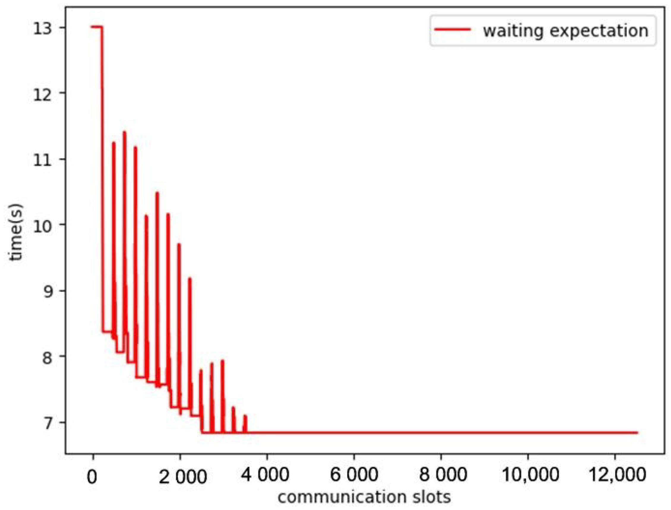
Thus, we define the concept of expected wait as a metric; it is the average time the slots need to wait before sending a message packet, with the requirement of sending the message packet appearing at a random time. It is defined as:

$$t_{exp}=\frac{t_{slot}}{N}\sum _{i=1}^N{n}_{slotsWait}^i$$

where $t_{slot}$ is the length of a slot, and N is the number of nodes in the network and also the length of the frame; $n_{slotsWait}^i$ means the number of slots between slot i and the next slot occupied by the current node.

5.2. Core Algorithm for Forwarding Guide

The forwarding guide can be described with Algorithm 4. The output of the algorithm is the content that will be packed into the communication packet sent by the current slot as:

$$(i{d}_{self},c_{self},i{d}_{next},S_{msg})$$

The inputs of the algorithm include communication table $L_f$, which is provided by the slot distributor, and the key content contained in the message packet received as 

$$(i{d}_{self}^{sender},c_{self}^{sender},i{d}_{next}^{sender},S_{msg}^{sender})$$

We initialize the algorithm in Line 1 and 2, where we define a set $S_{1\text{-}neighbor}$ to save the IDs of the current node’s first-order neighbors, and $S_{cost}=\left\{c_i\right|i_{1\text{-}neighbors}\}$ to save the costs for each neighbor to send a message to the base station. Initially, the two sets are all empty. Then, the while loop in Lines 3–27 defines the current node’s behavior in relation to relaying messages in each slot. Basically, the behavior is composed of three parts, where Line 4 and Lines 12–14 maintain the neighbors, Lines 5–9 and Lines 15–17 deal with the message content to be sent, and Lines 18–24 search for the best path to relay the message packet.

At the beginning of a new slot in Line 3, the current node deletes the lost neighbor. As in Section 4, one node should speak at least once during a frame, so if a neighbor fails to speak for a whole frame, it is lost and will be deleted. Then, the current node checks if it should speak in Line 5 and then broadcasts a message packet containing self ID $i{d}_{self}$, the current cost to relay the message packet $c_{self}$, its successor node to relay the message packet $i{d}_{next}$, and all data needing to be sent $S_{msg}$. If $i{d}_{next}=-1$, the current node has not established a path to the base station, and no successor exists and $S_{msg}$ cannot be relayed. Therefore, the node will clear its storage. Otherwise, $S_{msg}$ will be handed over to another node, so $S_{msg}$ will be set empty.

On receiving a message in Line 11, the node updates the information about its neighbor by either adding new information or by replacing old information with new information, as in Lines 13–14. If the current node is the successor of the sender, then $S_{msg}^{sender}$ is stored and awaiting being forwarded, as in Lines 15–17. Then, in Lines 18–24, the current node tries to update its successor, finding a better way to relay the message. This is achieved by setting the first-order neighbor with the lowest total cost as the current successor. It is proved in Section 5.3 that the path will converge to the shortest path.

Algorithm 4 Forwarding Guide

Input: Communication table $L_f$, $(i{d}_{self}^{sender},c_{self}^{sender},i{d}_{next}^{sender},S_{msg}^{sender})$ contained in communication packet received

Output: $(i{d}_{self},c_{self},i{d}_{next},S_{msg})$, as information that should be contained in the message packet to send

1: $S_{1\text{-}neighbor}\leftarrow \varphi ,S_{cost}\leftarrow \varphi$ 2: $i{d}_{next}=-1$, $S_{msg}\leftarrow \varphi$,$c_{self}\leftarrow 0$ if current node is base station and $c_{self}\leftarrow \infty$ otherwise 3: while New slot with address=$i{d}_{slot}$ do 4:     Update $S_{1\text{-}neighbor}$ and $S_{cost}$ by deleting neighbors that fail to speak for a whole frame 5:     if $L_f\left(i{d}_{slot}\right)$=1 then 6:         Send message packet containing $(i{d}_{self},c_{self},i{d}_{next},S_{msg})$ 7:         if $i{d}_{next}\ne -1$ then 8:            $S_{msg}\leftarrow \varphi$ 9:         end if 10:     else 11:         if receive message packet successfully then 12:             message packet contains $(i{d}_{self}^{sender},c_{self}^{sender},i{d}_{next}^{sender},S_{msg}^{sender})$ 13:            $S_{1\text{-}neighbor}\leftarrow S_{1\text{-}neighbor}\cup i{d}_{self}^{sender}$ 14:            Update $S_{cost}$ with $c_{self}^{sender}$ 15:            if $i{d}_{next}^{sender}=i{d}_{self}$ then 16:                $S_{msg}\leftarrow S_{msg}\cup S_{msg}^{sender}$ 17:            end if 18:            Calculate expected wait with $$t_{exp}\leftarrow \frac{t_{slot}}{N}\sum _{i=1}^N{n}_{slotsWait}^i$$ 19:            for $i\in S_{1\text{-}neighbor}$ do 20:                $t_{cost}^i\leftarrow t_{exp}+c\left(i\right),c\left(i\right)\in S_{cost}$ 21:                if $t_{cost}^i<c_{self}$ then 22:                    $c_{self}\leftarrow t_{cost}^i$,$i{d}_{next}\leftarrow i$ 23:                end if 24:            end for 25:         end if 26:     end if 27: end while

5.3. Convergence of the Algorithm

In this section, we explain the convergence of the algorithm. This can be proved with the help of Dijkstra’s algorithm. We model the sensor network as a directed graph model, with nodes being vertexes, composing set V. For edges, to satisfy the definition of the classic Dijkstra Algorithm, for a pair of first-order neighbors, an edge is assigned from the receiver pointing at the sender, with the weight of this edge being the expected wait of the sender. Thus, we obtain the edge set E and the weight set W. Based on this definition, we write the classic Dijkstra Algorithm as Algorithm 5, where $dist[s,t]$ indicates the total cost for node s to receive a message packet from node t. Set S stores the vertexes that already find their shortest path to the source vertex s, where vertex s indicates the base station that collects all messages in the sensor network. The weight $w_{s,t}$ is the expected wait of t if s is its first-order neighbor. If $t=s$, $w_{s,t}=0$. If $t\ne s$ and s is not a first-order neighbor of t, then $w_{s,t}=\infty$.

Following the definitions above, we abstract the part of searching for the forwarding path in Algorithm 4 as Algorithm 6.

Algorithm 5 Dijkstra Algorithm

Input: Directed graph $G=(V,E,W)$ with weight

Output: All the shortest paths from source vertex s to every other vertex

1: $S\leftarrow s$ 2: $dist[s,s]\leftarrow 0$ 3: for $v_i\in V-s$ do 4:     $dist[s,v_i]\leftarrow w(s,v_i)$ (when $v_i$ not found, $dist[s,v_i]\leftarrow \infty$) 5: end for 6: while $V-S\ne \varphi$ do 7:     find $mi{n}_{v_j\in V}dist[s,v_i]$ from the set $V-S$ 8:     $S\leftarrow S\cup v_j$ 9:     for $v_i\in V-S$ do 10:         if $dist[s,v_j]+w_{j,i}<dist[s,v_i]$ then 11:             $dist[s,v_i]\leftarrow dist[s,v_j]+w_{j,i}$ 12:         end if 13:     end for 14: end while

Algorithm 6 Abstraction of Algorithm 4

1: while True do 2:     for $v\in V$ do 3:         for $v_j\in S_{1\text{-}neighbor}\left(v\right)$ do 4:            if $dist[s,v_j]+w_{j,i}<dist[s,v_i]$ then 5:                $dist[s,v_i]\leftarrow dist[s,v_j]+w_{j,i}$ 6:            end if 7:         end for 8:     end for 9: end while

By comparing Algorithm 5 with Algorithm 7, we can see that both algorithms set the same initial conditions. Lines 5–7 in the Dijkstra Algorithm are used to set a termination condition, while Algorithm 7 does not. However, as the sensor network keeps working, it can be treated that the algorithm will loop forever, exceeding the time needed for convergence, and thus a termination condition is unnecessary. Then, in Algorithm 7, $dist[s,v_i]$ will not change when $v_i\notin V-S$b because the node cannot find a shorter path; the same thing happens in the Dijkstra Algorithm. In the Dijkstra Algorithm, we update $dist[s,v_i]$ with $v_j$, which is currently not in S while having the shortest path to s, as in Lines 9–13. Even though $dist[s,v_i]$ may change in Lines 5–10, it will finally be updated in Lines 11–15, following the same operation in the Dijkstra Algorithm. Thus, the two algorithms are equivalent at this stage, except that for Dijkstra’s Algorithm, nodes need to know the whole graph, while our algorithm can work only based on local information. As a result, with the forwarding guide, the sensor network can finally converge to the state where message packets can be relayed to the base station with the shortest expected wait.

Algorithm 7 Another form of Algorithm 6

1: while True do 2:     for $v_i\in V$ do 3:         if $v_i\in V-S$ then 4:            for $v_j\in S_{1\text{-}neighbor}\left(v\right)$ do 5:                if $v_j\in S$ then 6:                    Nothing will happen 7:                end if 8:                if $v_j\in V-S\wedge dist[s,v_j]\ne mi{n}_{v_i\in V-S}dist[s,v_i]$ then 9:                    $dist[s,v_i]$ may be updated, but cannot ensure reaching the minimum value 10:                end if 11:                if $v_j\in V-S\wedge dist[s,v_j]=mi{n}_{v_i\in V-S}dist[s,v_i]$ then 12:                    if $dist[s,v_j]+w_{j,i}<dist[s,v_i]$ then 13:                        $dist[s,v_i]\leftarrow dist[s,v_j]+w_{j,i}$ 14:                    end if 15:                end if 16:            end for 17:         else 18:            Nothing will happen 19:         end if 20:     end for 21: end while

6. Experiment

In this section, we evaluate the effectiveness of our method with simulation experiments. Two sets of experiments are carried out. We first check the performance of the slot distributor, showing that it can converge to the state where no collisions exist in the network. Then, the performance of the forwarding guide is checked by comparing it with that of the Aloha protocol.

6.1. Performance of the Slot Distributor

We first check the performance of the slot distributor. Two sets of experiments are carried out. In the first experiment, we exhibit the performance of a relatively small network in detail, showing readers how the coordinator works. In the network, 25 nodes are deployed as a grid formation, with the edge length of 200 m. The communication range is set to 300 m, satisfying the situation of high-frequency acoustic communication devices. The deployment is shown in Figure 7.

The performance of the method is shown in Figure 8, which shows the communication results in each frame with the number of successes and failures shown. The pulse in the figure indicates nodes trying to occupy slots, which may introduce collisions into the network. However, as time goes on, most nodes have already occupied optimum slots, and the deployment of pheromone clues prohibits nodes from occupying more slots. Finally, the network converges to the state without communication collision.

Figure 9 shows the average occupation of slots by nodes. The available slots are those slots not occupied by a first-order or second-order neighbor, and the occupied slots are those slots actually occupied by nodes. From this figure, we can see that nodes are trying to occupy more available slots, and finally, almost all valid slots are occupied by nodes in the network.

As a result, from Figure 10, we notice that the average expected wait keeps dropping and finally converges to a relatively small value. In Figure 11, we show the final slots occupied by a sub-network consisting of Node 19 and its neighbors. We see that Node 19 has does not have all of its slots occupied by either its first-order neighbors or by its second-order neighbors. There are no slots occupied by more than one of its first-order neighbors, so collision will not occur among the first-order neighbors. In some cases, a slot is occupied by a first-order neighbor or more than one second-order neighbor. For example, Slot 7 is occupied by Node 7 (i.e., a second-order neighbor of Node 19) and Node 24 (i.e., a first-order neighbor of Node 19) at the same time. This is reasonable because Node 7 and Node 24 are neither first-order neighbors nor second-order neighbors, and this will not cause communication collision.

To verify that our method still works on large networks, we test a network containing 100 nodes, with nodes deployed randomly in the area of interest, as displayed in Figure 12. The communication result in each frame along time is shown in Figure 13. Apparently, the network still converges and our method works.

In the communication packet, $(i{d}_{self},S_{neighbor},S_{abandon})$ are the data used to coordinate slot distribution. For a sensor network containing fewer than 256 nodes, the ID of a node can be encoded as one byte; thus, the maximum value is $1+2N$ bytes. In a method similar to the one proposed in [4], the data used to coordinate slot distribution contain

$$(i{d}_{self},S_{1\text{-}neighbor},S_{2\text{-}neighbor},Slo{t}_{1\text{-}neighbor},Slo{t}_{2\text{-}neighbor}),$$

with $S_{1\text{-}neighbor}$ all first-order neighbors, $Slo{t}_{1\text{-}neighbor}$ the slot occupied by each first-order neighbor, $S_{2\text{-}neighbor}$ all the second-order neighbors, and $Slo{t}_{2\text{-}neighbor}$ slots occupied by each second-order neighbor. Thus, in the worst case, the data for coordination reach $1+N^2$ bytes, much larger than our proposed method. Consequently, the method in [4] can only be used in radio communication, while our method satisfies the requirements of underwater acoustic communication.

6.2. Testing the Forwarding Guide

We then test the performance of the forwarding guide and compare its performance with that of the classic Aloha protocol. The distribution of slots is as in Section 6.1. Assume Node 24 detects a target at a random time and needs to report this message to node 0, i.e., the base station. Without losing generality, during transmission of the message, other nodes will not keep silent because they need to exchange information, such as sending a message packet to check the connectivity of the network or message packets generated by other nodes.

We compare the performance of our forwarding guide with that of the classic Aloha protocol. For our forwarding guide, the communication table is the one generated in Section 6.1. According to the analysis of the slot distributor, the communication table finally generated features each node occupying at least one slot. Thus, the exchanging of information by other nodes will not bother the transmission of the message packet from Node 24. However, for the classic Aloha protocol, if other nodes do not need to exchange information, they can keep silent. As we assume nodes always need to exchange information, we set each node with the same probability of broadcasting a message. As the time for message propagation is related to the probability of a node sending a message packet at a slot, we test the situation with sending probability $p=0.1,0.2,0.3,0.4$. For each setting, we repeat the experiment 20 times. The result is shown in Figure 14.

In Figure 14, we measure the time needed to send the message packet from Node 24 to Node 0 with the number of slots. We highlight the performance of our forwarding guide in red, while that of the classic Aloha protocol is in blue. It is shown that it takes 30 slots on average to relay a message packet from the node farthest from the base station to its destination. However, for the Aloha protocol, it takes at least 40 slots for the message packet to reach its destination, around 30% longer than that of our forwarding guide. Further, the variation of our forwarding guide is smaller than that of the Aloha protocol with different sending probabilities, indicating that our forwarding guide performs not only better but also more steadily. Additionally, with the increase of p, the time spent by the Aloha protocol shows a tendency to first decrease and then increase. This is because when the p is small, the probability of a node speaking is too small, such that a node needs to wait a long time before sending a message. When the p is big, the chance of communication collision increases, extending the time for the message to reach its destination successfully in return. This implies that with the Aloha protocol, the sending probability needs to be set carefully to get the best performance. Meanwhile, our forwarding guide has no parameters that need to be adjusted, making it easier to be adopted in an application.

7. Conclusions

In this paper, we propose a method to coordinate message transmission in a large-scale wireless underwater sensor network. The coordinator consists of a slot distributor, which provides each node with the slots it should occupy, and a forwarding guide, which indicates the next node to relay the message packet. As a result, with the communication coordinator, the communication process can be coordinated in a self-organized way, and it fits for networks consisting of a large number of randomly deployed nodes. The network can converge to the state without communication collision, and the coordinate information will not use many communication resources, which fits for underwater acoustic communication. The message can be transmitted to the base station following the shortest path defined with expected waits, outperforming the Aloha protocol.

The main shortcoming of the current method is that we are using a fixed-length TDMA framework. Thus, the frame length will grow with the addition of nodes to the network. This problem can be solved with a dynamic-length TDMA framework, and that is what we are working on at present.

References

1. Cao, M.; Bie, H.; Hu, X. Behavior Composition for Marine Pollution Source Localization Using a Mobile Sensor Network. Appl. Sci. 2022, 12, 5767. [Google Scholar] [CrossRef]
2. Lončar, I.; Babić, A.; Arbanas, B.; Vasiljević, G.; Petrović, T.; Bogdan, S.; Mišković, N. A Heterogeneous Robotic Swarm for Long-Term Monitoring of Marine Environments. Appl. Sci. 2019, 9, 1388. [Google Scholar] [CrossRef] [Green Version]
3. Cho, A.R.; Yun, C.; Lim, Y.K.; Choi, Y. Asymmetric Propagation Delay-Aware TDMA MAC Protocol for Mobile Underwater Acoustic Sensor Networks. Appl. Sci. 2018, 8, 962. [Google Scholar] [CrossRef] [Green Version]
4. Cao, Y.; Chen, C.; St-Onge, D.; Beltrame, G. Distributed TDMA for Mobile UWB Network Localization. IEEE Internet Things J. 2021, 8, 13449–13464. [Google Scholar] [CrossRef]
5. Tarafder, P.; Choi, W. MAC Protocols for mmWave Communication: A Comparative Survey. Sensors 2022, 22, 3853. [Google Scholar] [CrossRef]
6. Gussen, C.M.; Diniz, P.S.; Campos, M.L.; Martins, W.A.; Costa, F.M.; Gois, J.N. A survey of underwater wireless communication technologies. J. Commun. Inf. Syst. 2016, 31, 242–255. [Google Scholar] [CrossRef]
7. Akyildiz, I.F.; Pompili, D.; Melodia, T. Underwater acoustic sensor networks: Research challenges. Ad Hoc Netw. 2005, 3, 257–279. [Google Scholar] [CrossRef]
8. Melodia, T.; Kulhandjian, H.; Kuo, L.C.; Demirors, E. Advances in underwater acoustic networking. Mob. Ad Hoc Netw. Cut. Edge Dir. 2013, 804–852. [Google Scholar] [CrossRef]
9. Lanzagorta, M. Underwater Communications; Synthesis Lectures on Communications Series; Morgan & Claypool Publishers: San Rafael, CA, USA, 2012; Volume 5, pp. 1–129. [Google Scholar]
10. Che, X.; Wells, I.; Dickers, G.; Kear, P.; Gong, X. Re-evaluation of RF electromagnetic communication in underwater sensor networks. IEEE Commun. Mag. 2010, 48, 143–151. [Google Scholar] [CrossRef]
11. Sexton, D. Subsea Communications, RPSEA Final Report; GE Global Research: New York, NY, USA, 2011. [Google Scholar]
12. VK5BR, L.B. Underwater Radio Communication; Amateur Radio, 1987. [Google Scholar]
13. Palmeiro, A.; Martin, M.; Crowther, I.; Rhodes, M. Underwater radio frequency communications. In Proceedings of the IEEE OCEANS 2011 IEEE-Spain, Santander, Spain, 6–9 June 2011; pp. 1–8. [Google Scholar]
14. Hanson, F.; Radic, S. High bandwidth underwater optical communication. Appl. Opt. 2008, 47, 277–283. [Google Scholar] [CrossRef]
15. Doniec, M.; Vasilescu, I.; Chitre, M.; Detweiler, C.; Hoffmann-Kuhnt, M.; Rus, D. AquaOptical: A lightweight device for high-rate long-range underwater point-to-point communication. In Proceedings of the IEEE OCEANS 2009, Bremen, Germany, 11–14 May 2009; pp. 1–6. [Google Scholar]
16. Anguita, D.; Brizzolara, D.; Parodi, G.; Merrett, G.; Tan, Y. Prospects and problems of optical diffuse wireless communication for underwater wireless sensor networks (UWSNs). Wireless Sensor Networks: Application-Centric Design; InTech: Rijeka, Croatia, 2010; pp. 275–300. [Google Scholar]
17. Zhang, H.; Dong, Y. Link misalignment for underwater wireless optical communications. In Proceedings of the IEEE 2015 Advances in Wireless and Optical Communications (RTUWO), Riga, Latvia, 5–6 November 2015; pp. 215–218. [Google Scholar]
18. Gabriel, C.; Khalighi, M.A.; Bourennane, S.; Léon, P.; Rigaud, V. Monte-Carlo-based channel characterization for underwater optical communication systems. J. Opt. Commun. Netw. 2013, 5, 1–12. [Google Scholar] [CrossRef] [Green Version]
19. Stojanovic, M.; Catipovic, J.; Proakis, J.G. Adaptive multichannel combining and equalization for underwater acoustic communications. J. Acoust. Soc. Am. 1993, 94, 1621–1631. [Google Scholar] [CrossRef]
20. Jensen, F.B.; Kuperman, W.A.; Porter, M.B.; Schmidt, H.; Tolstoy, A. Computational Ocean Acoustics; Springer Science & Business Media: New York, NY, USA, 2011; Volume 794. [Google Scholar]
21. Preisig, J. Acoustic propagation considerations for underwater acoustic communications network development. ACM SIGMOBILE Mob. Comput. Commun. Rev. 2007, 11, 2–10. [Google Scholar] [CrossRef]
22. Li, B.; Zhou, S.; Huang, J.; Willett, P. Scalable OFDM design for underwater acoustic communications. In Proceedings of the 2008 IEEE International Conference on Acoustics, Speech and Signal Processing, Las Vegas, NV, USA, 31 March–4 April 2008; pp. 5304–5307. [Google Scholar]
23. Alfouzan, F.A. Energy-Efficient Collision Avoidance MAC Protocols for Underwater Sensor Networks: Survey and Challenges. J. Mar. Sci. Eng. 2021, 9, 741. [Google Scholar] [CrossRef]
24. Wang, X.; Kong, L.; Kong, F.; Qiu, F.; Xia, M.; Arnon, S.; Chen, G. Millimeter wave communication: A comprehensive survey. IEEE Commun. Surv. Tutor. 2018, 20, 1616–1653. [Google Scholar] [CrossRef]
25. Zhang, W.; Wang, X.; Han, G.; Peng, Y.; Guizani, M.; Sun, J. A load-adaptive fair access protocol for MAC in underwater acoustic sensor networks. J. Netw. Comput. Appl. 2021, 173, 102867. [Google Scholar] [CrossRef]
26. Han, G.; Long, X.; Zhu, C.; Guizani, M.; Zhang, W. A High-Availability Data Collection Scheme based on Multi-AUVs for Underwater Sensor Networks. IEEE Trans. Mob. Comput. 2020, 19, 1010–1022. [Google Scholar] [CrossRef]
27. Wang, C.; Shen, X.; Wang, H.; Mei, H. Energy-efficient collection scheme based on compressive sensing in underwater wireless sensor networks for environment monitoring over fading channels. Digit. Signal Process. 2022, 127, 103530. [Google Scholar] [CrossRef]
28. Khan, Z.U.; Gang, Q.; Muhammad, A.; Muzzammil, M.; Khan, S.U.; Affendi, M.E.; Ali, G.; Ullah, I.; Khan, J. A comprehensive survey of energy-efficient MAC and routing protocols for underwater wireless sensor networks. Electronics 2022, 11, 3015. [Google Scholar] [CrossRef]
29. Yunus, F.; Ariffin, S.H.; Zahedi, Y. A survey of existing medium access control (MAC) for underwater wireless sensor network (UWSN). In Proceedings of the IEEE 2010 Fourth Asia International Conference on Mathematical/Analytical Modelling and Computer Simulation, Kota Kinabalu, Malaysia, 26–28 May 2010; pp. 544–549. [Google Scholar]
30. Akyildiz, I.F.; Pompili, D.; Melodia, T. Challenges for efficient communication in underwater acoustic sensor networks. ACM Sigbed Rev. 2004, 1, 3–8. [Google Scholar] [CrossRef] [Green Version]
31. Sozer, E.; Stojanovic, M.; Proakis, J. Underwater acoustic networks. IEEE J. Ocean. Eng. 2000, 25, 72–83. [Google Scholar] [CrossRef]
32. Wei, X.; Guo, H.; Wang, X.; Wang, X.; Wang, C.; Guizani, M.; Du, X. A Co-Design-Based Reliable Low-Latency and Energy-Efficient Transmission Protocol for UWSNs. Sensors 2020, 20, 6370. [Google Scholar] [CrossRef]
33. Valerio, V.D.; Petrioli, C.; Pescosolido, L.; Van Der Shaar, M. A reinforcement learning-based data-link protocol for underwater acoustic communications. In Proceedings of the 10th International Conference on Underwater Networks & Systems, Arlington, VA, USA, 22–24 October 2015; pp. 1–5. [Google Scholar]
34. Wang, H.; Wang, S.; Bu, R.; Zhang, E. A novel cross-layer routing protocol based on network coding for underwater sensor networks. Sensors 2017, 17, 1821. [Google Scholar] [CrossRef] [Green Version]
Figure 1. Illustration of a wireless underwater sensor network. Nodes are randomly deployed and float at a certain depth. The nodes communicate with each other via underwater acoustic communication. There is a special node called a base station that is connected with a radio antenna floating at the surface of the water. Information obtained by sensor nodes is sent to the base station, and the base station sends messages to the control center via radio. As communication collision can happen if acoustic signals are sent improperly, each node is equipped with a controller called a communication coordinator, which is used to control when and what a node broadcasts via acoustic signals. The communication coordinator is designed in this paper.
Applsci 13 04330 g001
Figure 2. Illustration of neighbors of Node A. Dots in the figure denote sensor nodes, and the ring with the same color as a node indicates the communication range of the node. Nodes B, D, and E are the first-order neighbors of Node A because they are within the communication range of Node A. Node C is the second-order neighbor of A because it is the first-order neighbor of B while not a first-order neighbor of A.
Applsci 13 04330 g002
Figure 3. The two situations that can cause communication collisions. Dots denote sensor nodes, and the concentric circles with the same color indicate the node is broadcasting a message. A node with a check mark indicates it has received a message successfully, while a cross indicates it has failed to receive a message. Subfigure (a) exhibits communication collisions between a pair of first-order neighbors. Nodes A and B are a pair of first-order neighbors, and they are speaking simultaneously. In this situation, Nodes A and B fail to receive messages, while Nodes C and E receive messages successfully. Subfigure (b) exhibits communication collisions between a pair of second-order neighbors. Nodes A and C are a pair of second-order neighbors that are speaking simultaneously. Node B is the first-order neighbor of both A and B. Node B receives both signals at the same time, so it is unable to parse messages in either of the signals.
Applsci 13 04330 g003
Figure 4. TDMA framework. Time is divided into a sequence of frames, with each frame further scattered into a set of slots.
Applsci 13 04330 g004
Figure 5. Calculation of preference.
Applsci 13 04330 g005
Figure 6. Example of communication lock. For the mini network consisting of 4 nodes, if Node 0 and Node 1 occupy the same slots while Node 2 and Node 3 occupy the same slots, they are trapped in a communication lock. Nodes that occupy the same slots are marked with the same color.
Applsci 13 04330 g006
Figure 7. Node distribution in a sensor network consisting of 25 nodes. Dots denote sensor nodes, and the number beside indicates the ID of the sensor node. The ring around a dot is the communication range of the node. The edge of each grid is 200 m, and the communication range for each node is 300 m.
Applsci 13 04330 g007
Figure 8. Communication results in each frame. “sent messages” denotes the total number of message packets sent by sensor nodes in the whole network in a frame. “successful messages” indicates message packets successfully received by all nodes within the communication range, and “failed messages” indicates message packets not successfully received by all nodes within the communication range because of communication collisions. Note that there is a case where a message packet is received successfully by some neighbors, while a collision happens with other neighbors; we treat this message packet as failed to be sent.
Applsci 13 04330 g008
Figure 9. The average number of slots occupied by nodes over time. For each node, its available slots denote the communication slots not occupied by any of the node’s first-order or second-order neighbors. The average available slots represent the average number of all nodes’ available slots, and the average occupied slots denote the average number of available slots occupied by nodes.
Applsci 13 04330 g009
Figure 10. The average expected wait over time, i.e., the average value of expected wait of all nodes in the sensor network in each slot.
Applsci 13 04330 g010
Figure 11. The final situation of slots occupied in the sub-network centered by Node 19. The horizontal direction denotes the IDs of slots, while the vertical direction indicates the IDs of nodes. The red dots represent slots occupied by Node 19. The blue dots indicate slots occupied by first-order neighbors of Node 19, and the green dots second-order neighbors. From the red line, it is obvious that the slots occupied by Node 19 are not occupied by any of its first- or second-order neighbors, and thus communication collisions will not occur when Node 19 speaks. Meanwhile, all slots have already been occupied by at least one node, indicating that Node 19 has already occupied all available slots.
Applsci 13 04330 g011
Figure 12. A sensor network with 100 randomly deployed nodes. The dots with the numbers beside them are nodes and their IDs. The nodes can be deployed randomly with the only requirement that they can form a connected graph. The distribution is generated by randomly picking a node already deployed and placing a new node randomly within its communication range, repeating this process until the number of nodes deployed reaches the target size.
Applsci 13 04330 g012
Figure 13. Communication result in each frame for network consisting of 100 nodes.
Applsci 13 04330 g013
Figure 14. Time comparison to send a message packet to the base station with the proposed method and the classic Aloha protocol using different speaking probabilities p.
Applsci 13 04330 g014