Assessment of the Critical Defect in Additive Manufacturing Components through Machine Learning Algorithms

Abstract

The design against fatigue failures of Additively Manufactured (AM) components is a fundamental research topic for industries and universities. The fatigue response of AM parts is driven by manufacturing defects, which contribute to the experimental scatter and are strongly dependent on the process parameters, making the design process rather complex. The most effective design procedure would involve the assessment of the defect population and the defect size distribution directly from the process parameters. However, the number of process parameters is wide and the assessment of a direct relationship between them and the defect population would require an unfeasible number of expensive experimental tests. These multivariate problems can be effectively managed by Machine Learning (ML) algorithms. In this paper, two ML algorithms for assessing the most critical defect in parts produced by means of the Selective Laser Melting (SLM) process are developed. The probability of a defect with a specific size and the location and scale parameters of the statistical distribution of the defect size, assumed to follow a Largest Extreme Value Distribution, are estimated directly from the SLM process parameters. Both approaches have been validated using literature data obtained by testing the AlSi10Mg and the Ti6Al4V alloy, proving their effectiveness and predicting capability.

1. Introduction

The assessment of the fatigue response of components produced through Additive Manufacturing (AM) processes is a challenging topic for researchers. The main issue is that manufacturing defects (e.g., lack of fusion and porosities) drive the fatigue response of AM parts, typically characterized by a large experimental scatter and lower strength compared to that of traditionally built parts [1,2,3]. Defining reliable fatigue design methodologies is mandatory to extend the use of AM components even in critical structural applications and to further boost their diffusion.

According to the literature, the size of manufacturing defects is the main factor affecting the fatigue response [4,5,6]. For defects with irregular morphology, typical of AM parts, an equivalent size can be considered, e.g., following the rules reported in [4,5] and based on the fracture mechanics approach. Given the defect size, different damage-tolerant methodologies can be reliably employed [4,7,8,9] to design components. However, the main challenge for a safe design is predicting the most critical defect that will appear in the component during manufacturing. For example, micro-CT inspections provide the population of defects, but this approach is not effective since it can only be applied after having produced the part, whose safety against fatigue loads should have been already verified in the design stage. Alternatively, the critical defect in the component volume can be predicted if the defect distribution is available or has been estimated from fatigue tests and following analyses of the fracture surfaces. This approach is effective only if the part will be produced with the same process parameters, since the defect population is strongly dependent on them [6,10,11]. The correlation between the process parameters and the defect population should therefore be assessed. However, the number of process parameters for manufacturing AM parts is large, e.g., at least five for the Selective Laser Melting (SLM) process, one of the most used AM techniques. Accordingly, a correlation and, above all, the interactions between different process parameters and the critical defect cannot be experimentally detected, since an unfeasible number of experimental tests would be required. On the other hand, this multivariate problem concerning the fatigue response of AM parts can be effectively managed with Machine Learning (ML) algorithms. In the literature, ML algorithms have been increasingly used for dealing with the defect population and, in general, the fatigue response of AM components. For example, in [12], an ML methodology trained on artificial data is exploited to assess the fatigue limit of AM Ti6Al4V and SS316L alloys. The influence of process parameters is embedded in the computational approach used to generate data. In [13], the efficiency of both shallow and deep neural networks in predicting the effect of thermal and shot peening post-treatment on the fatigue life of AM AlSi10Mg parts is investigated. The models are trained on the experimental data of notched specimens produced with a specific set of printing parameters. In [14], a probabilistic physics-guided model for the prediction of the stress–life relationship of SLM Ti6Al4V starting from process parameters is defined, with soft constraints on the S-N curve trend imposed and without accounting for the defect influence. In [15], an Artificial Neural Network (ANN) is developed to assess the lowest stress to be used for the design of AM components starting from the material hardness and the defect size. In [16], a Physics-Informed ML algorithm is developed for the prediction of the fatigue life of AM components. Phenomenological constraints based on Linear Elastic Fracture Mechanics are embedded in the developed algorithm, making it appropriate even when the dataset for training is limited. Moreover, prediction bands in place of deterministic predictions are effectively considered to account for all the source uncertainty typical of the AM fatigue response. In [17], a reinforcement ML algorithm is developed to assess the posterior distribution of the fatigue strength of an AM AlSi12 alloy. The Bayesian inferential statistics and the Metropolis Monte Carlo algorithms are used. The model has been validated on AlSi12 alloy results obtained through tests up to the Very High Cycle Fatigue (VHCF) life region. In [18], the fatigue life of AM AlSi10Mg specimens is predicted by using Continuous-Damage-Mechanics (CDM)-informed ML algorithms. In [19], the fatigue life of AM components is predicted starting from the process parameters with an NN algorithm and a Physics-Informed NN algorithm based on the Murakami theory [4], to model the influence of defect size and microstructure. The developed ML algorithms have been validated on AlSi10Mg literature experimental datasets. In [20], Artificial Neural Network (ANN), Support Vector Machine (SVR) and Random Forest (RF) models are employed to investigate the influence of defects on the High Cycle Fatigue (HCF)-VHCF response of AM AlSi10Mg specimens. Moreover, these algorithms have been used to predict the VHCF life from the layer thickness process parameter, the stress ratio and the defect properties. In [21], the fatigue life of an industrial AM Ti6Al4V demonstrator is predicted with a simulation-based approach and by employing a supervised Machine Learning algorithm. According to this literature review, ML algorithms can be reliably employed for the assessment of the fatigue response of AM components, with promising results. Approaches based on ML algorithms allow for simplifying the design against fatigue failures of AM components by exploiting already-available literature data and by embedding physical and phenomenological models, if the data for the training process are limited.

In this paper, ML algorithms are employed to estimate the most critical defect in a part to be produced by SLM. The process parameters and the component volume are considered as the input of the developed Neural Network (NN) architecture. By also considering the component volume as an NN input, the dependence between the defect size and the part volume is also accounted for, i.e., the size effect is reliably modelled. The influence of surface roughness has not been accounted for, even if it is widely known that it significantly affects the fatigue response of AM parts and is among the most detrimental factors [5]. However, the surface roughness can be controlled through appropriate surface treatments. On the other hand, the focus of the present work is to estimate rare and large defects that randomly form in parts produced with optimized process parameters and contribute to lower the fatigue response of AM parts even if characterized by the same roughness of traditionally built parts.

Two approaches are followed for designing the NN architectures: the first one provides the probability of a defect with a specific size for a set of process parameters and the part volume. The second one provides the location and the scale parameters of the statistical distribution of the defect size, assumed to follow a Largest Extreme Value Distribution (LEVD) for a set of process parameters and the part volume. Both approaches have been validated on literature data obtained by testing the AlSi10Mg and the Ti6Al4V alloy.

It must be noted that several works proposing ML algorithms for the structural integrity of components have been proposed in the last years, but those focusing on the fatigue response of AM components are the ones previously analyzed, to the authors’ best knowledge. However, none of these models aims at predicting the defect size starting from the process parameters. Indeed, the defect population is strongly dependent on the process parameters and the most effective damage-tolerant fatigue design should start from the process parameters. This idea and its implementation through the developed ML algorithms open the path to an innovative way of designing AM components.

2. Machine Learning and Defect Size: Algorithms

In this Section, the Machine Learning algorithms developed to predict the defect size are described in detail. Section 2.1 focuses on defects typical of AM components and on their statistical distribution. In Section 2.2, details on the ML input data and the characteristics of the training dataset are provided. In Section 2.3, the ML algorithms developed to assess the probability of a specific defect size (Section 2.3.1) and the location and the scale parameters of the LEVD followed by the defect size random variable (Section 2.3.2) are described. Finally, Section 2.4 focuses on the procedure followed to validate the ML algorithms, i.e., the k-fold cross-validation scheme.

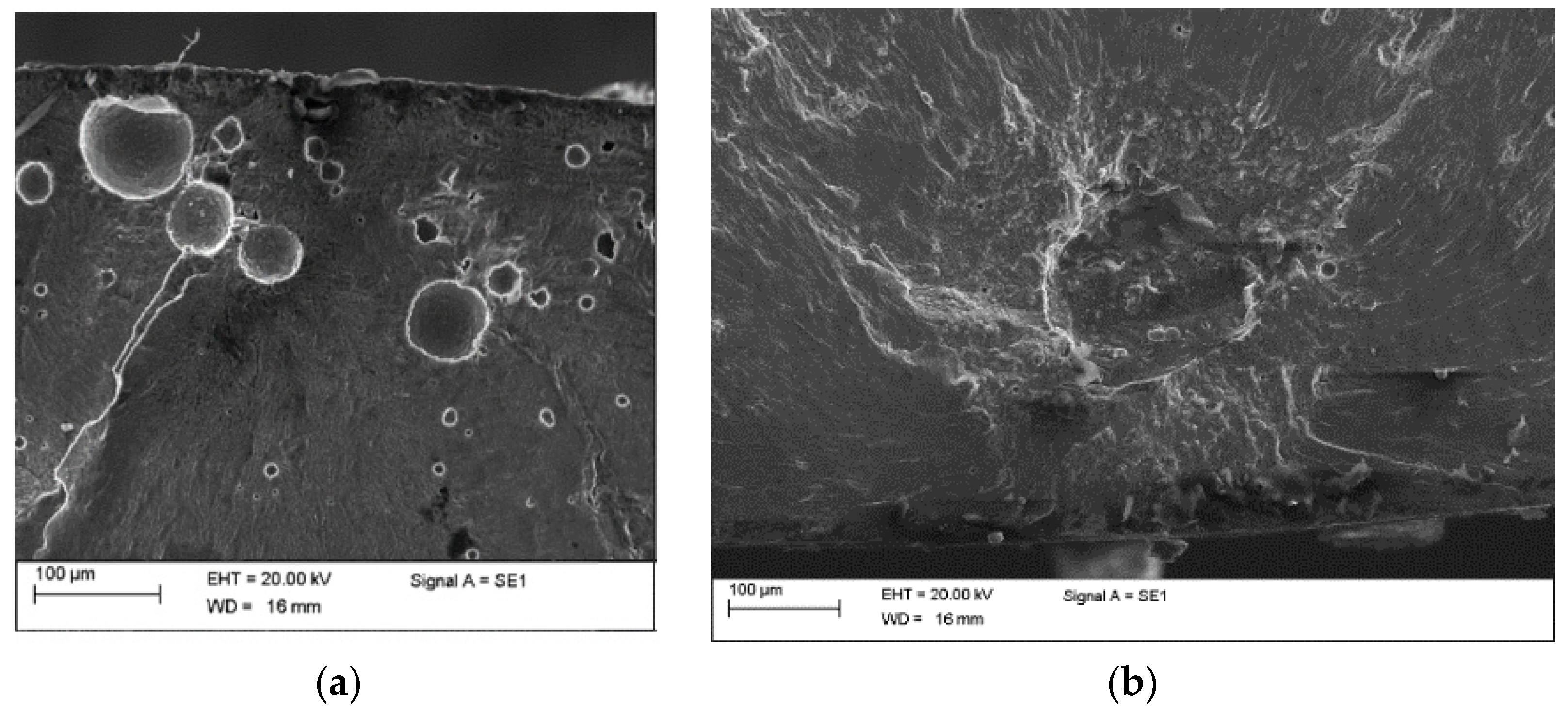
2.1. Defects in AM Components

The main reason for the lower fatigue response of AM parts, if compared to that of traditionally built components, is the formation of large manufacturing defects during the AM process. Defects are well-known to significantly affect the fatigue response, since they act as stress concentrators and enhance the crack nucleation process. For this reason, a damage-tolerant approach should be employed when AM components are to be designed, with the influence of defects that cannot be neglected to ensure a safe design. Figure 1 shows the most common AM defects, pores (Figure 1a) and lack of fusion defects (Figure 1b).

In order to properly apply the damage-tolerant approaches developed in the literature, the defect size in the component should be known or reliably predicted. According to [4], the defect size, rather than the defect type or morphology, mainly affects the fatigue response. In particular, the area of the defect projected in a direction perpendicular to the maximum applied stress can be considered as the characteristic defect size, $\sqrt{a_c}$, and for the analysis of the fatigue response. It is of utmost importance, therefore, to properly measure or predict the $\sqrt{a_c}$ parameter in components. Moreover, according to [4], an equivalent defect size can be estimated for defects with complex shapes, by considering the fracture mechanics approach. In the following, therefore, the $\sqrt{a_c}$ parameter is considered as the characteristic defect size and will be employed for the developed ML algorithms.

This work and, in general, design methodologies against the fatigue failure of AM parts, focus on the most critical defect, or the killer defect, which is the one originating the fatigue failure. The most effective procedure for assessing the population of critical defects is by analyzing the defects originating the fatigue failure in specimens subjected to fatigue tests. The population of defects can be also measured through micro-CT inspections, which provide reliable information on the defect population, but do not allow an assessment of the most critical defect in the inspected specimen or part. In this case, the largest defect can be considered the most critical, even if, according to [22], the largest defect may not necessarily be the killer defect.

In the following, according to [4], $\sqrt{a_c}$ is assumed to follow a LEVD distribution, whose cumulative distribution function (cdf) is given by:

$$F_{\sqrt{A_c}}=e^{-e^{-\left(\frac{\mu -\sqrt{a_c}}{\sigma }\right)}}$$

(1)

where $\mu$ and $\sigma$ are the location and the scale parameters. Equation (1) has been proven to properly work for AM defects [5] and allows us to reliably compute the probability associated with a defect with an equivalent size equal to $\sqrt{a_c}$. The location and the scale parameters $\mu$ and $\sigma$ should be estimated experimentally and are strongly dependent on the process parameters, as discussed in the following Section.

2.2. Process Parameters and Defects in AM Components

The objective of the present work is to assess the probability associated with a defect with a specific size or the defect size distribution for a given set of process parameters used in the SLM process. Indeed, the defect population is mainly controlled by the set of process parameters adopted to manufacture the components [6,11]. Given the defect size expected in the component volume, or its probability of occurrence, the component can be reliably designed with the available damage-tolerant approaches employed in the literature. However, the estimation of the defect size in the component volume requires expensive and time-consuming experimental tests or micro-CT inspections, which can only be performed after having manufactured the parts. By employing ML algorithms, the defect distribution can be assessed beforehand, overcoming the above-mentioned criticalities.

The following process parameters are considered as the input of developed neural networks:

• Building orientation: several experimental results have proved the influence of the building orientation on the defect size and, accordingly, on the fatigue strength. In the following, with 0° and 90° the authors refer to a building orientation with the specimen axis parallel and perpendicular to the building platform (horizontal and vertical building orientation), respectively [23,24].
• Power and scan speed: these two parameters are strongly correlated, since the energy per unit length, dependent on both input power and scan speed, controls the formation of pores or lack of fusion defects [25].
• Hatch distance: the hatch distance has proven to significantly affect the defect size. Indeed, the defect size tends to reduce as the hatch distance is reduced [9,26], and large hatch distances can be responsible for the formation of large pores, according to [26].
• Layer thickness: this parameter is known to affect the defect density [11,27].
• Powder size: the powder size affects the defect formation. For example, in [28,29], it has been shown that defects tend to be larger in parts produced with smaller powder, thus affecting the fatigue response. In the following analysis, the average powder size has been considered as the input parameter for the developed ML algorithms.

These process parameters mainly affect the defect size population and, accordingly, the fatigue response. Together with the process parameters, another important factor to be considered for a damage-tolerant design against fatigue failures is the loaded volume. Indeed, according to [4], the larger the material volume, the larger the probability of more critical defects. In other words, the likelihood of large defects increases in large material volumes. This is a well-known size effect [30]. Accordingly, the loaded volume must necessarily be considered as the input of the developed ML algorithm, since the objective of this work is to assess the most critical defect for the design of components. In the following, the risk-volume, or the V₉₀, i.e., the material volume subjected to a stress amplitude above 90% of the maximum applied stress, is considered as the loaded volume. This parameter can reliably model the volume at risk of crack nucleation in components subjected to fatigue loads [4]. Indeed, considering the whole component volume can be rather conservative, since it has been shown experimentally that only the region subjected to a stress amplitude close to the maximum stress is at risk of crack nucleation [4] and, moreover, AM components are generally subjected to a non-uniform stress amplitude.

2.3. Neural Networks Architecture

In this Section, the architectures of the ML algorithms developed to estimate the probability of a specific defect (Section 2.3.1) and the location and the scale parameters of the defect size distribution, i.e., the LEVD distribution (Section 2.3.2), are described.

For both approaches, supervised feed-forward neural networks (FFNNs) have been employed. FFNNs are the simplest type of artificial neural network and aim at learning a function that maps the input data to the output variables. This function is estimated through a learning process based on the training dataset, which is composed of an input object, generally a vector of input data, and by the expected outputs, i.e., the results experimentally assessed given the input data. In detail, a FFNN is composed of N layers, each one containing n operational blocks that are the so-called neurons. The hidden layers are intermediate layers between the input and the output layers, and within them, the following operation is carried out:

$$y=A·\left(\sum w_i·x_i+b\right)$$

(2)

where $x_i$ is the output of the previous layer or the input variable of the NN, $w_i$ is the weight that multiplies each input variable, $b$ is the bias of the neuron, $A\left(·\right)$ is the activation function and $y$ is the output of the layer, with $i=1\dots n$, where $n$ is the number of neurons. $w_i$ and $b$ are the learnable parameters, whereas the number of neurons n, the number of layers N and the activation functions are the hyperparameters of the model. During the training process, the learnable parameters are randomly initialized and their value is upgraded with a back propagation scheme to optimize the loss function, which compares the NN predicted output with the target output available in the training dataset. Practically, the loss function measures the capability of the NN of modelling the training data. The back propagation is carried out iteratively in each epoch over a subset of data (i.e., the batch), to minimize the loss function.

The above-described architecture should be designed to assess the set of trainable parameters that minimize the loss function, i.e., that maximize the predictive capability of the FFNN. In particular, the number of layers, the number of neurons for each layer, the number of epochs, and the batch size should be defined to maximize the performance of the FFNN. For both FFNN described in Section 2.3.1 and Section 2.3.2, the hyperparameters have been optimized through an iterative process to achieve the best ML performances. The Mean Square Error (MSE) loss function has been considered in both ML algorithms:

$$\mathrm{M}\mathrm{S}\mathrm{E}=\frac{\sum _i^{N_b}\left({\stackrel{-}{y}}_i-y_i^2\right)}{N_b}$$

(3)

where $N_b$ is the batch size, $\stackrel{-}{y}$ is the real output and $y$ is the predicted output. Different loss functions can be considered during the training and the validation process. However, the MSE loss function has been selected for its regularization capability and since it “amplifies” high errors and is less affected by small differences and deviations. For this application, this is important since small deviations are accepted, due to the stochastic nature of the phenomenon, whereas higher deviations are to be avoided and are properly “amplified” by the MSE loss function.

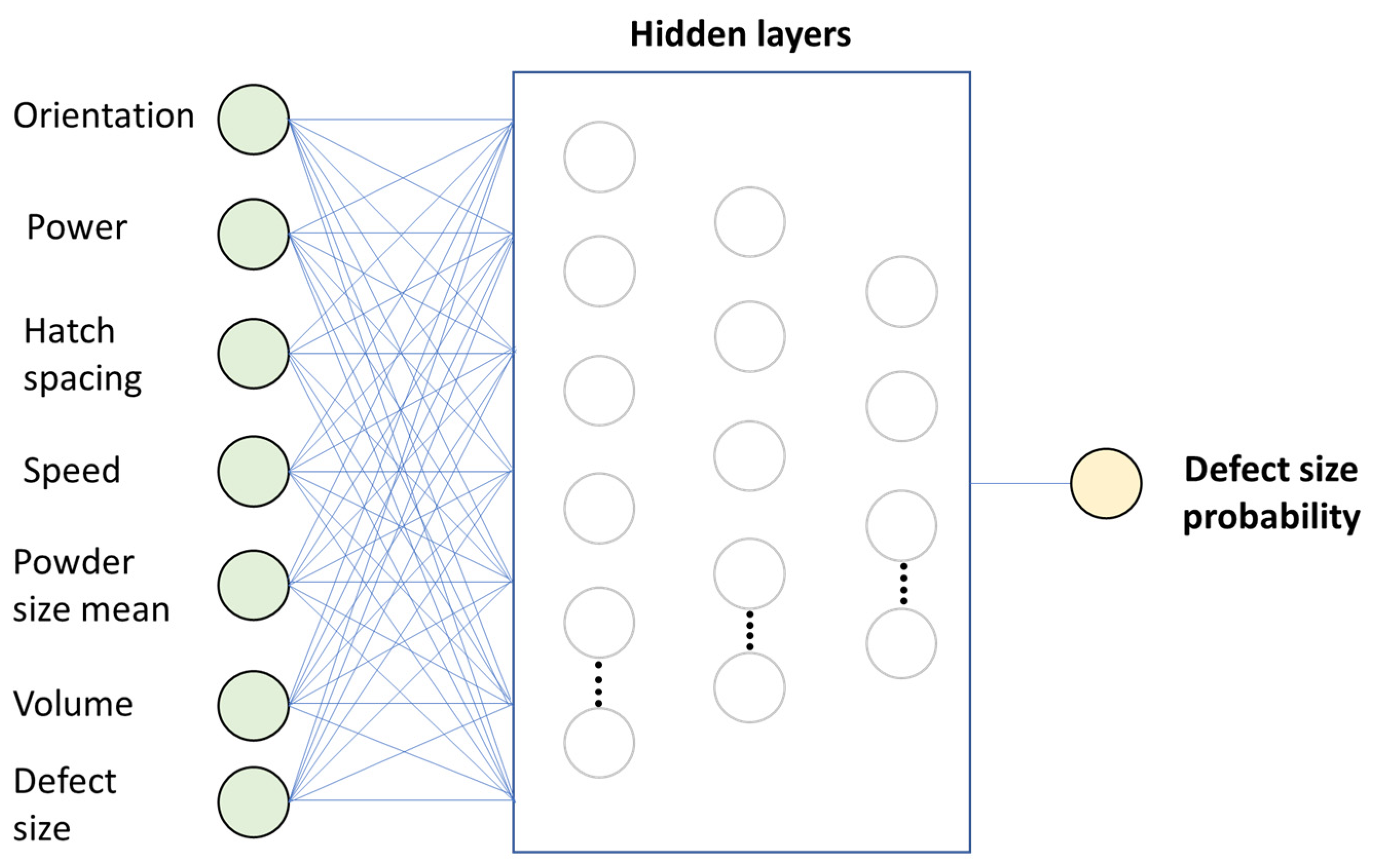
2.3.1. NN Architecture: Probability of a Specific Defect Size (Probability ML)

The first developed ML algorithm, the Probability ML algorithm in the following, provides in output the probability of a defect with size $\sqrt{a_c}$. Accordingly, the input parameters are the SLM process parameters, the defect size $\sqrt{a_c}$ and the risk-volume V₉₀. Figure 2 visualizes the input parameters and the output of the developed ML algorithms.

The developed NN is composed of three hidden layers and one output layer, the first one with 100 neurons, the second one with 75 neurons and the third one with 50 neurons. The number of hidden layers has been optimized to maximize the NN performance. Accordingly, the number of hidden layers has been varied to find the configuration minimizing the loss function for the set of the other selected hyperparameters. For each hidden layer, the hyperbolic tangent activation function has been used, whereas for the output layer a linear activation function has been considered. The activation functions have been carefully chosen to provide the best performance and to minimize the average loss function. The other hyperparameters have been optimized depending on the material considered for the validation.

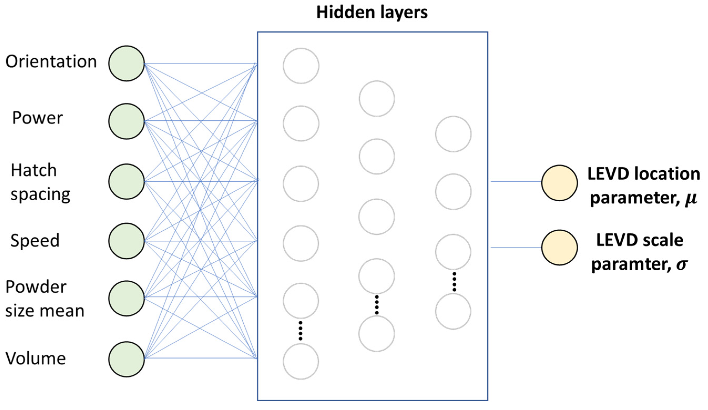
2.3.2. NN Architecture: LEVD Distribution Parameters (LEVD ML)

In the second developed ML algorithm, LEVD ML algorithm in the following, the input parameters are the process parameters and the risk volume, whereas the output parameters are the location and the scale parameters of the LEVD followed by $\sqrt{a_c}$. Figure 3 shows the input parameters and the output of the developed LEVD ML algorithm.

Even for this second approach, the NN is composed of three hidden layers and an output layer, the first one with 100 neurons, the second one with 75 neurons and the third one with 50 neurons. The number of hidden layers has been optimized to maximize the NN performance. Accordingly, the number of hidden layers has been varied to find the configuration minimizing the loss function for the set of the other selected hyperparameters. For each hidden layer, the hyperbolic tangent activation function has been used, whereas for the output layer a linear activation function has been considered. The activation functions have been carefully chosen to provide the best performance and to minimize the average loss function. The other hyperparameters have been optimized depending on the material considered for the validation.

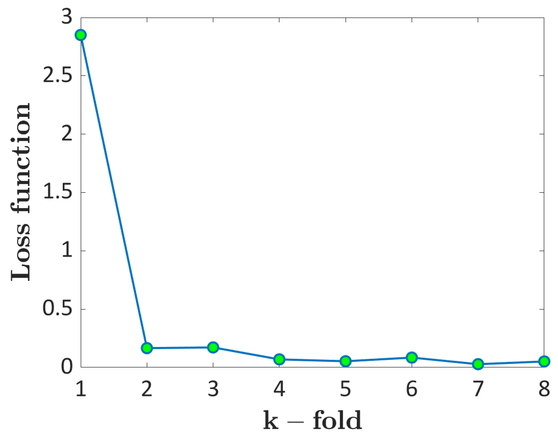
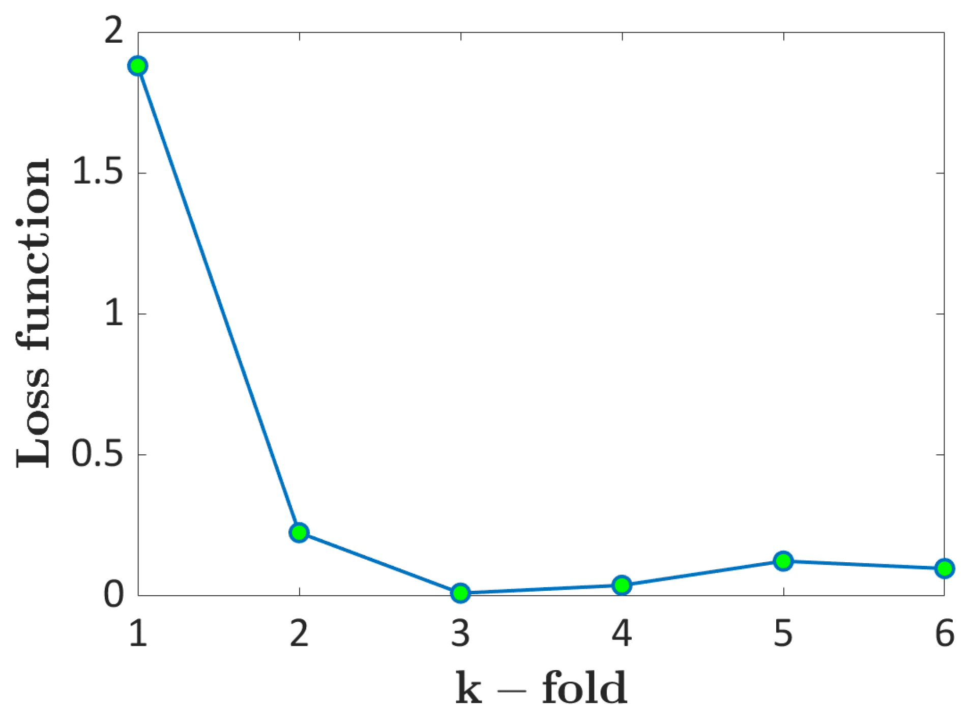
2.4. k-Fold Cross Validation

The predicting capability of the developed ML algorithms has been validated with a k-fold cross-validation procedure. Indeed, ML algorithms can be effectively employed only if it can be shown that they can predict the output on datasets that have not been used for the training. k-fold cross-validation ensures a reliable validation, especially for a limited number of available data. According to this procedure, the input dataset is divided into k subsets of data, called folds. The model is thereafter trained on all folds except one, i.e., k − 1 folds, and thereafter the loss function is computed on the subset not used for the training process. This resampling procedure provides an appropriate and reliable validation of the ML algorithm and ensures that each fold is used as the validation dataset. The training process is therefore iteratively repeated. For example, by considering five folds, the dataset is subdivided into five folds. In the first iteration, the first fold (k = 1) is used as the test dataset, whereas the other k − 1 folds are used as the training dataset. In the second iteration, the second fold (k = 2) is used as the test dataset, whereas the other k − 1 folds are used as the training dataset. The procedure ended when each fold is used as the testing dataset. Figure 4 helps to clarify the k-fold cross-validation procedure, by considering five folds.

3. Experimental Validation

In this Section, the ML algorithms described in Section 2 are validated using experimental data from the literature. Section 3.1 focuses on the validation on SLM AlSi10Mg data, whereas Section 3.2 focuses on the validation of SLM Ti6Al4V literature data.

The experimental data for the AlSi10Mg and the Ti6Al4V alloy have been digitized with the software Engauge from images in the original papers, if not available in tabular form. For the analysis, literature papers, where the defect sizes and the process parameters described in Section 2.2 were available, have been considered. Since the focus of the proposed approaches are the critical defects, i.e., those controlling the fatigue response and from which the crack initiates, defects at the origin of the fatigue failures after experimental tests have been considered. The risk-volume of dog-bone specimens subjected to conventional fatigue axial tests has been computed analytically by considering the gage section and the gage length. The risk-volume of hourglass specimens subjected to conventional axial fatigue tests or of specimens subjected to ultrasonic fatigue tests has been computed through Finite Element Analyses (FEAs), starting from the specimen geometry reported in the original paper. For the validation of the LEVD ML approach, the location and scale parameters of the original datasets and for a given set of process parameters have been estimated by applying the Maximum Likelihood Principle and by considering the LEVD truncated to 0 $\mathsf{\mu }\mathrm{m}$, i.e., by implying that defects cannot have a negative size, according to [31]. The experimental probabilities for the defect sizes contained in each dataset have been computed with Benard’s approximation for Median Ranks [32].

In the following analyses, the number of folds has been selected depending on the datasets and on the number of available data, to have enough data for an effective training and a reliable validation. Accordingly, for the Probability ML the number of folds has been selected to have at least 24 data for the validation, whereas for the LEVD ML the number of folds has been selected to have at least two datasets within each validation fold for the majority number of folds (in particular, due to the number of available datasets, three folds for the Ti6Al4V alloy have one dataset for the validation). The split ratio between training and validation data is given by the reciprocal of the number of folds.

For the sake of clarity, in the following figures for the validation of the Probability ML algorithm, “ML predicted” refers to the probabilities predicted with the Probability ML, whereas “Experimental” refers to the experimental probability. In the figure for the validation of the LEVD ML, “Experimental fit” and “ML fit” refers to the LEVD estimated experimentally and with the developed ML algorithm, respectively.

3.1. AlSi10Mg Validation

This Section focuses on the validation of the Probability ML and LEVD ML algorithms on SLM AlSi10Mg datasets [30,33,34,35,36]. In Figure 5, the experimental datasets considered for the validation are reported in a Gumbel plot.

According to Figure 5, the experimental defects show a large scatter, thus highlighting the influence of the investigated process parameters on the fatigue response and justifying the use of ML algorithms for solving this problem concerning the structural integrity of SLM parts. Defects are characterized by sizes ranging from 40 $\mathsf{\mu }\mathrm{m}$ up to 1000 $\mathsf{\mu }\mathrm{m}$, even if only two datasets out of twenty show defects with sizes above 400 $\mathsf{\mu }\mathrm{m}$. The defects in [30] were experimentally obtained by the authors. The data in [34,35] were available in tabular form. The experimental data in [36] were randomly simulated starting from the parameters of the LEVD distribution for machined specimens. Therefore, for these experimental data, a “digitization error” is excluded. On the other hand, the experimental datasets in [33] were retrieved by using the Engauge Digitizer software. A digitization error cannot be excluded for these datasets. However, it should be noted that the objective of Section 3 is to validate Machine Learning algorithms and a small error in the digitization of the defect size can be accepted, having limited influence on the validation process.

Table 1. Range of process parameters for the datasets on AlSi10Mg considered for the validation of the developed ML algorithms.

Orientation	Power	Speed	Hatch Distance	Layer Thickness	Average Powder Size	Risk Volume
	[W]	[mm/s]	[$\mathsf{\mu }\mathrm{m}]$	[$\mathsf{\mu }\mathrm{m}]$	[$\mathsf{\mu }\mathrm{m}$]	[mm3]
[0, 90]	[220, 380]	[600, 1650]	[130, 190]	[30, 60]	[30, 41.5]	[250, 2300]

summarizes the process parameter and the risk-volume ranges of the investigated datasets.

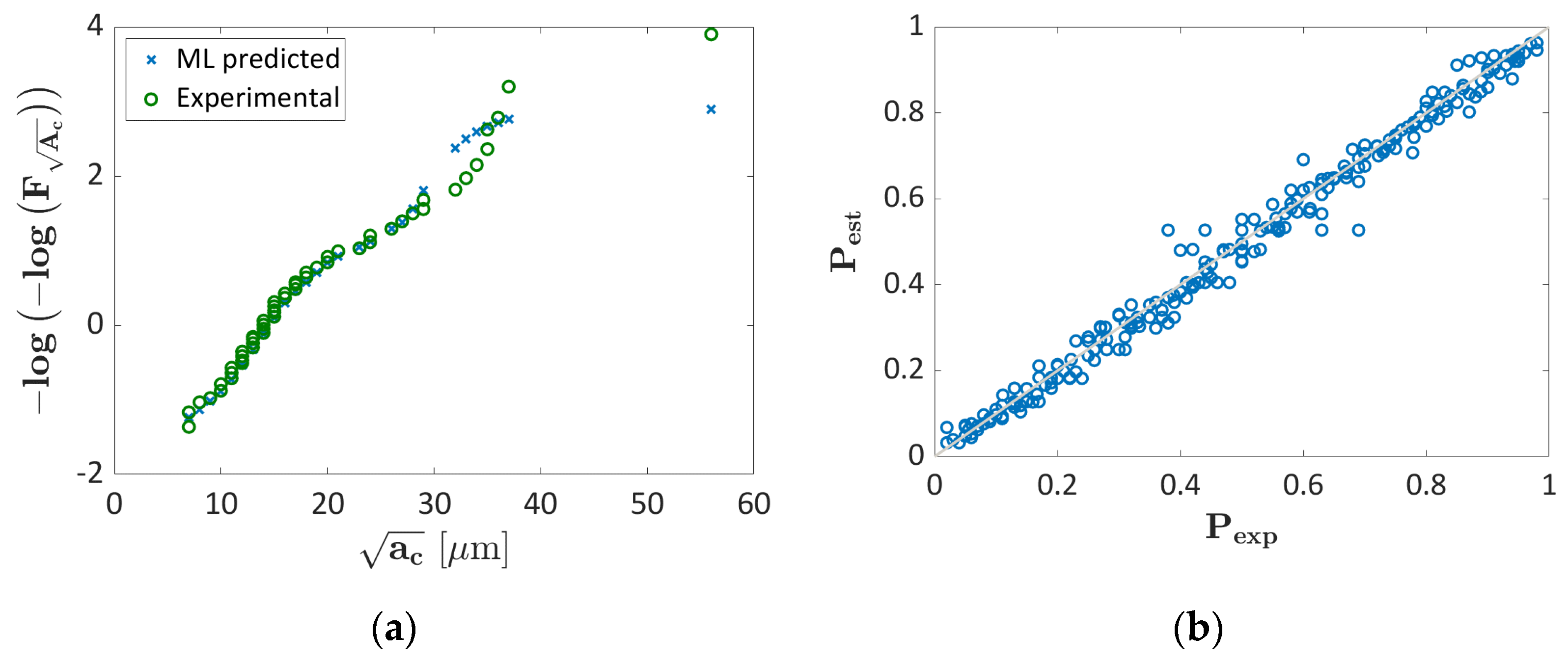
3.1.1. Probability ML Validation

In this Section, the Probability ML approach is validated. Figure 6 plots the loss function in function of the k-fold considered for the validation. For example, k = 3 means that the third subset has been considered as the validation dataset. According to the k-fold validation scheme, the data available in each validation fold is at least 24, thus providing a reliable validation.

According to Figure 6, the trend is almost constant and flat, with the loss function below 0.2 for all folds, except for the first one, characterized by a loss function above 2.5. This means that the developed ML algorithm works well for the investigated dataset, but for one fold, it has a low predicting capability.

Figure 7 shows the Gumbel plot for the validation (Figure 7a) fold and a training fold (Figure 7b) for k = 1, i.e., the validation fold for which the loss function reaches its maximum value and where the Probability ML shows, therefore, its worst performance.

According to Figure 7a, the predicted probabilities are not conservative, with the Probability ML algorithm providing larger probabilities and with the predicted data above the experimental data. Indeed, the ML-predicted probability of a defect smaller than $\sqrt{a_c}$ is larger (with therefore a smaller probability of defects with a size larger than $\sqrt{a_c}$), being theML predictions less-safe. The percent error, i.e., the difference between the predicted probability and the experimental one, normalized by the experimental probability has also been adopted to quantify the error in the prediction. The percentage error has been found in the range [5.2, 1310]%, with a median value of 94%. As expected, the percentage error is very large, especially for small defect sizes where it reaches its maximum. Indeed, the difference range reduces to [5.2, 605]%, with the median value equal to 81%, without considering the smallest defect. However, it must be noted that this validation dataset is the one showing anomalous behavior, i.e., the one with defects significantly larger than those found in other datasets (Figure 5). This could be the reason for the large differences in Figure 7a and the predicting capability can be enhanced by increasing the number of training datasets covering the range of $\sqrt{a_c}$ above 400 $\mathsf{\mu }\mathrm{m}$. On the other hand, the ML and the experimental probabilities for the training dataset in Figure 7b overlap, with negligible differences (percent difference in the range [0.6, 15.6]%, with a median value equal to 2.4).

Figure 8 shows the Gumbel plots for the validation dataset for k = 4, i.e., one of the validation folds characterized by a loss function below 0.2. Figure 8b shows the Probability–Probability plot, with the abscissa axis reporting the experimental probability, P_exp, and the ordinate axis reporting the probability estimated with the ML algorithm, P_est, for k = 4 and by considering the training and the validation data.

According to Figure 8a, the ML probabilities are in good agreement with the experimental data for k = 4, with limited differences. The percent difference is in the range [2.5, 212.5]%, with a median value of 64%. Unexpectedly, the range is quite large, with the largest differences found for defects smaller than 40 $\mathsf{\mu }$m. Indeed, if the defects smaller than 40 $\mathsf{\mu }$m are not considered, the range is significantly reduced, i.e., [2.5, 51]%, with the median value equal to 13%, proving that the Probability ML has high predicting capabilities, with however possible small deviations in specific defect size ranges. Since other validation folds are characterized by similar loss functions, it can be concluded that the Probability ML algorithm also performs properly for them. The probability plot in Figure 8b further confirms the validity of the developed approach, with all the training and validation data concentrated close to the bisector.

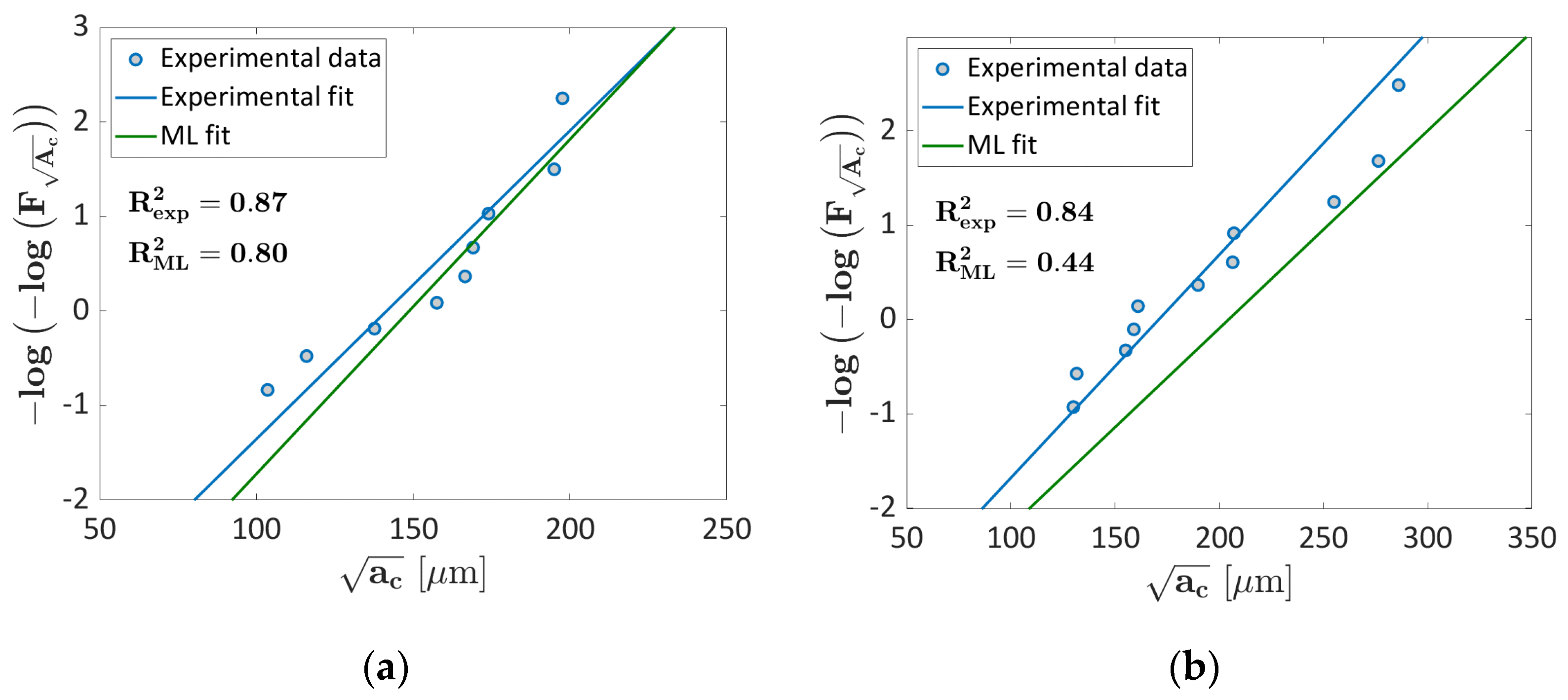
3.1.2. LEVD ML Algorithm: Validation

In this Section, the LEVD ML algorithm (Section 2.3.2) is validated on AlSi10Mg data. Figure 9 plots the loss function with respect to the k-fold considered for the validation.

According to Figure 9, the loss function is almost flat and below 0.2 for all the considered folds, except for fourth fold. Accordingly, the LEVD ML has averagely good predicting capabilities on validation datasets.

Figure 10 shows the Gumbel plot for the validation (Figure 10a) and a training (Figure 10b) fold for k = 4, i.e., the validation fold for which the loss function reaches its maximum. In Figure 10 and in the following Figures, $R_{exp}^2$ and $R_{ML}^2$ refer to the coefficient of determination computed by considering the experimental fit and the ML fit, respectively.

According to Figure 10a, the ML LEVD is in good agreement with the experimental LEVD and provides an acceptable prediction, even if characterized by a higher slope. The $R_{exp}^2$ and $R_{ML}^2$ are very close, being equal to 0.94 and 0.93, respectively, thus confirming the effectiveness of the prediction. The predictive capability of this approach can be further improved by increasing the number of datasets available for the training. The experimental and the ML LEVD for the training dataset are close and tend to overlap, providing the same $R_{exp}^2$ and $R_{ML}^2$ values.

An interesting further validation can be carried out by verifying the capability of the ML algorithm of predicting the LEVD variation with the risk-volume, and thus of modelling size effect. This can be done by considering the dataset in [30]. Indeed, experimental tests in [30] have been carried out on specimens produced with the same process parameters, but with horizontal and vertical building orientations and with different risk volumes (200 mm³ and 2300 mm³). Figure 11 shows the Gumbel plot of experimental data in [30] for defects measured on the fracture surfaces of specimens built in a horizontal (Figure 11a) and vertical direction (Figure 11b) and with a risk volume of 2300 mm³. These are the validation datasets for k = 2 (Figure 11a) and k = 3 (Figure 11b), and therefore have not been considered for the training. In Figure 11, the blue line is the LEVD estimated from the experimental data, whereas the green line is the ML LEVD.

According to Figure 11, the predicted LEVDs are in good agreement with the experimental data and with experimental LEVD. In Figure 11a, $R_{exp}^2$ and $R_{ML}^2$ are close and are equal to 0.87 and 0.80, respectively. The percent differences between the location and the scale parameters, computed as the difference between the experimental and the ML values, normalized by the experimental values, are equal to 5.1% and 7.8%, respectively. The difference tends to be larger for vertical specimens (Figure 11b), for which $R_{exp}^2$, equal to 0.84, is larger than the $R_{ML}^2$ value, equal to 0.44. This decrement can be explained by analyzing the percentage difference between the location and the scale parameters, equal to 19.6% and 12.8%, respectively, with the ML fit being shifted rightward with respect to the experimental curve. However, in both cases, the predicted values are close to the experimental ones and the differences are in an acceptable range. This validation confirms the capability of the LEVD ML algorithm of modelling size effect, which has a fundamental importance when components are designed, since datasets on defect size are obtained with experimental tests on specimens with small volumes, whereas components are characterized by significantly larger risk volumes.

3.2. Ti6Al4V Validation

In this Section, the ML models are further validated by considering datasets on Ti6Al4V alloy specimens [28,37,38,39,40,41]. Figure 12 plots the defect sizes in a Gumbel plot for the datasets considered for training and validating the NN. The investigated datasets show a large scatter, thus proving the influence of the process parameters on the defect size. The data in [40,41] were available in tabular form, whereas the experimental datasets in [28,37,38,39] were retrieved by using the Engauge Digitizer software. As for the AlSi10Mg alloy, errors in the digitization are small and have limited influence in the validation process.

In particular, defects are concentrated below 150 $\mathsf{\mu }\mathrm{m}$, except for one dataset, characterized by defects with equivalent size up to 400 $\mathsf{\mu }\mathrm{m}$.

Table 2. Range of process parameters for the datasets on Ti6Al4V considered for the validation of the developed ML algorithms.

Orientation	Power	Speed	Hatch Distance	Layer Thickness	Average Powder Size	Risk Volume
	[W]	[mm/s]	[$\mathsf{\mu }\mathrm{m}]$	[$\mathsf{\mu }\mathrm{m}]$	[$\mathsf{\mu }\mathrm{m}$]	[mm3]
[0, 90]	[175, 400]	[150, 1400]	[120, 140]	[30, 60]	[34, 45]	[84, 1204]

summarizes the process parameter and the risk-volume ranges of the investigated datasets.

3.2.1. Probability ML Validation

In this Subsection, the Probability ML algorithm has been validated. Figure 13 plots the loss function with respect to the k-fold considered for the validation. As for the AlSi10Mg alloy, the trend is almost constant, with the loss function being flat and below 0.25, except for the first fold, characterized by a significantly higher value, above 1.75.

In order to stress the fitting capability of the ML algorithm in the worst condition, the validation and the training dataset for the first k-fold have been considered. Figure 14 shows the Gumbel plot for the k = 1 fold, Figure 14a shows the Gumbel plot for the validation fold, whereas Figure 14b shows the Gumbel plot for a training fold.

According to Figure 14, the trend predicted with the Probability ML is similar to the experimental one, but the data are significantly above, being less conservative. The percentage difference is in a large range, [4.8, 1289]%, with a median value equal to 94%, as expected. In particular, for defects characterized by small size, the difference tends to be higher and justifies the large percentage difference range. It must be noted that, as for the AlSi10Mg alloy, the Probability ML has quite poor predictive capability for the validation dataset showing an anomalous trend with respect to the other datasets considered for the training. This criticality in the prediction can be overcome by increasing the number of datasets with defects in the range [150–400] µm. On the other hand, according to Figure 14b, the estimated ML probabilities are in good agreement with the experimental ones for a training dataset, as for the AlSi10Mg alloy, with the median percentage difference equal to 2.8%.

Figure 15a shows the Gumbel plot for the k = 3 validation fold, i.e., a fold characterized by a small loss factor. Figure 15b, shows, on the other hand, the Probability–Probability plot, with the abscissa axis reporting the experimental probability, P_exp, and the ordinate axis the ML probability, P_est.

According to Figure 15a, the predicted and the experimental data are in good agreement, thus confirming the predicting capability of the proposed method for the range of defect size where many data are available for the training. The largest percentage difference, equal to 60%, has been found for the largest experimental defect, but the median percentage difference is very small, being about 4.7%. As for the AlSi10Mg alloy, the Probability ML has, on average, very good predictive capabilities, with larger deviations only for specific defect sizes or defect sizes ranges. Since for the other validation k-folds the loss factor has almost the same value, it can be reasonably inferred that the developed ML algorithm also works properly for them. The P–P plot further confirms the validity of this approach, with all the data concentrated close to the bisectors.

3.2.2. LEVD ML Algorithm Validation

In this Section, the LEVD ML is validated using Ti6Al4V data. Figure 16 plots the loss function with respect to the k-fold considered for the validation. According to Figure 16, the computed validation loss functions are close to 0.04, with only the one computed for k = 1 showing a larger value close to 0.14.

The predictive capability has been thereafter verified on the validation fold for which the loss function shows the largest value, i.e., for k = 1. Figure 17 compares the LEVD computed experimentally and with the ML algorithm: Figure 17a for the validation dataset and Figure 17b for a training fold randomly chosen.

According to Figure 17a, the LEVD ML algorithm works well even for the first fold, i.e., for the dataset characterized by defects significantly larger than those found in the other datasets, for which the Probability ML has shown worse performance (Figure 14a). $R_{exp}^2$ and $R_{ML}^2$ are very close, being equal to 0.95 and 0.93. The slope and the intercept show acceptable differences, with the two curves showing similar trends. Accordingly, the LEVD ML has proven to work better than the Probability ML for the Ti6Al4V dataset showing an “anomalous” trend. As for the other analyses, the LEVD ML overlaps with the experimental LEVD for the training dataset (Figure 17b).

4. Discussion

In this Section, the architecture, as well as the input parameters, of the developed ML algorithms are analyzed and discussed, to highlight their strengths and weaknesses and point out possible improvements. It must be noted that the proposed ML algorithms have been developed to address a challenging open issue concerning the structural integrity and the design against the fatigue of AM components and to show that NN networks can be reliably employed in industrial and research fields. The methodologies analyzed in the Introduction section employ ML algorithms with this objective, but with a different approach. “Traditional” approaches, such as the one in [35] can be also considered for the sake of comparison. In [35], the process parameters are varied to assess their influence on the defect population. However, a model that provides the probability associated with a defect size directly from the process parameters has not been proposed yet and it can be hardly developed with this “traditional” approach, due to the unfeasible number of data required for a reliable estimation.

As pointed out in the Introduction Section, the surface roughness has not been considered in the present work, even if it is the factor that most affects the fatigue response. However, for the prediction of the surface roughness, a specific NN with additional inputs, such as surface treatments, should be considered. Similarly, the influence of the loading direction with respect to the building orientation has not been considered, since this work focuses on critical defects and it does not provide in its output the fatigue response. However, starting from the predicted defect size, which accounts for the influence of the building direction, and by considering damage-tolerant approaches, the effect of the load direction on the fatigue response of AM parts can be reliably modelled.

In this work, the most relevant SLM process parameters have been considered as input for the ML algorithms, generally reported in the literature papers on the fatigue response of SLM specimens. By analyzing the available datasets (Figure 5 and Figure 12), it must be noted that the scatter associated with the defect size is large, even for the same set of process parameters. Process parameters different from those considered in the present paper, or post-treatments, can be the reason for this large scatter or can influence the critical defect population. For example, heat treatments have not been considered as inputs for the ML algorithms, since the literature results agree that they do not affect the defect size, especially low-temperature heat treatments. However, the influence of heat treatments is still debated in the literature, since some researchers have proven that they can enlarge porosities [42,43]. Similarly, heating the building platform helps to stabilize the melt pool [44], with a positive effect on the defect size and with the part being more “damage tolerant” [45]. Moreover, in place of the average powder size, the powder size range can be considered as input. Indeed, a large dispersion of the powder size could induce the formation of larger defects and this cannot be accounted for by considering the average powder size. Other “hidden” factors can also contribute to the defect size scatter observed in Figure 5 and Figure 12 and may have stressed the predictive capability of the developed ML algorithms. For example, the AM production systems can influence the defect size population, providing different defect sizes, even for the same set of process parameters. All these factors, which are known to have a smaller influence on the defect population, can, however, contribute to the large experimental scatter and can be integrated into the ML algorithms to improve their predictive capability, provided that significantly larger datasets are available and can be used for a reliable training process.

The influence of defect location has not been considered in the present work, since the NN algorithms have been trained to predict the defect sizes, regardless of their location. However, the defect location has a significant influence on the fatigue response, with surface defects being more critical. An effective approach for modelling the larger criticality of surface defects is to multiply the defect size predicted with the developed NN by the ratio between the Stress Intensity Factor (SIF) associated with a surface defect and the SIF of an internal defect (i.e., 0.65/0.5=1.3). Accordingly, the predicted defect is considered as an internal defect and its equivalent size can be increased by a factor of 1.3 for the design with damage-tolerant approaches against surface defect failures, i.e., to model the largest criticality associated with surface defects with a reliable fracture mechanics approach.

The Probability and the LEVD ML algorithms have confirmed their effectiveness in the proposed architecture, as demonstrated by the validation using two of the most used SLM materials, the AlSi10Mg and the Ti6Al4V alloy. The loss functions computed for the validation datasets were shown to be almost constant for both approaches and materials, apart, in general, from one validation dataset. However, it is widely known that the predicting capability tends to decrease for datasets characterized by large differences with respect to the other available datasets, since the ML algorithm is required to predict the defect probabilities or the LEVD parameters outside the domain explored by the training data (Figure 7a and Figure 14a). The LEVD ML algorithm has proven to work better for this type of dataset, as confirmed by comparing Figure 14a and Figure 17a for the Ti6Al4V alloy dataset (validation fold for k = 1). Indeed, the Probability ML algorithm has overestimated the probability associated with each defect, whereas the LEVD has provided good predictions, with limited differences in the slope and the intercept. For the Probability ML, the number of training data is larger (one probability for each defect and set of process parameters for the Probability ML, the location and the scale parameters for each dataset for the LEVD ML), enhancing the predictive capability of the NN. On the other hand, this approach does not ensure that, given the same set of process parameters, larger defects will be characterized by larger probabilities, violating the physical linearly increasing trend on the Gumbel plot. This is a limitation of the Probability ML algorithm, as shown in Figure 14a, which may be overcome by increasing the number of training data. On the other hand, the LEVD ML embeds a statistical model based on experimental evidence, thus overcoming this criticality and providing better predictions.

To conclude, the proposed approaches can be reliably used to address this important subject concerning the structural integrity of AM components. It must be noted that more complex models and architectures dealing with reliability analysis [46,47,48,49] may have also been used. However, the proposed algorithms, despite their simple architecture, properly and reliably work for two of the most used SLM materials, the AlSi10Mg and the Ti6Al4V alloy, even for a number of available data for the training that is smaller than that generally considered for this kind of algorithms. The performances of the developed NN are expected to be further enhanced by increasing the number of literature data, especially in the defect size ranges where data are missing, without the need for further complicating their architecture.

5. Conclusions

In this paper, two Machine Learning (ML) algorithms, supervised feed-forward neural networks (FFNNs), have been developed for the analysis of the critical manufacturing defects in components to be produced by Selective Laser Melting (SLM). The first one provides in output the probability associated with a specific defect starting from the main process parameters and the part risk-volume (Probability ML in the following). The second one estimates the location and the scale parameter of the defect size distribution, assumed to follow the Largest Extreme Value Distribution (LEVD), receiving in input the main process parameters and the part volume (LEVD ML in the following). The process parameters considered in input are those mainly affecting the defect population and the fatigue response, i.e., the building orientation, the input power, the scan speed, the hatch distance, the layer thickness and the average powder size. The predicting capability has been verified using literature datasets obtained with tests on AlSi10Mg and Ti6Al4V alloys.

The following conclusions can be drawn:

• Probability ML and LEVD ML have shown a high predicting capability for both AlSi10Mg and Ti6Al4V datasets. A k-fold cross-validation scheme has been used for the validation, proving that both approaches can be reliably used for the analysis of defects in SLM components. The loss functions with respect to the fold considered for the validation were almost constant, thus confirming the good performances of both architectures.
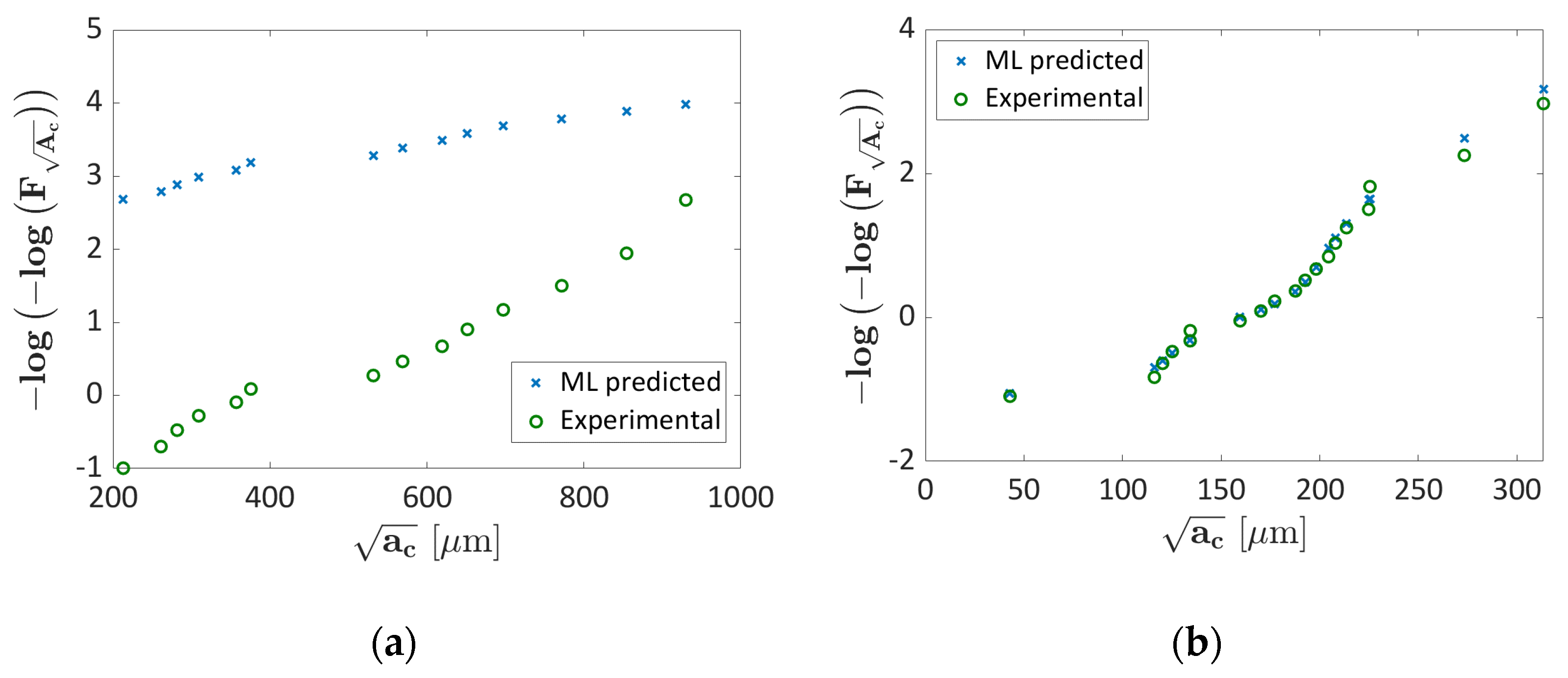
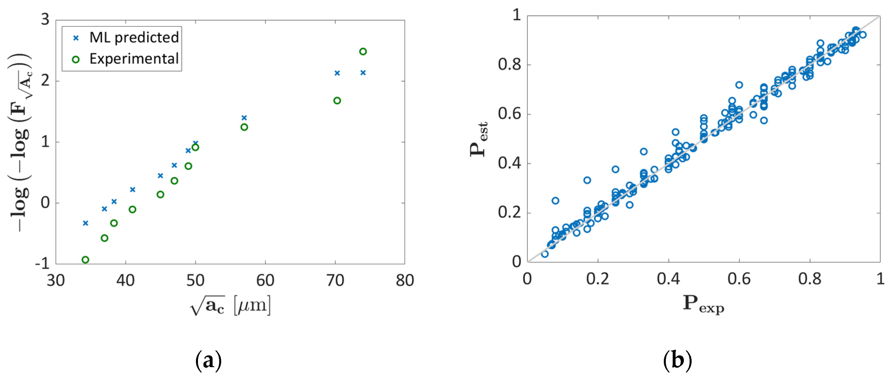
• LEVD ML has been shown to work well even for datasets with a trend significantly different from that of the other datasets considered for the training process. On the other hand, the Probability ML algorithm tends to overestimate the probability associated with each defect, being less conservative.
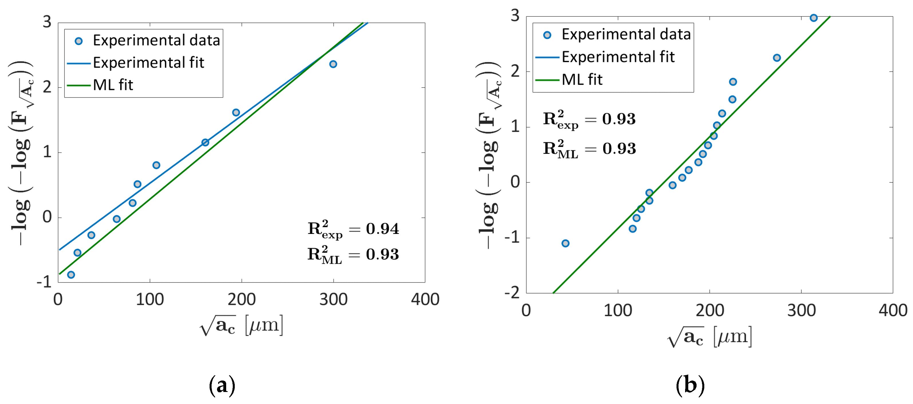
• The trend in the Gumbel Plot estimated with the Probability ML algorithm can show a large scatter and, for the same process parameters, it is not ensured that larger defects are characterized by larger probabilities. This can be solved by increasing the number of training data. On the other hand, the LEVD ML “embeds” the LEVD statistical model based on the experimental evidence, thus overcoming this criticality.
• The predicting capability of both developed ML algorithms may be enhanced by adding more input factors, whose influence on the defect size population is still debated in the literature, such as heat treatment temperature, the building platform heating temperature, the powder size ranges and the SLM production system. However, the number of available datasets for the training process should be significantly increased.

To conclude, this analysis has pointed out that the proposed ML algorithms can be reliably used for the prediction of the probability of specific defect sizes in SLM components and for the subsequent fatigue design with damage-tolerant approaches and, in general, that approaches based on ML should be used to ensure the structural integrity of AM components subjected to defect-driven fatigue failures.

References

1. Yadollahi, A.; Shamsaei, N. Additive Manufacturing of Fatigue Resistant Materials: Challenges and Opportunities. Int. J. Fatigue 2017, 98, 14–31. [Google Scholar] [CrossRef] [Green Version]
2. Mower, T.M.; Long, M.J. Mechanical Behavior of Additive Manufactured, Powder-Bed Laser-Fused Materials. Mater. Sci. Eng. A 2016, 651, 198–213. [Google Scholar] [CrossRef]
3. Uzan, N.E.; Shneck, R.; Yeheskel, O.; Frage, N. Fatigue of AlSi10Mg Specimens Fabricated by Additive Manufacturing Selective Laser Melting (AM-SLM). Mater. Sci. Eng. A 2017, 704, 229–237. [Google Scholar] [CrossRef]
4. Murakami, Y. Metal Fatigue: Effects of Small Defects and Nonmetallic Inclusions; Elsevier: Amsterdam, The Netherlands, 2002; ISBN 9780128138779. [Google Scholar]
5. Masuo, H.; Tanaka, Y.; Morokoshi, S.; Yagura, H.; Uchida, T. Influence of Defects, Surface Roughness and HIP on the Fatigue Strength of Ti-6Al-4V Manufactured by Additive Manufacturing. Int. J. Fatigue 2018, 117, 163–179. [Google Scholar] [CrossRef]
6. Sanaei, N.; Fatemi, A. Defects in Additive Manufactured Metals and Their Effect on Fatigue Performance: A State-of-the-Art Review. Prog. Mater. Sci. 2021, 117, 100724. [Google Scholar] [CrossRef]
7. Beretta, S.; Romano, S. A Comparison of Fatigue Strength Sensitivity to Defects for Materials Manufactured by AM or Traditional Processes. Int. J. Fatigue 2017, 94, 178–191. [Google Scholar] [CrossRef]
8. Romano, S.; Brückner-Foit, A.; Brandão, A.; Gumpinger, J.; Ghidini, T.; Beretta, S. Fatigue Properties of AlSi10Mg Obtained by Additive Manufacturing: Defect-Based Modelling and Prediction of Fatigue Strength. Eng. Fract. Mech. 2018, 187, 165–189. [Google Scholar] [CrossRef]
9. Tridello, A.; Boursier Niutta, C.; Berto, F.; Qian, G.; Paolino, D.S. Fatigue Failures from Defects in Additive Manufactured Components: A Statistical Methodology for the Analysis of the Experimental Results. Fatigue Fract. Eng. Mater. Struct. 2021, 44, 1944–1960. [Google Scholar] [CrossRef]
10. Zhang, M.; Sun, C.N.; Zhang, X.; Wei, J.; Hardacre, D.; Li, H. Predictive Models for Fatigue Property of Laser Powder Bed Fusion Stainless Steel 316L. Mater. Des. 2018, 145, 42–54. [Google Scholar] [CrossRef]
11. Du, L.; Qian, G.; Zheng, L.; Hong, Y. Influence of Processing Parameters of Selective Laser Melting on High-Cycle and Very-High-Cycle Fatigue Behaviour of Ti-6Al-4V. Fatigue Fract. Eng. Mater. Struct. 2021, 44, 240–256. [Google Scholar] [CrossRef]
12. Zhan, Z.; Li, H. A Novel Approach Based on the Elastoplastic Fatigue Damage and Machine Learning Models for Life Prediction of Aerospace Alloy Parts Fabricated by Additive Manufacturing. Int. J. Fatigue 2021, 145, 106089. [Google Scholar] [CrossRef]
13. Maleki, E.; Bagherifard, S.; Razavi, S.M.J.; Bandini, M.; du Plessis, A.; Berto, F.; Guagliano, M. On the Efficiency of Machine Learning for Fatigue Assessment of Post-Processed Additively Manufactured AlSi10Mg. Int. J. Fatigue 2022, 160, 106841. [Google Scholar] [CrossRef]
14. Chen, J.; Liu, Y. Fatigue Property Prediction of Additively Manufactured Ti-6Al-4V Using Probabilistic Physics-Guided Learning. Addit. Manuf. 2021, 39, 101876. [Google Scholar] [CrossRef]
15. Schneller, W.; Leitner, M.; Maier, B.; Grün, F.; Jantschner, O.; Leuders, S.; Pfeifer, T. Artificial Intelligence Assisted Fatigue Failure Prediction. Int. J. Fatigue 2022, 155, 106580. [Google Scholar] [CrossRef]
16. Salvati, E.; Tognan, A.; Laurenti, L.; Pelegatti, M.; De Bona, F. A Defect-Based Physics-Informed Machine Learning Framework for Fatigue Finite Life Prediction in Additive Manufacturing. Mater. Des. 2022, 222, 111089. [Google Scholar] [CrossRef]
17. Awd, M.; Münstermann, S.; Walther, F. Effect of Microstructural Heterogeneity on Fatigue Strength Predicted by Reinforcement Machine Learning. Fatigue Fract. Eng. Mater. Struct. 2022, 45, 3267–3287. [Google Scholar] [CrossRef]
18. Wang, H.; Li, B.; Xuan, F.Z. Fatigue-Life Prediction of Additively Manufactured Metals by Continuous Damage Mechanics (CDM)-Informed Machine Learning with Sensitive Features. Int. J. Fatigue 2022, 164, 107147. [Google Scholar] [CrossRef]
19. Ciampaglia, A.; Tridello, A.; Paolino, D.S.; Berto, F. Data Driven Method for Predicting the Effect of Process Parameters on the Fatigue Response of Additive Manufactured AlSi10Mg Parts. Int. J. Fatigue 2023, 170, 107500. [Google Scholar] [CrossRef]
20. Shi, T.; Sun, J.; Li, J.; Qian, G.; Hong, Y. Machine Learning Based Very-High-Cycle Fatigue Life Prediction of Ti-6Al-4V Alloy Fabricated by Selective Laser Melting. Int. J. Fatigue 2023, 173, 107585. [Google Scholar] [CrossRef]
21. Cutolo, A.; Lammens, N.; Vanden Boer, K.; Erdelyi, H.; Schulz, M.; Muralidharan, G.K.; Thijs, L.; Elangeswaran, C.; Van Hooreweder, B. Fatigue Life Prediction of a L-PBF Component in Ti-6Al-4V Using Sample Data, FE-Based Simulations and Machine Learning. Int. J. Fatigue 2023, 167, 107276. [Google Scholar] [CrossRef]
22. Colombo, C.; Tridello, A.; Pagnoncelli, A.P.; Biffi, C.A.; Fiocchi, J.; Tuissi, A.; Vergani, L.M.; Paolino, D.S. Efficient Experimental Methods for Rapid Fatigue Life Estimation of Additive Manufactured Elements. Int. J. Fatigue 2023, 167, 107345. [Google Scholar] [CrossRef]
23. Tridello, A.; Fiocchi, J.; Biffi, C.A.; Chiandussi, G.; Rossetto, M.; Tuissi, A.; Paolino, D.S. Effect of Microstructure, Residual Stresses and Building Orientation on the Fatigue Response up to 109 Cycles of an SLM AlSi10Mg Alloy. Int. J. Fatigue 2020, 137, 105659. [Google Scholar] [CrossRef]
24. Qian, G.; Li, Y.; Paolino, D.S.; Tridello, A.; Berto, F.; Hong, Y. Very-High-Cycle Fatigue Behavior of Ti-6Al-4V Manufactured by Selective Laser Melting: Effect of Build Orientation. Int. J. Fatigue 2020, 136, 105628. [Google Scholar] [CrossRef]
25. Mukherjee, S.; Kar, S.K.; Sivaprasad, S.; Tarafder, S.; Viswanathan, G.B.; Fraser, H.L. Creep-Fatigue Response, Failure Mode and Deformation Mechanism of HAYNES 282 Ni Based Superalloy: Effect of Dwell Position and Time. Int. J. Fatigue 2022, 159, 106820. [Google Scholar] [CrossRef]
26. Tang, M.; Pistorius, P.C. Fatigue Life Prediction for AlSi10Mg Components Produced by Selective Laser Melting. Int. J. Fatigue 2019, 125, 479–490. [Google Scholar] [CrossRef]
27. Fischer, C.; Schweizer, C. Lifetime Assessment of the Process-Dependent Material Properties of Additive Manufactured AlSi10Mg under Low-Cycle Fatigue Loading. MATEC Web Conf. 2020, 326, 07003. [Google Scholar] [CrossRef]
28. Soltani-Tehrani, A.; Habibnejad-Korayem, M.; Shao, S.; Haghshenas, M.; Shamsaei, N. Ti-6Al-4V Powder Characteristics in Laser Powder Bed Fusion: The Effect on Tensile and Fatigue Behavior. Addit. Manuf. 2022, 51, 102584. [Google Scholar] [CrossRef]
29. Jian, Z.M.; Qian, G.A.; Paolino, D.S.; Tridello, A.; Berto, F.; Hong, Y.S. Crack Initiation Behavior and Fatigue Performance up to Very-High-Cycle Regime of AlSi10Mg Fabricated by Selective Laser Melting with Two Powder Sizes. Int. J. Fatigue 2021, 143, 106013. [Google Scholar] [CrossRef]
30. Tridello, A.; Fiocchi, J.; Biffi, C.A.; Rossetto, M.; Tuissi, A.; Paolino, D.S. Size-Effects Affecting the Fatigue Response up to 109 Cycles (VHCF) of SLM AlSi10Mg Specimens Produced in Horizontal and Vertical Directions. Int. J. Fatigue 2022, 160, 106825. [Google Scholar] [CrossRef]
31. Paolino, D.S. Very High Cycle Fatigue Life and Critical Defect Size: Modeling of Statistical Size Effects. Fatigue Fract. Eng. Mater. Struct. 2021, 44, 1209–1224. [Google Scholar] [CrossRef]
32. Benard, A.; Bos-Levenbach, E.C. The Plotting of Observations on Probability Paper. Stat. Afd. 1953, 7, 163–173. [Google Scholar]
33. Wu, Z.; Wu, S.; Bao, J.; Qian, W.; Karabal, S.; Sun, W.; Withers, P.J. The Effect of Defect Population on the Anisotropic Fatigue Resistance of AlSi10Mg Alloy Fabricated by Laser Powder Bed Fusion. Int. J. Fatigue 2021, 151, 106317. [Google Scholar] [CrossRef]
34. Muhammad, M.; Nezhadfar, P.D.; Thompson, S.; Saharan, A.; Phan, N.; Shamsaei, N. A Comparative Investigation on the Microstructure and Mechanical Properties of Additively Manufactured Aluminum Alloys. Int. J. Fatigue 2021, 146, 106165. [Google Scholar] [CrossRef]
35. Rhein, R.K.; Shi, Q.; Arjun Tekalur, S.; Wayne Jones, J.; Carroll, J.W. Effect of Direct Metal Laser Sintering Build Parameters on Defects and Ultrasonic Fatigue Performance of Additively Manufactured AlSi10Mg. Fatigue Fract. Eng. Mater. Struct. 2021, 44, 295–305. [Google Scholar] [CrossRef]
36. Sausto, F.; Tezzele, C.; Beretta, S. Analysis of Fatigue Strength of L-PBF AlSi10Mg with Different Surface Post-Processes: Effect of Residual Stresses. Metals 2022, 12, 898. [Google Scholar] [CrossRef]
37. Günther, J.; Krewerth, D.; Lippmann, T.; Leuders, S.; Tröster, T.; Weidner, A.; Biermann, H.; Niendorf, T. Fatigue Life of Additively Manufactured Ti–6Al–4V in the Very High Cycle Fatigue Regime. Int. J. Fatigue 2017, 94, 236–245. [Google Scholar] [CrossRef]
38. Hu, Y.N.; Wu, S.C.; Withers, P.J.; Zhang, J.; Bao, H.Y.X.; Fu, Y.N.; Kang, G.Z. The Effect of Manufacturing Defects on the Fatigue Life of Selective Laser Melted Ti-6Al-4V Structures. Mater. Des. 2020, 192, 108708. [Google Scholar] [CrossRef]
39. Le, V.D.; Pessard, E.; Morel, F.; Edy, F. Interpretation of the Fatigue Anisotropy of Additively Manufactured TA6V Alloys via a Fracture Mechanics Approach. Eng. Fract. Mech. 2019, 214, 410–426. [Google Scholar] [CrossRef] [Green Version]
40. Alegre, J.M.; Díaz, A.; García, R.; Peral, L.B.; Cuesta, I.I. Effect of HIP Post-Processing at 850 °C/200 MPa in the Fatigue Behavior of Ti-6Al-4V Alloy Fabricated by Selective Laser Melting. Int. J. Fatigue 2022, 163, 107097. [Google Scholar] [CrossRef]
41. Hu, Y.N.; Wu, S.C.; Wu, Z.K.; Zhong, X.L.; Ahmed, S.; Karabal, S.; Xiao, X.H.; Zhang, H.O.; Withers, P.J. A New Approach to Correlate the Defect Population with the Fatigue Life of Selective Laser Melted Ti-6Al-4V Alloy. Int. J. Fatigue 2020, 136, 105584. [Google Scholar] [CrossRef]
42. Siddique, S.; Imran, M.; Walther, F. Very High Cycle Fatigue and Fatigue Crack Propagation Behavior of Selective Laser Melted AlSi12 Alloy. Int. J. Fatigue 2017, 94, 246–254. [Google Scholar] [CrossRef]
43. Schneller, W.; Leitner, M.; Leuders, S.; Sprauel, J.M.; Grün, F.; Pfeifer, T.; Jantschner, O. Fatigue Strength Estimation Methodology of Additively Manufactured Metallic Bulk Material. Addit. Manuf. 2021, 39, 101688. [Google Scholar] [CrossRef]
44. Tenkamp, J.; Awd, M.; Siddique, S.; Starke, P.; Walther, F. Fracture–Mechanical Assessment of the Effect of Defects on the Fatigue Lifetime and Limit in Cast and Additively Manufactured Aluminum–Silicon Alloys from Hcf to Vhcf Regime. Metals 2020, 10, 943. [Google Scholar] [CrossRef]
45. Santos Macías, J.G.; Douillard, T.; Zhao, L.; Maire, E.; Pyka, G.; Simar, A. Influence on Microstructure, Strength and Ductility of Build Platform Temperature during Laser Powder Bed Fusion of AlSi10Mg. Acta Mater. 2020, 201, 231–243. [Google Scholar] [CrossRef]
46. Zhuang, L.; Xu, A.; Wang, X.L. A Prognostic Driven Predictive Maintenance Framework Based on Bayesian Deep Learning. Reliab. Eng. Syst. Saf. 2023, 234, 109181. [Google Scholar] [CrossRef]
47. Jiao, Z.; Wang, H.; Xing, J.; Yang, Q.; Yang, M.; Zhou, Y.; Zhao, J. A LightGBM Based Framework for Lithium-Ion Battery Remaining Useful Life Prediction Under Driving Conditions. IEEE Trans. Ind. Inform. 2023. [Google Scholar] [CrossRef]
48. Luo, C.; Shen, L.; Xu, A. Modelling and Estimation of System Reliability under Dynamic Operating Environments and Lifetime Ordering Constraints. Reliab. Eng. Syst. Saf. 2022, 218, 108136. [Google Scholar] [CrossRef]
49. Chen, Z.; Zhou, D.; Zio, E.; Xia, T.; Pan, E. A Deep Learning Feature Fusion Based Health Index Construction Method for Prognostics Using Multiobjective Optimization. IEEE Trans. Reliab. 2022, 1–15. [Google Scholar] [CrossRef]
Figure 1. Typical defects in AM parts: (a) pores; (b) lack of fusion defect.
Applsci 13 04294 g001
Figure 2. ML algorithm which provides in output the probability associated with a defect with size a c (Probability ML).
Applsci 13 04294 g002
Figure 3. ML algorithm which provides in output the location and the scale parameters of the LEVD of a c for a given set of process parameters and risk-volume.
Applsci 13 04294 g003
Figure 4. k-fold cross validation procedure: example with 5 folds.
Applsci 13 04294 g004
Figure 5. AlSi10Mg datasets considered for the validation of the proposed ML algorithms.
Applsci 13 04294 g005
Figure 6. k-fold cross-validation: loss function with respect to the k-fold considered for the validation.
Applsci 13 04294 g006
Figure 7. Gumbel plot for k = 1; (a) validation dataset; (b) training data.
Applsci 13 04294 g007
Figure 8. Validation of the investigated Probability ML algorithm: (a) Gumbel plot for the validation dataset for k = 4; (b) P-P plot for k = 4 by considering the training and the validation data.
Applsci 13 04294 g008
Figure 9. k-fold cross-validation for the LEVD ML: loss function with respect to the k-fold considered for the validation.
Applsci 13 04294 g009
Figure 10. Gumbel plot for k = 4; (a) validation dataset; (b) training dataset.
Applsci 13 04294 g010
Figure 11. Analysis of the capability of ML LEVD of predicting size effect: (a) Gumbel plot for k = 2, showing the validation fold obtained through tests on horizontal specimens with a risk volume of 2300 mm3. (b) Gumbel plot for k = 3, showing the validation fold obtained through tests on vertical specimens with a risk volume of 2300 mm3.
Applsci 13 04294 g011
Figure 12. Ti6Al4V datasets considered for training and validating the developed ML algorithms on a Gumbel plot.
Applsci 13 04294 g012
Figure 13. k-fold cross validation of the Probability ML algorithm: loss function with respect to the fold considered for the validation.
Applsci 13 04294 g013
Figure 14. Gumbel plot for the k = 1 fold considered for the validation; (a) validation dataset; (b) training data.
Applsci 13 04294 g014
Figure 15. Validation of the investigated Probability ML algorithm: (a) Gumbel plot for the validation dataset for k = 3; (b) P–P plot for k = 3 by considering the training and the validation data.
Applsci 13 04294 g015
Figure 16. k-fold cross-validation: loss function with respect to the k-fold considered for the validation.
Applsci 13 04294 g016
Figure 17. Gumbel plot for k = 1 considered for the validation; (a) validation fold; (b) training fold.
Applsci 13 04294 g017