Predicting Astrocytic Nuclear Morphology with Machine Learning: A Tree Ensemble Classifier Study

Abstract

Machine learning is usually associated with big data; however, experimental or clinical data are usually limited in size. The aim of this study was to describe how supervised machine learning can be used to classify astrocytes from a small sample into different morphological classes. Our dataset was composed of only 193 cells, with unbalanced morphological classes and missing observations. We combined classification trees and ensemble algorithms (boosting and bagging) with under sampling to classify the nuclear morphology (homogeneous, dotted, wrinkled, forming crumples, and forming micronuclei) of astrocytes stained with anti-LMNB1 antibody. Accuracy, sensitivity (recall), specificity, and F1 score were assessed with bootstrapping, leave one-out (LOOCV) and stratified cross-validation. We found that our algorithm performed at rates above chance in predicting the morphological classes of astrocytes based on the nuclear expression of LMNB1. Boosting algorithms (tree ensemble) yielded better classifications over bagging ones (tree bagger). Moreover leave-one-out and bootstrapping yielded better predictions than the more commonly used k-fold cross-validation. Finally, we could identify four important predictors: the intensity of LMNB1 expression, nuclear area, cellular area, and soma area. Our results show that a tree ensemble can be optimized, in order to classify morphological data from a small sample, even in the presence of highly unbalanced classes and numerous missing data.

1. Introduction

1.1. Background

Machine learning (ML) has seen a significant advancement in recent years. New techniques, such as deep learning, are becoming more prevalent in tools we use in everyday life. ML is now being used in fields that were previously thought impossible, including vehicle detection and traffic density prediction [1], smart agriculture with deep convolutional neural networks [1,2,3,4], and even in the medical field for diagnoses and monitoring [5,6,7,8]. Deep learning can also detect fake reviews [9] and leaf disease in agriculture [10]. These advancements in machine learning have greatly expanded the potential applications and capabilities of the technology. However, despite these advancements, ML typically requires large sample sizes. Small datasets are commonly found in experimental research and clinical studies. Therefore, it is crucial to find ways to optimize ML algorithms for small sample sizes.

1.2. Related Works

The interest in machine learning applied to small samples has drastically increased in the last few years [11]. Despite nearly all information being stored digitally, researchers are still faced with the challenge of working with small data samples in many real-world situations, making the use of machine learning a challenge. In neuroscience, researchers commonly work with databases that are limited by factors such as a small number of subjects in experiments, high dimensionality (i.e., many features compared to the sample size), a high degree of noise or missing data, and measurements that are costly or unbalanced (i.e., one class has very few observations). These issues are especially sensitive in the classification of cell types. Cell types in the nervous system can vary greatly in terms of their morphological and functional characteristics, making it difficult to classify them accurately. The availability of high-quality, annotated data for training machine learning models is often limited, making it challenging to achieve a high accuracy in cell type classification. There is often a lack of standardization in the naming and classification of cell types in neuroscience, which can make it difficult to compare results across different studies. Finally, noise can be a serious problem for machine learning models, especially in neural data that is often collected in vivo, where the environment can be highly variable and difficult to control [12].

Kokol et al. [11] and Vabalas et al. [13] have investigated the state of the art of ML applied to a small data set and showed that using k-fold cross validation is not a good technique to estimate error in small sample predictions, since it may produce results that deviate significantly from the real error. The three most common difficulties related to small datasets are unbalanced data, high/low dimensionality, and high bias/prediction variance [14]. Data unbalance occurs when one or more categories are underrepresented. This is a problem both during training and validation. During training, the learner only sees a small number of cases in sparse categories, limiting its ability to generalize. To partially overcome this issue, a few algorithms, such as RUSBoost and SMOTHEBoost [15,16], have been developed. High dimensionality occurs when the number of covariates is larger than the number of cases. It causes model overfitting, such that it cannot be generalized to a new dataset. Cross validation is a method to evaluate ML models and is achieved by training several models and correcting for overfitting to improve the model’s ability to generalize. Standard k-fold cross-validation may not be optimal for small datasets, as there may not be enough data to create multiple folds without reducing the amount of data available for training and evaluation. In these cases, leave-one-out cross-validation (LOOCV) may be a more appropriate approach.

1.3. Aim of the Study

In our work, we describe how supervised ML can be used to classify astrocytes from a small pool into several categories. More specifically, we aimed at classifying astrocytes derived from healthy donor human induced pluripotent stem cells (hiPSCs), based on distinct nuclear morphologies, as visualized by the expression of the nuclear protein Lamin B1 (LMNB1, [17]). Lamins are important proteins of the nucleus and constitute a structural component of the nuclear lamina. They contribute to the stability of the chromosomes and to the regulation of gene expression [17]; they are additionally involved in cell cycle regulation and in gene splicing [18]. The reduction of LMNB1 expression is also associated with senescence [19,20] and pathology [21]. Mutations of the LMNB1 gene are associated with autosomal dominant adult-onset leukodystrophy (ADLD) [21,22]. Using machine learning to classify astrocytes is important for several reasons. First and foremost, astrocytes play a vital role in the nervous system, providing structural and metabolic support to neurons [23]. This makes them an important target for research, as understanding their function and behavior can shed light on the underlying mechanisms of neurological diseases and disorders. Second, ML as a tool to classify cells, can be generalized to other cell types such as neurons, oligodendrocytes, and microglial cells. Finally, by using ML, we can potentially identify specific characteristics or features that may be associated with the LMNB1 expression levels, potentially leading to a better understanding of the underlying causes of these diseases and how they may be treated. Our application of ML approaches, with a focus on LMNB1, may potentially identify unknown cellular characteristics or features relevant to understanding and treating laminopathies and/or senescence.

2. Materials and Methods

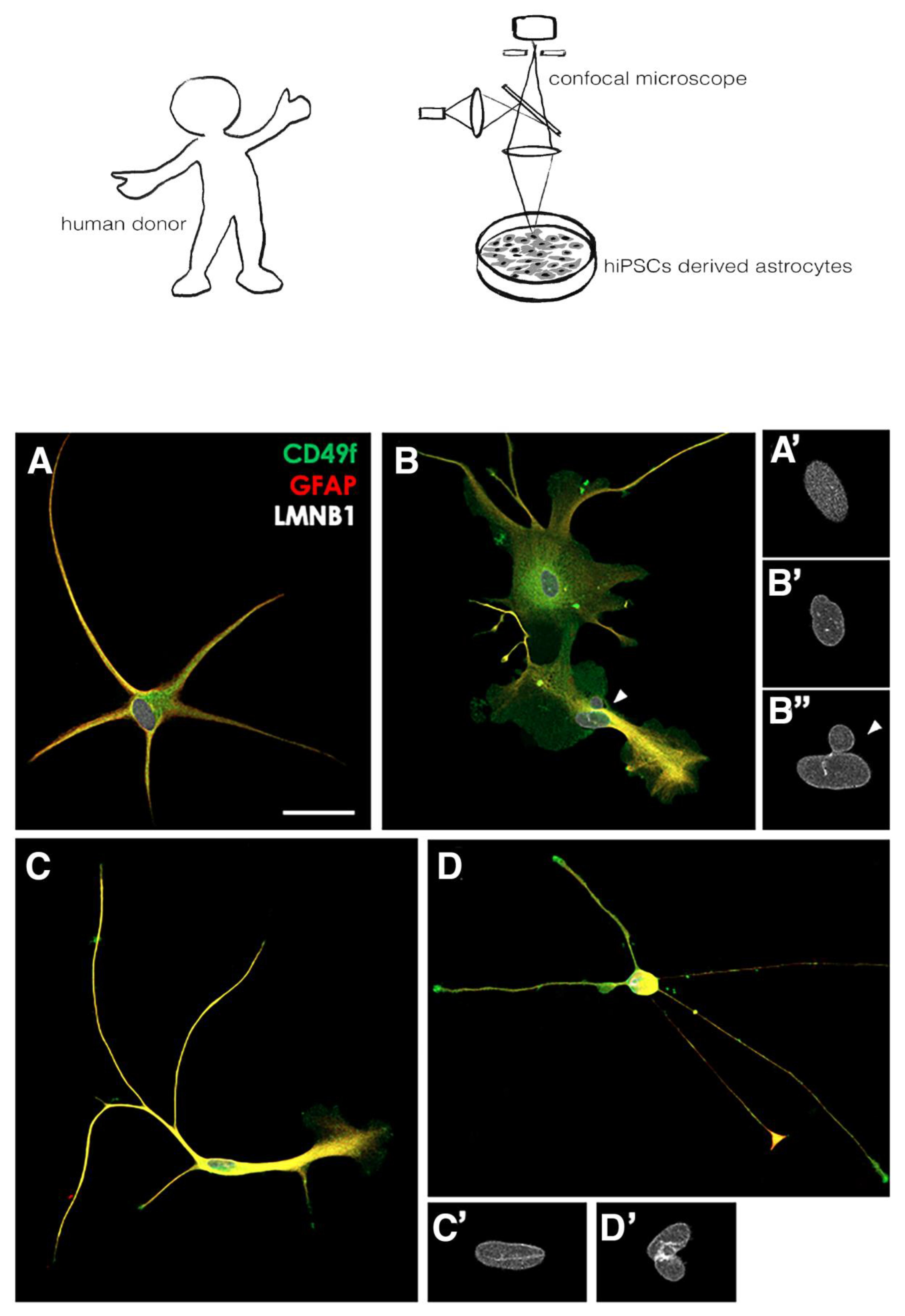
2.1. Human Induced Pluripotent Stem Cell Lines and Cultures

Three hiPSC lines derived from healthy donors were used for the study: ATCC-DYS0100 (C1; derived from the human foreskin fibroblast cell line ATCC SCRC-1041 and reprogrammed using non-integrative Sendai viral transduction; genes: POU5F1, SOX2, KLF4, MYC), GIBCO TMOi001-A (C2; derived from CD34+ progenitors reprogrammed using the non-integrative episomal vector; genes: POU5F1, SOX2, KLF4, MYC, NANOG, LIN28, SV40 T) and WTSIi004-A (C3; derived from male 35–39 years old fibroblasts and reprogrammed using Sendai viral transduction; genes: POU5F1, SOX2, KLF4, MYC). hiPSC lines were cultured in a 37 °C incubator at 5% CO₂ onto vitronectin-coated six-well plates in Essential8 (A1517001; ThermoFisher, Waltham, MA, USA). Lines were passaged every 3–4 days using gentle, non-enzymatic detachment with Versene Solution (15040066; ThermoFisher, Waltham, MA, USA) for 5 min and were replated in Essential8 medium with Revitacell Supplement 1X (A2644501; ThermoFisher, Waltham, MA, USA). All hiPSC lines underwent a periodical rigorous quality check, including a sterility check, mycoplasma testing and a pluripotency check.

2.2. hiPSCs Neural Commitment and Differentiation into Astrocytes

hiPSCs were induced along the neural lineage and differentiated using the protocol published by Douvaras and colleagues [24,25], with minor modifications. Briefly, hiPSCs were enzymatically detached using StemPro Accutase (A1110501; ThermoFisher, Waltham, MA, USA) and plated at 3–4 × 10⁵ cells/well into a vitronectin-coated six-well plate, in Essential8 medium supplemented with Revitacell, for ~16 h, and then kept in culture in Essential8 without Revitacell Supplement, for ~8 h. The medium was then replaced (day in vitro 0, DIV0) with Neural Induction Medium, and the cells were fed daily until DIV7, then with N2 Medium from DIV8 to DIV12. At DIV12, adherent cells were lifted using the StemPro EZPassage Disposable Stem Cell Passaging Tool (23181010; ThermoFisher, Waltham, MA, USA), cultured in suspension into low-attachment dishes, in order to favor sphere formation, and were fed every other day in N2B27 medium until DIV20, then until DIV30 with PDGF Medium (see Table S1 for media composition). On DIV30, spheres were picked and plated onto six-well plates coated with 0.1 mg/mL poly-L-ornithine (PO, P3655; Sigma-Aldrich, Saint Louis, MO, USA), followed by the application of 10 mg/mL laminin (Lam, L2020; Sigma-Aldrich, Saint Louis, MO, USA), at the density of 20 spheres/well. Plated spheres were gently fed with PDGF medium (2/3 media changes) every other day. At DIV70-80, spheres and cells migrated out of the spheres were dissociated with StemPro Accutase for 30 min, passed through a 70 μm cell strainer and sorted for CD49f-positive (CD49f+) cells [26]. CD49f+ sorted astrocytes were then plated at a density of 3000/cm² onto PO/Lam coated μ-Slide 8 well ibiTreat (80826; Ibidi, Gräfelfing, Germany), cultured for three days in PDGF medium, and then fixed with 4% paraformaldehyde (PFA) in 0.1 M sodium phosphate buffer (PB). Samples were washed two times with PBS and stored at 4 °C until immunofluorescence analyses.

2.3. Immunofluorescence and Confocal Analysis

For immunofluorescence reactions, astrocytes were incubated for 24 h at 4 °C in a solution of 0.01 M PBS, pH 7.4, containing 0.5% Triton X-100, 2% normal donkey serum and primary antibodies. Cells were then incubated for 2 h at room temperature, in a solution of 0.01 M PBS, pH 7.4, containing 1% normal donkey serum, 4′,6-diamidino-2-phenylindole dihydrochloride (DAPI; Fluka, Milan, Italy) and appropriate secondary antibodies. Primary and secondary antibodies are reported in Table S2. All the images were acquired with the inverted confocal microscope ZEN LSM800 (Zeiss, Oberkochen, Germany), using 20× magnification in a field of 319.45 × 319.45 µm, zstep = 1 µm. For each technical replicate (n = 3) of each cell line (n = 3), at least 15 astrocytes were analyzed, for a total of 193 astrocytes (C1: n = 55; C2: n = 72; C3: n = 66). Of note, the quantification of GFAP, AQP4, and LMNB1 protein levels throughout immunofluorescence staining required a standardized procedure, in order to avoid technical bias. The same antibody aliquots were used for all the quantification, in order to avoid different specificities, and staining was carried out in parallel on the different samples. Images were acquired using the same confocal parameters, and pixel saturation was avoided, in order to appreciate the entire expression spectrum. Moreover, the images were not post-processed.

2.4. Quantification Analysis

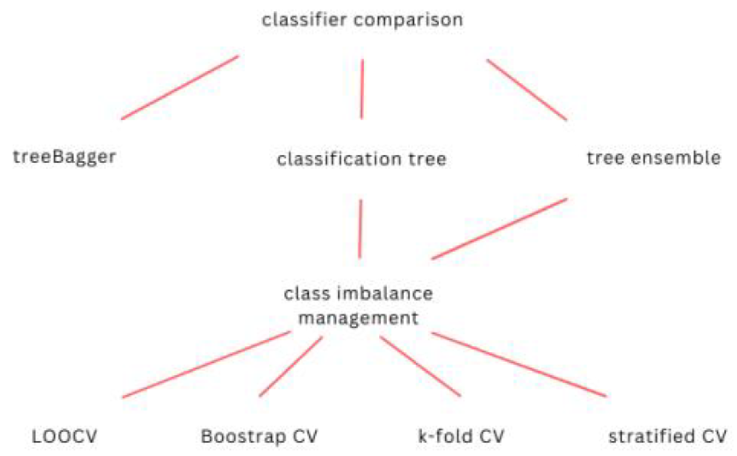
Astrocytes were classified as polygonal or ramified, based on their appearance, and the number of ramifications was counted manually. To segment these cells, we took advantage of Ilastik machine learning software [27]. Briefly, we performed pixel classification to distinguish CD49f labeling from the background, using the Max Intensity ZProjection stack. As an output, we obtained a simple segmentation map containing a 2D mask of CD49f+ astrocytes. This output was finally processed with ImageJ software (available at https://imagej.net/ij/; accessed on 21 March 2023) to measure the area occupied by each segmented cell. Among GFAP+ and/or AQP4+ astrocytes, the integrated density (IntDen) of GFAP and/or AQP4 staining was measured in the central focal plane, exploiting the previously obtained masks. IntDen was normalized on the background around each cell. Nuclei were automatically outlined on the same images with ImageJ software using the DAPI signal, and both the nuclear area and IntDen measurements of LMNB1 protein content were obtained.

2.5. Classification

Classification trees are supervised learning models that work well, both with categorical (classification trees) and quantitative (regression trees) data. The methodology behind classification trees is to recursively split data, based upon the predictors that best distinguish the response variable classes [14,26]. They are computationally efficient and can easily handle continuous and discrete (or mixed) or missing data. They are highly flexible, and naturally uncover complex and nonlinear interactions among the independent variables. Classification trees are also popular because they can easily be combined into learning ensembles. To classify the LMNB1 morphology, we tested several types of classification trees and tree ensembles, in association with different types of cross-validatWeion (CV), in order to assess their performance. Cross-validation (CV) is a method used to evaluate ML models, but it is also strictly intertwined with training; therefore, the choice of CV can influence the accuracy of the model. The simplest cross-validation method consists of splitting the dataset into a training and a test set. This is clearly not a viable method when dealing with small datasets, because it subtracts data for training. Here, we test more sophisticated CV methods such as k-fold CV, bootstrap, leave-one-out CV and stratified CV, in order to optimize the prediction on our sample. We trained three classifiers, a simple tree, an ensemble of bagged trees (TreeBagger) and, finally, an ensemble of boosted classification trees (Tree ensemble), to classify astrocytes into one of five classes: homogeneous, dotted, wrinkled, forming crumples, or forming micronuclei. Alternatively, we also trained the classifiers to classify astrocytes into one of three classes, by merging Classes 1 and 2 together, and 3 and 4 together. The classifiers’ implementation was performed in MATLAB.

To handle class imbalance, we used RUSBoost [16] for the tree ensemble. RUSBoost is an ensemble method that combines the strengths of both random undersampling and the popular boosting algorithm, AdaBoost. By randomly undersampling the majority class and then applying AdaBoost, RUSBoost can balance the class distribution, while also maintaining the strong performance of the boosting algorithm. Additionally, RUSBoost also uses a cost-sensitive approach to weigh the misclassification error of the minority class higher, further addressing the imbalance in the data. Overall, RUSBoost is a powerful technique for handling unbalanced datasets, and has been shown to achieve strong performances in various classification tasks. For the classification tree, we used a cost error matrix. The cost for each class was assigned as the inverse of the frequency. To train the classifiers, we used a set of eight variables: GFAP expression, cell morphology, number or ramifications, cellular area, soma area, nuclear area, normalized intensity of LMNB1, normalized intensity of GFAP, and normalized intensity of AQP4. Since the following variables (normalized intensity of LMNB1, normalized intensity of GFAP, normalized intensity of AQP4, see Table S3) were acquired in different sessions, and their measurement is dependent on acquisition settings, we normalized their values using the z score. Finally, we compared several types of cross-validation: five-fold cross validation, LOOCV, stratified cross-validation and bootstrapping. For bootstrapping, first, we split the sample into training (80%) and testing (20%) datasets, and then resampled both sets with 2500 permutations. Since we were dealing with multiclass classification, the accuracy, sensibility, sensitivity and F1 score were computed for each class, and then averaged weighting for the size of each class was obtained. All analyses were made with Matlab R2022a, The MathWorks, Natick, 2022.

3. Results

3.1. Nuclear Patterns of LMNB1 in Astrocytes

Human lamin B1 is a nuclear protein that is encoded by the LMNB1 gene [22]. Visual inspection of stained astrocytes allowed us to distinguish five morphological nuclear patterns, based on LMNB1 distribution: (0) homogeneous, (1) dotted, (2) wrinkled, (3) forming crumples, (4) forming micronuclei (Figure 1). In our sample we mostly found patterns 0–2. Patterns 3 and 4 were very rare in our samples (

Table 1. Description of LMNB1 morphologies.

LMNB1 Category	N (%)
0	47 (24.35)
1	82 (42.49)
2	48 (24.87)
3	13 (6.47)
4	3 (1.55)

), possibly because these may be linked to cellular dysfunctions, as in case of laminopathies.

A classification based on nuclear expression of LMNB1 has already been performed by Giorgio et al. [22]. They found a higher frequency of homogeneous and dotted morphologies in healthy cells, while morphologies showing crumples were broadly represented in cellular models of autosomal dominant leukodystrophy (ADLD) [22].

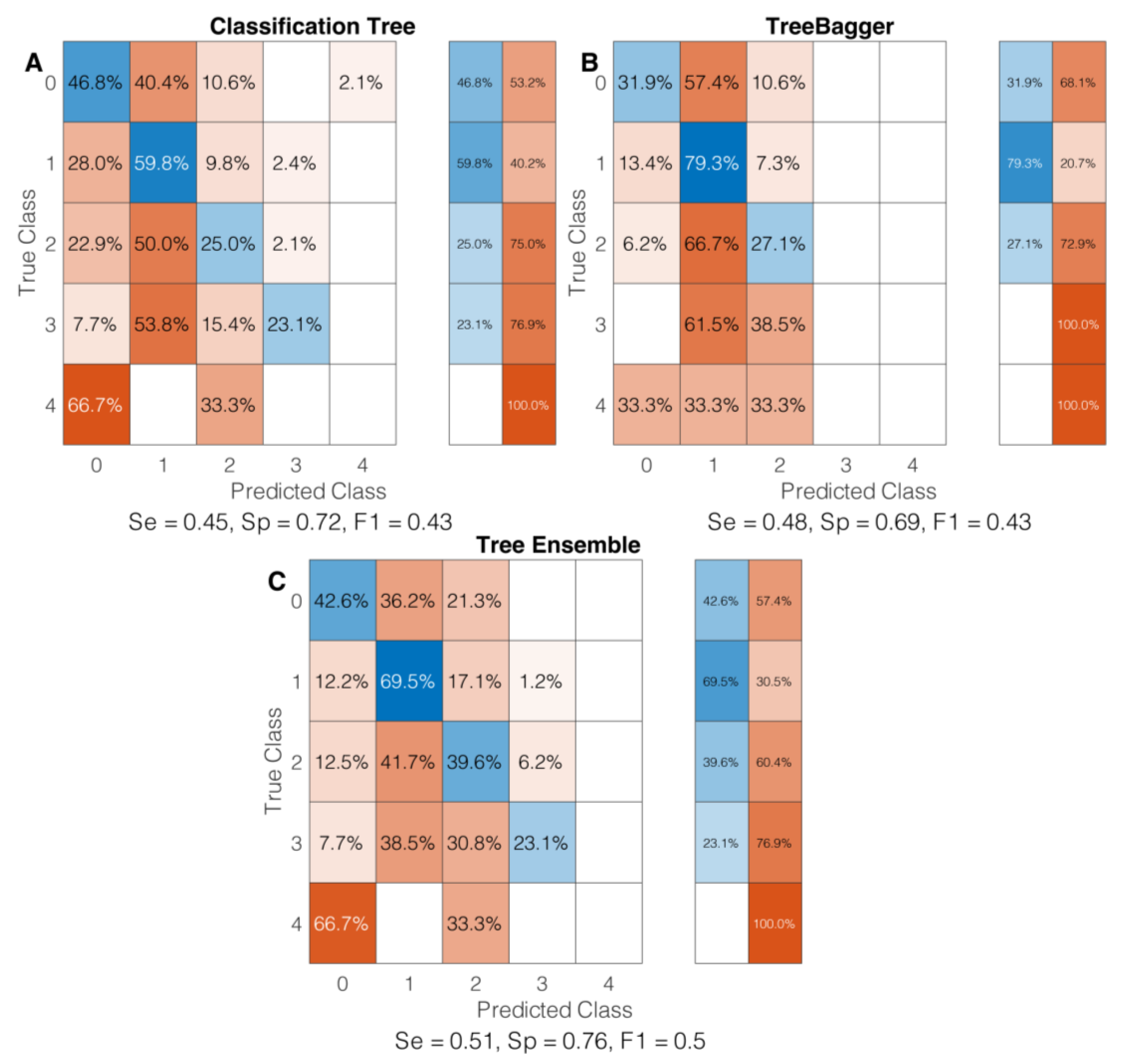
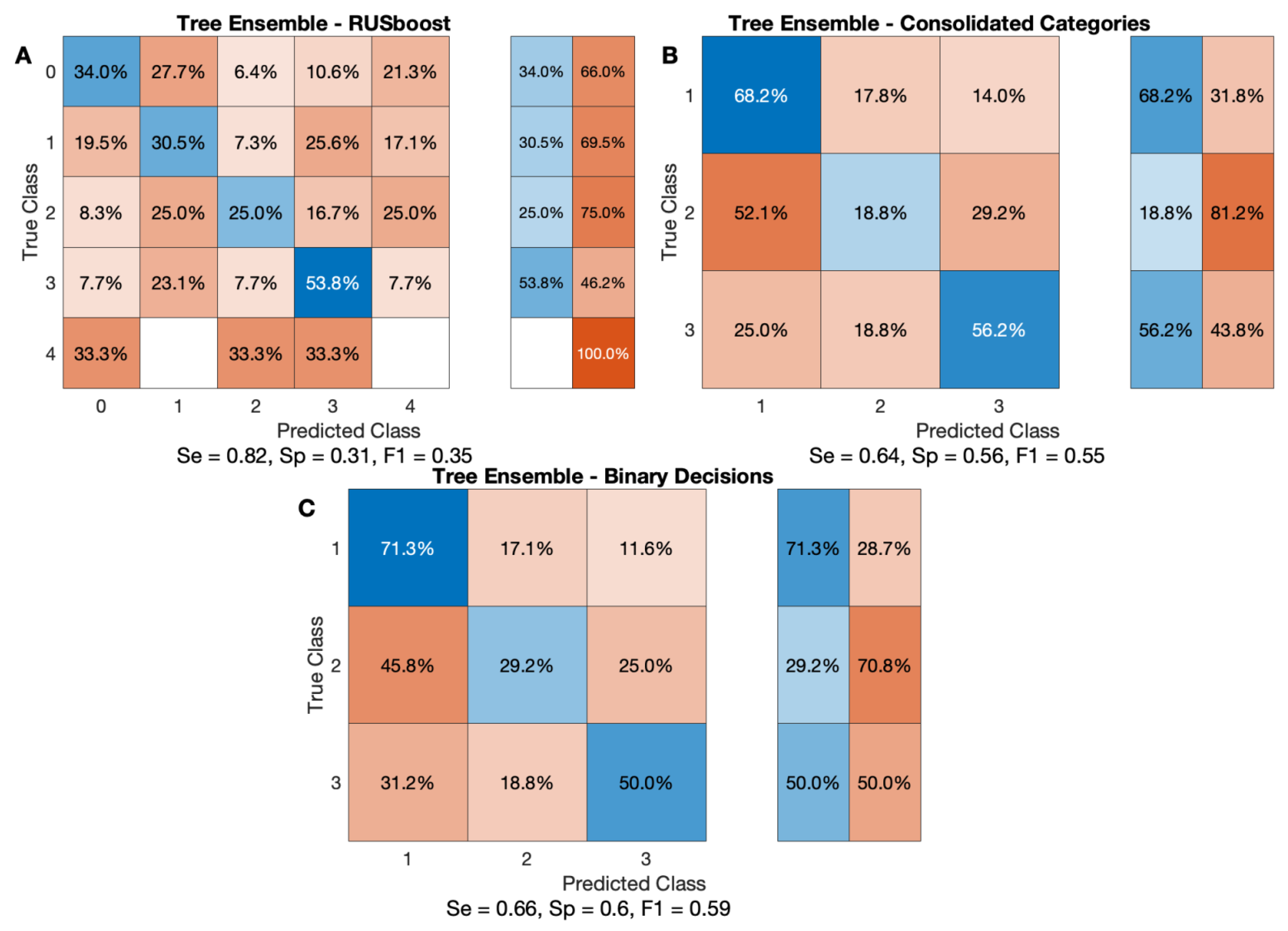
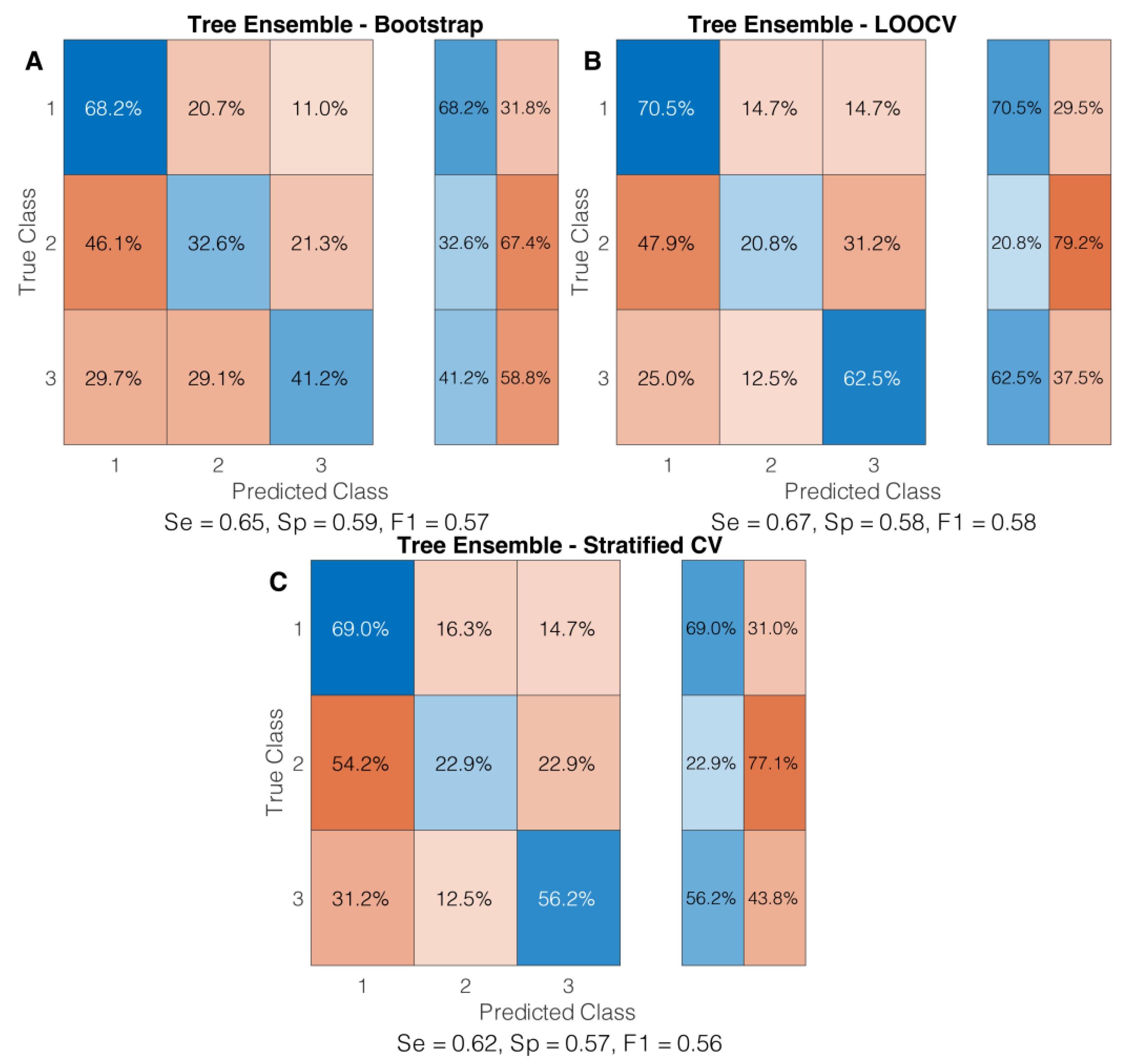
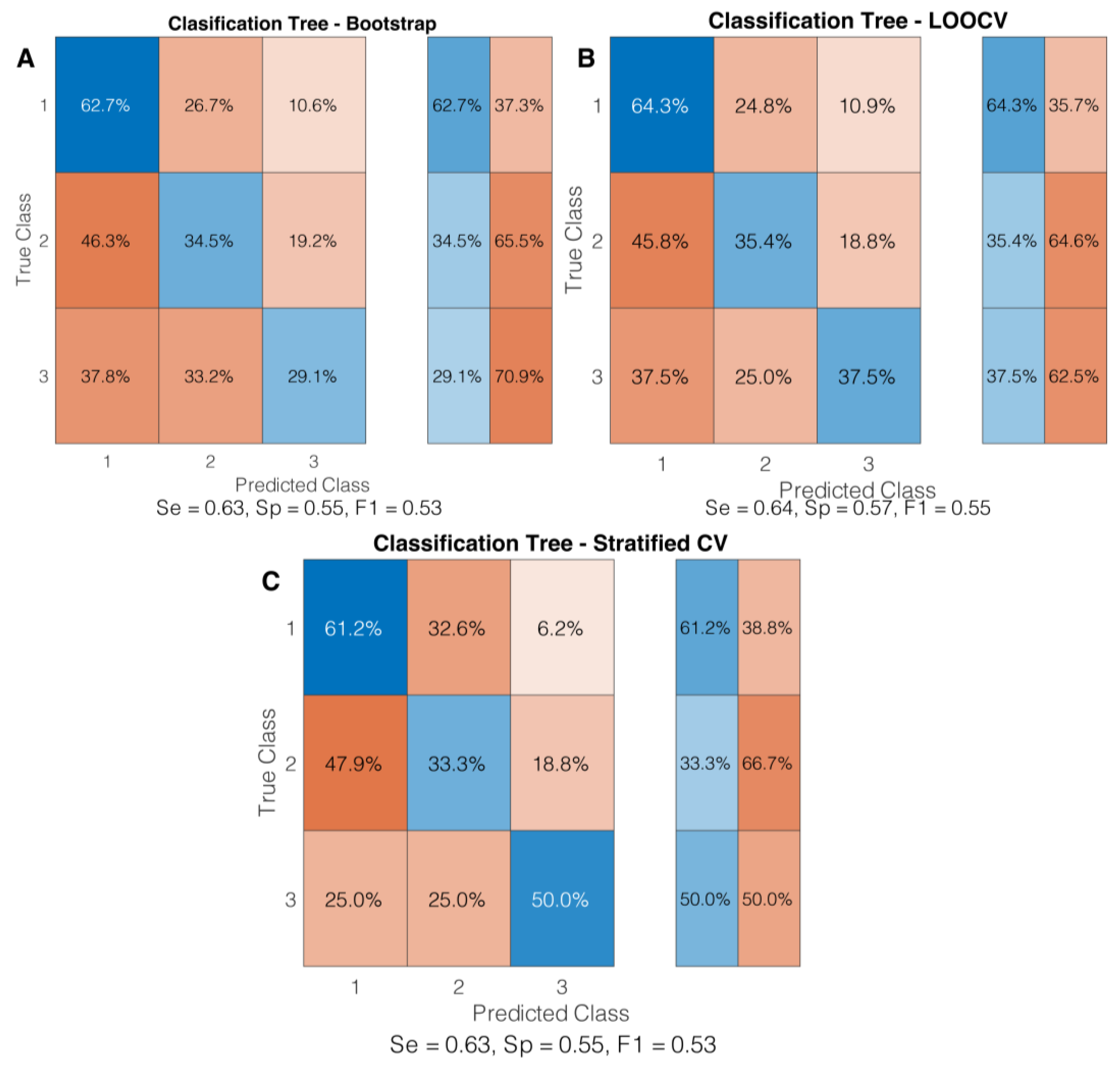
3.2. Classification Algorithm Evaluation

First, we tested the following classifier algorithms on the same subset of data: a simple classification tree, a tree bagger and classification tree ensemble (Figure 2). Tree ensembles have several advantages over a simple tree. They generally lead to improved prediction accuracy and reduced variance. Additionally, they are less prone to overfitting and are more robust to noisy data. They are also able to handle high-dimensional and complex data sets more effectively than a single decision tree. We optimized the hyperparameters using Bayesian optimization, in order to optimize the cross-validation loss of the classifier. For the ensemble algorithms, the optimization function searched for the maximum number of splits among integers log-scaled in the range [1, n observations − 1] = 8, the number of learners among integers log-scaled in the range [10, 500] = 12, the learning rate among real values log-scaled in the range [0.001, 1] = 1 (the learning rate is a regularization parameter that shrinks the contribution of each new tree added to the ensemble; the slower the learning rate, the slower the model learns, becoming more robust) and, finally, the number of predictors to sample among integers in the range [1, number of the predictors] = 8. For the simple classification tree, the optimized parameters comprised the maximum number of splits among integers, log-scaled in the range [1, n observations − 1] = 5, as well as the split criterion along Gini’s index, Twoing rule and Maximum deviance reductions = deviance reduction.

3.3. Cross-Validation Techniques

We used 5-fold cross-validation (CV) to validate the models. We created a confusion chart to compare the predicted outcomes with the observed ones. Figure 3A–C show the confusion charts for each classifier. Rows represent the true classes, and columns represent the predicted classes of the five LMNB1 morphologies (0, 1, 2, 3, 4). The diagonal squares show the intersection of true class and predicted class, e.g., the correct predictions. The off-diagonal squares show the incorrect predictions. White squares indicate zeros.

The classification tree (Figure 3A) only worked well for Classes 0 and 1 and performed sub optimally for all other classes. We calculated the sensitivity, specificity and F1 score (see Materials and Methods). Although very similar, the tree ensemble yields the best results, therefore, we chose this classifier for further analysis.

A closer look at the data shows that the five classes are highly unbalanced (Table 1) with Class 1 being the most represented, followed by Classes 0 and 2. Classes 3 and 4 are the sparsest. This explains why all the classifiers consistently performed poorly for Classes 3 and 4. To handle this class imbalance, we used RUSBoost, an algorithm that uses a combination of random under-sampling (RUS), as well as AdaBoost, in order to better predict the less represented classes. Figure 4A shows the performance of the classification ensemble using RUSBoost. Although the use of RUSBoost reduces the F1 score (compare Figure 3C with Figure 4A), it largely improves the prediction for Class 3, one of the least-represented ones (Figure 4A).

Since we wanted to obtain a more balanced accuracy across classes, we used RUSBoost with all the following models presented in this paper. In order to reduce class imbalance, we merged the five original categories into three larger classes, according to morphological similarities described by Giorgio et al. [22]: Class 1: formed by former Categories 0 and 1; Class 2: formed by former Category 2; Class 3: formed by former Category 3 and 4. We applied the same model to these three larger classes; the results are shown in Figure 5B. The F1 score increases sharply, and the model performs well for Classes 1 and 3, but not for Class 2.

All the models in this figure were cross-validated with five-fold cross-validation. Usually, machine learning algorithms are optimized for binary decisions, rather than multiple class decisions. However, for multiclass problems, we decided to test a technique called “one vs. all” (also known as “one vs. the rest”), where a separate binary classifier is trained for each class to predict whether an example belongs to that class or not. This can lead to improved performance compared to using a single multiclass classifier [28]. One vs. all (also known as “one vs. the rest”) is a technique used for multiclass classification problems, where a separate binary classifier is trained for each class to predict whether an example belongs to that class or not. The class that is predicted by the classifier with the highest confidence score is the final prediction. This method is based on the idea that a good classifier for a problem with multiple classes should be able to separate each class from the rest of the classes. By training a separate classifier for each class, the one vs. all method attempts to achieve this goal. To assign the decision to one class, we determined the decision that had the highest score, which is a measure of the probability of an observation belonging to a particular class. It can be used to decide the class of an observation based on a threshold. (Figure 4C). Next, we tried to optimize cross-validation (CV). CV is a key step in machine learning. It is a method to evaluate ML models by correcting for overfitting, in order to improve the model’s ability to generalize. It also estimates the goodness of a model. The most used is k-fold CV, which we used for all models in Figure 3 and Figure 4. However k-fold CV may not be the best for small samples, since some classes may be absent from one or more folds. Therefore, we tested bootstrapping, leave-one-out (LOOCV) and stratified CV. Bootstrapping is a method used to simulate new samples from a single data set, by performing resampling with replacement. LOOCV uses a single observation as a validation set and all the remaining data as a training set. Therefore, LOOCV creates as many models as the sample size (193 in our case) and tests them the same number of times. Stratified CV ensures that all the outcome classes have an even proportion of outcome classes, so that that CV’s results are a closer approximation of the real prediction error. We obtained the best predictions with LOOCV (Figure 5B). At the beginning of the study (Figure 3), we showed that the tree ensemble performs better for our data than the other models. However, it is possible that, with different cross-validations, the performance of other models improves too. Therefore, we tested bootstrapping, LOOCV and stratified CV also on the classification tree (Figure 6). To address class imbalance and reduce prediction bias, we implemented a cost-sensitive error function that applies a higher penalty for errors in the over-represented classes. Specifically, the cost error was calculated as the reciprocal of the class frequency.

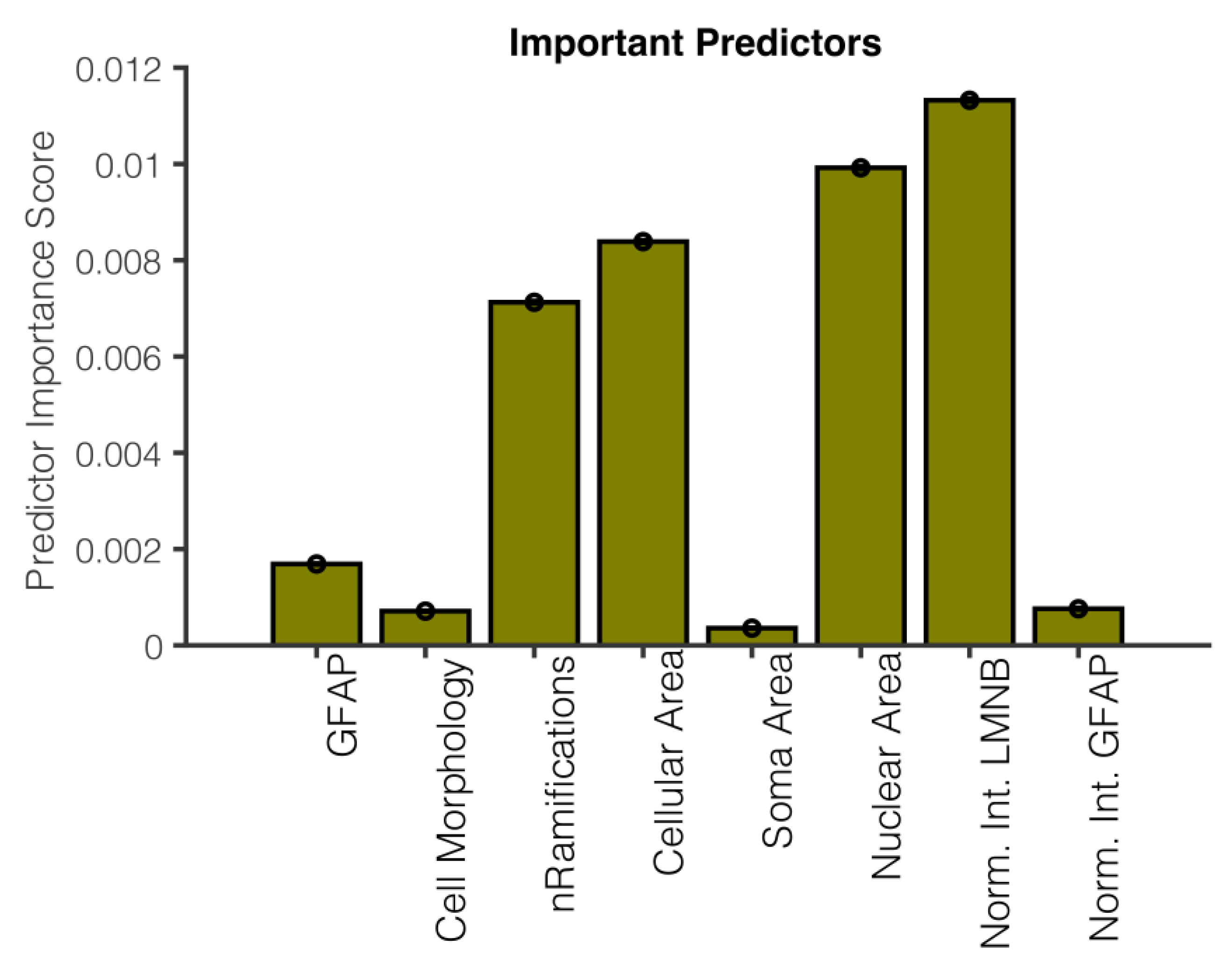
3.4. Important Predictors

Finally, we quantified the importance of the predictors. Figure 7 shows that the three most important variables are the following: the normalized intensity of LMNB1, nuclear area, cellular area, and number of ramifications. The important predictors were calculated by quantifying how crucial each predictor is in a decision tree, by adding up the variations in risk at each node caused by splits on every predictor, and then dividing that sum by the total number of branching nodes. The alteration in the risk at a node is calculated by subtracting the risk of the parent node from the total risk of its child nodes. To illustrate, when a tree separates a parent node (e.g., Node 1) into two child nodes (e.g., Nodes 2 and 3), the function increases the importance of the predictor used for that split by the difference in risk between the parent node and child nodes [28].

4. Discussion

Machine learning is widely used in neurophysiology and integrative neuroscience to decode single/multi-unit recordings [29,30,31,32] or voxel pattern activations from fMRI [33], in neural prosthetics [34], and in many other applications. However, ML is still not commonly used for histological data analysis. Here we applied machine learning to classify in vitro cultivated astrocytes according to their nuclear expression of LMNB1. We used eight morphological features to predict five nuclear morphologies of LMNB1 expression. We trained several classifiers to this task and showed that tree ensembles can classify astrocyte morphology at rates better than chance. This is a step towards the automation of histologic data analysis, which is important, considering the development of techniques for faster anatomical data production, such as CLARITY [35] and PACT [36] that do not require time-consuming slicing of the brain.

Our results show that a single classification tree predicts less accurately than tree ensembles. This is consistent with [37], who showed that an ensemble of weak learners can predict highly unbalanced data more accurately. Surprisingly, we found that the tree ensemble performs better than the tree bagger. Tree bagger is an algorithm that works very similarly to the random forest, which is considered the benchmark for this kind of analyses [38]. This is probably because the tree ensemble relies on a boosting algorithm, where individual trees work in series and each tree is presented with the whole training sample, whereas the tree bagger is a bagging algorithm, where several trees work in parallel and each of them is trained on a subset of the samples, so that every tree is trained on an even smaller sample than the initial one.

We also showed that the best results are obtained using RUSBoost instead of ADABoost, and by combining LMNB1 categories by morpho-functional similarities. Finally, we tested several types of cross validation. We obtained the best results with LOOCV, however bootstrapping yielded more balanced results, in that it also gave good results for Class 3, the least represented one. LOOCV and bootstrapping are the most computationally intensive and time-consuming CVs, however, they offer broader exposure to all categories during the training phase [39].

Finally, we estimated the important predictors: the normalized intensity of LMNB1, nuclear area, cellular area, and the number of ramifications. Although it is not surprising that the intensity of expression of the LMNB1 protein may be related to the way in which it is expressed in the nucleus, we are not aware of any previous research or evidence that has specifically examined this relationship. This suggests that this may be a new or novel finding, and further research may be needed to confirm and explore this potential correlation. On the other hand, the other three important predictors are a novel finding, and open new perspectives on the mechanism of action of LMNB1 and its expression. None of the predictors considered were able to predict the membership class on their own as accurately as when they were combined with the other features. This suggests that the relationship between these predictors and the LMNB1 class is likely to be complex, and may not follow a simple, linear pattern. Together, our analyses show new perspectives regarding the understanding of the relationships between cellular features that are difficult to study with simpler statistical tools. In future work, it would be important to validate the results obtained from our small data sample on a larger and more diverse dataset. Moreover, exploring other machine learning algorithms or techniques, could potentially yield even better results. Finally, it would be interesting to investigate the biological significance of the identified predictors and their potential role in astrocyte function and physiology.

5. Conclusions

In conclusion, we were able to classify astrocytes, from a small data sample, into classes based on LMNB1 expression patterns. Tree ensembles outperformed single classification trees and tree bagger in this task. The best results were obtained using leave-one-out cross-validation (LOOCV) or bootstrap. The normalized intensity of LMNB1, nuclear area, cellular area, and the number of ramifications were found to be important predictors in the classification process. These results offer new hints into the mechanisms of action and expression of LMNB1 and show the potential for the use of machine learning in finding associations between unexpected cell features that look uncorrelated at first examination. Our findings suggest that machine learning can be a powerful tool for uncovering hidden associations between seemingly unrelated cell features, shedding light on the complex mechanisms of action and expression of LMNB1 in astrocytes. These results offer valuable insights into the biology of astrocytes, and open new avenues for further investigations into the role of LMNB1 in regulating their functions.

References

1. Mittal, U.; Chawla, P.; Tiwari, R. EnsembleNet: A Hybrid Approach for Vehicle Detection and Estimation of Traffic Density Based on Faster R-CNN and YOLO Models. Neural Comput. Appl. 2022, 35, 4755–4774. [Google Scholar] [CrossRef]
2. Formosa, N.; Quddus, M.; Ison, S.; Abdel-Aty, M.; Yuan, J. Predicting Real-Time Traffic Conflicts Using Deep Learning. Accid. Anal. Prev. 2020, 136, 105429. [Google Scholar] [CrossRef] [PubMed]
3. Nam, D.; Lavanya, R.; Jayakrishnan, R.; Yang, I.; Jeon, W.H. A Deep Learning Approach for Estimating Traffic Density Using Data Obtained from Connected and Autonomous Probes. Sensors 2020, 20, 4824. [Google Scholar] [CrossRef] [PubMed]
4. Hashad, K.; Gu, J.; Yang, B.; Rong, M.; Chen, E.; Ma, X.; Zhang, K.M. Designing Roadside Green Infrastructure to Mitigate Traffic-Related Air Pollution Using Machine Learning. Sci. Total. Environ. 2021, 773, 144760. [Google Scholar] [CrossRef] [PubMed]
5. Verma, P.; Tiwari, R.; Hong, W.-C.; Upadhyay, S.; Yeh, Y.-H. FETCH: A Deep Learning-Based Fog Computing and IoT Integrated Environment for Healthcare Monitoring and Diagnosis. IEEE Access 2022, 10, 12548–12563. [Google Scholar] [CrossRef]
6. Rauschert, S.; Raubenheimer, K.; Melton, P.E.; Huang, R.C. Machine Learning and Clinical Epigenetics: A Review of Challenges for Diagnosis and Classification. Clin. Epigenet. 2020, 12, 51. [Google Scholar] [CrossRef] [Green Version]
7. Yuan, J.; Ran, X.; Liu, K.; Yao, C.; Yao, Y.; Wu, H.; Liu, Q. Machine Learning Applications on Neuroimaging for Diagnosis and Prognosis of Epilepsy: A Review. J. Neurosci. Methods 2022, 368, 109441. [Google Scholar] [CrossRef]
8. Kabade, V.; Hooda, R.; Raj, C.; Awan, Z.; Young, A.S.; Welgampola, M.S.; Prasad, M. Machine Learning Techniques for Differential Diagnosis of Vertigo and Dizziness: A Review. Sensors 2021, 21, 7565. [Google Scholar] [CrossRef]
9. Bathla, G.; Singh, P.; Singh, R.K.; Cambria, E.; Tiwari, R. Intelligent Fake Reviews Detection Based on Aspect Extraction and Analysis Using Deep Learning. Neural Comput. Appl. 2022, 34, 20213–20229. [Google Scholar] [CrossRef]
10. Nagaraju, M.; Chawla, P.; Upadhyay, S.; Tiwari, R. Convolution Network Model Based Leaf Disease Detection Using Augmentation Techniques. Expert. Syst. 2022, 39, e12885. [Google Scholar] [CrossRef]
11. Kokol, P.; Kokol, M.; Zagoranski, S. Machine Learning on Small Size Samples: A Synthetic Knowledge Synthesis. Sci. Prog. 2022, 105, 368504211029777. [Google Scholar] [CrossRef] [PubMed]
12. Vu, M.-A.T.; Adalı, T.; Ba, D.; Buzsáki, G.; Carlson, D.; Heller, K.; Liston, C.; Rudin, C.; Sohal, V.S.; Widge, A.S.; et al. A Shared Vision for Machine Learning in Neuroscience. J. Neurosci. 2018, 38, 1601–1607. [Google Scholar] [CrossRef] [PubMed] [Green Version]
13. Vabalas, A.; Gowen, E.; Poliakoff, E.; Casson, A.J. Machine Learning Algorithm Validation with a Limited Sample Size. PLoS ONE 2019, 14, e0224365. [Google Scholar] [CrossRef]
14. Breiman, L.; Friedman, J.H.; Olshen, R.A.; Stone, C.J. Classification and Regression Trees, 1st ed.; Routledge: Oxford, UK, 2017; ISBN 978-1-315-13947-0. [Google Scholar]
15. Das, B. SMOTEBoost 2022. Available online: https://it.mathworks.com/matlabcentral/fileexchange/37311-smoteboost (accessed on 21 March 2023).
16. Das, B. RUSBoost 2022. Available online: https://it.mathworks.com/matlabcentral/fileexchange/37315-rusboost (accessed on 21 March 2023).
17. Shimi, T.; Butin-Israeli, V.; Adam, S.A.; Hamanaka, R.B.; Goldman, A.E.; Lucas, C.A.; Shumaker, D.K.; Kosak, S.T.; Chandel, N.S.; Goldman, R.D. The Role of Nuclear Lamin B1 in Cell Proliferation and Senescence. Genes. Dev. 2011, 25, 2579–2593. [Google Scholar] [CrossRef] [Green Version]
18. Camps, J.; Erdos, M.R.; Ried, T. The Role of Lamin B1 for the Maintenance of Nuclear Structure and Function. Nucleus 2015, 6, 8–14. [Google Scholar] [CrossRef] [Green Version]
19. Shah, P.P.; Donahue, G.; Otte, G.L.; Capell, B.C.; Nelson, D.M.; Cao, K.; Aggarwala, V.; Cruickshanks, H.A.; Rai, T.S.; McBryan, T.; et al. Lamin B1 Depletion in Senescent Cells Triggers Large-Scale Changes in Gene Expression and the Chromatin Landscape. Genes. Dev. 2013, 27, 1787–1799. [Google Scholar] [CrossRef] [Green Version]
20. Bedrosian, T.A.; Houtman, J.; Eguiguren, J.S.; Ghassemzadeh, S.; Rund, N.; Novaresi, N.M.; Hu, L.; Parylak, S.L.; Denli, A.M.; Randolph-Moore, L.; et al. Lamin B1 Decline Underlies Age-related Loss of Adult Hippocampal Neurogenesis. EMBO J. 2021, 40, e105819. [Google Scholar] [CrossRef]
21. Padiath, Q.S.; Saigoh, K.; Schiffmann, R.; Asahara, H.; Yamada, T.; Koeppen, A.; Hogan, K.; Ptáček, L.J.; Fu, Y.-H. Lamin B1 Duplications Cause Autosomal Dominant Leukodystrophy. Nat. Genet. 2006, 38, 1114–1123. [Google Scholar] [CrossRef] [PubMed]
22. Giorgio, E.; Lorenzati, M.; Rivetti di Val Cervo, P.; Brussino, A.; Cernigoj, M.; Della Sala, E.; Bartoletti Stella, A.; Ferrero, M.; Caiazzo, M.; Capellari, S.; et al. Allele-Specific Silencing as Treatment for Gene Duplication Disorders: Proof-of-Principle in Autosomal Dominant Leukodystrophy. Brain 2019, 142, 1905–1920. [Google Scholar] [CrossRef] [Green Version]
23. Hasel, P.; Liddelow, S.A. Astrocytes. Curr. Biol. 2021, 31, R326–R327. [Google Scholar] [CrossRef]
24. Douvaras, P.; Fossati, V. Generation and Isolation of Oligodendrocyte Progenitor Cells from Human Pluripotent Stem Cells. Nat. Protoc. 2015, 10, 1143–1154. [Google Scholar] [CrossRef] [PubMed]
25. Douvaras, P.; Wang, J.; Zimmer, M.; Hanchuk, S.; O’Bara, M.A.; Sadiq, S.; Sim, F.J.; Goldman, J.; Fossati, V. Efficient Generation of Myelinating Oligodendrocytes from Primary Progressive Multiple Sclerosis Patients by Induced Pluripotent Stem Cells. Stem Cell. Rep. 2014, 3, 250–259. [Google Scholar] [CrossRef] [PubMed] [Green Version]
26. Barbar, L.; Jain, T.; Zimmer, M.; Kruglikov, I.; Sadick, J.S.; Wang, M.; Kalpana, K.; Rose, I.V.L.; Burstein, S.R.; Rusielewicz, T.; et al. CD49f Is a Novel Marker of Functional and Reactive Human IPSC-Derived Astrocytes. Neuron 2020, 107, 436–453.e12. [Google Scholar] [CrossRef]
27. Berg, S.; Kutra, D.; Kroeger, T.; Straehle, C.N.; Kausler, B.X.; Haubold, C.; Schiegg, M.; Ales, J.; Beier, T.; Rudy, M.; et al. Ilastik: Interactive machine learning for (bio)image analysis. Nat. Methods 2019, 16, 1226–1232. [Google Scholar] [CrossRef]
28. Breiman, L. Random Forests. Mach. Learn. 2001, 45, 5–32. [Google Scholar] [CrossRef] [Green Version]
29. Merk, T.; Peterson, V.; Köhler, R.; Haufe, S.; Richardson, R.M.; Neumann, W.-J. Machine Learning Based Brain Signal Decoding for Intelligent Adaptive Deep Brain Stimulation. Exp. Neurol. 2022, 351, 113993. [Google Scholar] [CrossRef] [PubMed]
30. Vyas, S.; Golub, M.D.; Sussillo, D.; Shenoy, K.V. Computation Through Neural Population Dynamics. Annu. Rev. Neurosci. 2020, 43, 249–275. [Google Scholar] [CrossRef]
31. Thomas, A.W.; Ré, C.; Poldrack, R.A. Interpreting Mental State Decoding with Deep Learning Models. Trends Cogn. Sci. 2022, 26, 972–986. [Google Scholar] [CrossRef]
32. Odegaard, B.; Grimaldi, P.; Cho, S.H.; Peters, M.A.K.; Lau, H.; Basso, M.A. Superior Colliculus Neuronal Ensemble Activity Signals Optimal Rather than Subjective Confidence. Proc. Natl. Acad. Sci. USA 2018, 115, E1588–E1597. [Google Scholar] [CrossRef] [Green Version]
33. Boutet, A.; Madhavan, R.; Elias, G.J.B.; Joel, S.E.; Gramer, R.; Ranjan, M.; Paramanandam, V.; Xu, D.; Germann, J.; Loh, A.; et al. Predicting Optimal Deep Brain Stimulation Parameters for Parkinson’s Disease Using Functional MRI and Machine Learning. Nat. Commun. 2021, 12, 3043. [Google Scholar] [CrossRef]
34. Li, Y.; Qi, Y.; Wang, Y.; Wang, Y.; Xu, K.; Pan, G. Robust Neural Decoding by Kernel Regression with Siamese Representation Learning. J. Neural Eng. 2021, 18, 056062. [Google Scholar] [CrossRef] [PubMed]
35. Chung, K.; Deisseroth, K. CLARITY for Mapping the Nervous System. Nat. Methods 2013, 10, 508–513. [Google Scholar] [CrossRef] [PubMed]
36. Yang, B.; Treweek, J.B.; Kulkarni, R.P.; Deverman, B.E.; Chen, C.-K.; Lubeck, E.; Shah, S.; Cai, L.; Gradinaru, V. Single-Cell Phenotyping within Transparent Intact Tissue through Whole-Body Clearing. Cell 2014, 158, 945–958. [Google Scholar] [CrossRef] [PubMed] [Green Version]
37. Vong, C.-M.; Du, J. Accurate and Efficient Sequential Ensemble Learning for Highly Imbalanced Multi-Class Data. Neural Netw. 2020, 128, 268–278. [Google Scholar] [CrossRef] [PubMed]
38. Tin Kam Ho The Random Subspace Method for Constructing Decision Forests. IEEE Trans. Pattern Anal. Mach. Intell. 1998, 20, 832–844. [CrossRef] [Green Version]
39. Efron, B.; Tibshirani, R.J. An Introduction to the Bootstrap; Chapman and Hall/CRC: Boca Raton, FL, USA, 1994; ISBN 978-0-429-24659-3. [Google Scholar]
Figure 1. hiPSC-derived astrocytes display different morphological nuclear LMNB1-related patterns. Human pluripotent stem cells derived from healthy donors were differentiated to neural progenitors, expanded as spheres, further matured into authentic astrocytes (see Section 2), and analyzed by confocal microscopy (A). During this maturation step, they acquired typical astroglial markers (GFAP, CD49f) and morphologies (BD). Astrocyte nuclei were classified into 5 categories, corresponding to distinct nuclear morphologies based on the LMNB1 staining pattern: homogeneous (A’, with no sign of LMNB1 accumulation), dotted (B’, with dots of LMNB1 accumulations), wrinkled (C’, with stripes of LMNB1 accumulations), forming crumples, (D’) or forming micronuclei (B’’). Magnification in A’, B’, B’’, C’ and D’ shows LMNB1 staining details. GFAP, Glial Fibrillary Acid Protein; LMNB1, Lamin B1. Scale bar: 50 µm.
Applsci 13 04289 g001
Figure 2. Flow chart of the experimental design. To classify astrocytes’ morphology, we compared three classifier algorithms; we used methods to address class imbalance like RUSBoost and cost sensitive error functions. We also used four types of cross-validation.
Applsci 13 04289 g002
Figure 3. Confusion charts of three learners: classification tree (A), Treebagger (B), tree ensemble (C). Se = sensitivity, Sp = specificity, F1 = F score. All the models in this figure were cross-validated with 5-fold cross-validation.
Applsci 13 04289 g003
Figure 4. Confusion charts for (A) prediction of a tree ensemble on five categories using RUSBoost. (B) Prediction of the same tree ensemble for three consolidated categories. (C) Prediction of the binary decision model.
Applsci 13 04289 g004
Figure 5. Shows three confusion matrices for the tree ensemble with different types of cross-validation. (A) Shows bootstrap CV, (B) shows leave-one-out CV and (C) shows stratified CV.
Applsci 13 04289 g005
Figure 6. Confusion matrices for tree ensemble classification trees with different types of cross-validation. (A) Shows bootstrap CV, (B) shows leave-one-out CV and (C) shows stratified CV.
Applsci 13 04289 g006
Figure 7. Bar graph showing the important predictors of a tree ensemble model cross-validated with LOOCV, Figure 5B. The x-axis represents the predictor variables, and the y-axis shows the importance score assigned to each predictor by the model.
Applsci 13 04289 g007