Applicability of Sun’s Empirical Relations for Non-Uniform Sediment in Jiaojiang Estuaries, Zhejiang, China

Abstract

The numerical simulation of non-uniform sediment transport under tidal flow in estuaries is a complicated, yet important, issue in Zhejiang estuaries. In this paper, a depth-averaged two-dimensional (2D) mathematical model for non-uniform sediment transport in estuaries is established and applied in Zhejiang tidal estuaries based on several newly derived formulas by Zhlin Sun et al. The model is validated using data from several experiments, including an aggradation test and an erosion test. Good performance in the tests indicates that the present model can simulate aggradation and erosion processes of non-uniform sediment. The model is also verified by observational data from the Jiaojiang estuary, and calculations agree well with measurements. The model is thus adaptable to simulating flow and non-uniform sediment transport in tidal estuaries.

1. Introduction

Compared with physical models of sediment transport, numerical models have several advantages, such as low running costs, fast simulation speed, and convenient parameter adjustment. Thus, numerical models have wide applications in the planning, design, and assessment of estuarine and coastal engineering [1,2,3,4,5].

Previous efforts to model sediment transport have conducted lots of work based on non-uniform sediment that exists in natural rivers and coastal waters [2]. Research showed that models considering multiple sediment classes appeared to be better suited to simulate suspended sediment transport in the Tagus estuary than models using a single grain size [6]. In the numerical experiments, the computed results improved significantly when they used non-uniform sediment transport formulas or a modified approach [7]. Research also demonstrated that a model considering non-uniform sediment transport yielded the results that were consistent with measurements, while a model that only considered uniform sediment under-predicted or over-predicted the sediment transport rates [8,9]. It has been found that dividing sediments into a number of classes and separately simulating each sediment size class improved predictions [10]. In contrast, they found that the traditional approach of adjusting the sediment in a multi-disperse mixture to consider all particle sizes does not accurately predict the distribution of volumetric sediment concentrations. As a result, models using non-uniform sediment parameters show better simulation reliability than uniform sediment methods. Zhejiang, where the estuary of one of the world’s biggest river lies, is one of the most densely distributed areas of estuaries in China. The flow structure and sediment transport are complicated under the combined influence of natural and anthropic factors. Quantification of sediment transport in tidal estuaries is essential to support both theoretical, as well as numerical modelling, of tidal estuarine morphodynamic evolution. Obtaining high-resolution data of sediment transport is hard. Both physical modelling and numerical simulation methods have been employed to investigate the sediment transport problem in estuaries. Novak et al. [11] elaborated on the theory and design of different river engineering models, including estuarine and coastal conditions. Davinroy et al. [12] proposed a small-scale riverine model, and Maynord et al. [13] reviewed its applicability.

Flow in estuary is subject to the combined effect of tide and residual runoff, and sediment flux comes in both directions, thus creating a complex dynamic environment. Compared with inland rivers, the sediment transport in tidal estuaries is more complex and therefore more difficult to simulate [14,15,16]. The estuarine zone is where the land and sea interact. Various physical processes, such as current, waves, and sediments, are coupled and add to computation complexity. In recent years, a few non-uniform sediment numerical models have been proposed in the literature. Lu et al. [17] established a two-dimensional non-uniform sediment transport model for the Oujiang estuary and Wenzhou Bay by using the sediment transport capacity formula for uniform sediment. Wu et al. [18,19] developed two models for non-uniform sediment transport in channels by considering hiding-exposure effects among different size classes. Fang et al. [20,21] proposed a one-dimensional and a three-dimensional model for non-uniform sediment transport in rivers by using a formula for sediment transport capacity that did not consider the interaction between fractions. Hung et al. [22] described a two-dimensional model for non-uniform sediment transport in alluvial channels by using empirical values for the critical bed-shear stresses for erosion and deposition. Xiao et al. [23] presented a two-dimensional model for mixed-grain size sediment transport by considering grain-sorting effects in non-uniform sediment. Hu et al. [24] proposed a one-dimensional model using the surface-based formulation (SBF), which uses sediment exchange flux in estimating the sediment fraction instead of the traditional active layer formulation (ALF). Qian et al. [25] presented a one-dimensional well balanced model to simulate flows and non-capacity transport of non-uniform sediment in alluvial rivers. Most of the present models for non-uniform sediment transport use formulas for uniform sediment for calculations involving the various particle size fractions of non-uniform sediment or use empirical values for key parameters. Besides, most sediment formulas were not optimized for the Zhejiang area and did not show good compatibility. To better describe non-uniform sediment transport, Sun [26,27,28,29,30,31,32] deduced the probability of the fractional incipient motion for non-uniform sediment. This allowed the critical bed-shear stress for erosion and deposition of non-uniform sediment to be calculated [31,32]. The erosion coefficients for cohesive non-uniform sediment are suggested [31]. In addition, Sun [26] derived a quasi-theoretical formula for the settling velocity of any particle size in various passing-flow states.

In this paper, Sun’s theories for non-uniform sediment transport are used to develop a depth-averaged two-dimensional mathematical model in estuaries. We encode Sun’s formulas about non-uniform sediment into the numerical model and aim to further verify Sun’s theories for non-uniform sediment transport using numerical examples and practical applications. The resulting model can be applied to the analysis and design of estuarine engineering involving sediment transport problems.

2. Overview of Sun’s Theories for Non-Uniform Sediment Transport

2.1. Incipient Probability of Non-Uniform Sediment

The probability of incipient motion is one of the key parameters in the mechanics of sediment transport, and most of the previous research [33] has focused on non-cohesive uniform sediment. The probability of fractional incipient motion for non-cohesive non-uniform sediment was deduced by Sun [27] after analyzing the random properties of the acting forces including drag force FDk, lift force FLk, and gravity Gk, as well as their moment arms LDk, LLk, and LGk. Further introducing the cohesive force FC and its moment arm LCk, the incipient probability for cohesive non-uniform sediment was derived as follows [30]:

$$\begin{gathered} a_k=P_r\left(L_{Dk}{F}_{Dk}+L_{Lk}{F}_{Lk}\ge L_{Gk}{G}_k+L_{Ck}{F}_{Ck}\right) \\ =1-\frac{1}{\sqrt{2\pi }}{\int }_{-2.7(\sqrt{0.0822/{\tau }_{*k}}+1)}^{2.7(\sqrt{0.0822/{\tau }_{*k}}-1)}{e}^{-0.5x^2}dx \end{gathered}$$

(1)

where the subscript k is the k-th fraction of non-uniform sediment, and ${\tau }_{*k}$ is the dimensionless shear stress. For cohesive non-uniform sediment, the following holds:

$${\tau }_{*k}=\frac{{\tau }_0^{\prime }}{{\xi }_k\left({\rho }_s-\rho \right)g{D}_k}{\left[1+1.5C_0{\left(\frac{{\rho }_s^{\prime }}{{\rho }_{s*}^{\prime }}\right)}^l\frac{\rho }{{\rho }_s-\rho }\sqrt{\frac{D_m}{D_k}}\frac{\left(H+h_0\right)\delta }{D_k^2}\right]}^{-1}$$

(2)

in which ρ is the density of water; ρ_s is the density of sediment particles; ${\tau }_0^{\prime }$ is the bed-shear stress with respect to grain roughness; D_k is the average diameter for the k-th size fraction; ξ_k is the coefficient of hiding and exposure effects; and ${\xi }_k={\left(D_k/D_m\right)}^{0.5}{\sigma }_g^{0.25}$, where ${\sigma }_g$ and $D_m$ are the geometric deviation and mean diameter of bed material. C₀ is a coefficient, and l is an exponent, and C₀ is approximately 0.032–0.046, and l ranges from 2.2 to 3.1 in experimental studies. Both quantities can be calibrated in the application. ${\rho }_s^{\prime }$ is the dry density of sediment; ${\rho }_{s*}^{\prime }$ is the stable dry density of sediment, taken as 1.6 × 10³ kg/m³; H is the water depth; h₀ is the additional head pressure caused by molecular attraction; in general, h₀ = 3.5 m; δ is the thickness of the bonded water at the particle surface; and $\delta =2.0\times {10}^{-7}\mathrm{m}$.

Formula (1) results in a relatively comprehensive description of the forces acting on the particles. The incipient velocity and critical bed-shear stress for erosion of non-uniform sediment can be deduced from Formula (1).

2.2. Critical Bed-Shear Stress of Non-Uniform Sediment

2.2.1. Critical Bed-Shear Stress for Erosion

The erosion rate E(k) for non-uniform cohesive sediment is a power function of the dimensionless excessive shear stress:

$$E\left(k\right)=\{\begin{array}{cc}M{\left(\frac{{\tau }_b-{\tau }_{ek}}{{\tau }_{ek}}\right)}^m& for{\tau }_b\ge {\tau }_{ek}\\ 0& for{\tau }_b<{\tau }_{ek}\end{array}$$

(3)

where τ_b is the bed-shear stress; τ_ek is the critical bed-shear stress for erosion; M is the erosion coefficients; and m is an exponent.

The critical bed-shear stress for erosion can be regarded as the bottom shear stress of flow when the incipient probability is equal to 0.05 [30]. In that case, the expression of critical bed-shear stress for erosion can be obtained from Formula (2).

$${\tau }_{ek}=0.032\frac{\left({\rho }_s-\rho \right)g{D}_k}{{\xi }_k}+0.048C_0{\left(\frac{{\rho }_s^{\prime }}{{\rho }_{s*}^{\prime }}\right)}^l{\left(\frac{D_m}{D_k}\right)}^{0.5}\frac{\rho g\left(H+h_0\right)\delta }{{\xi }_k{D}_k}$$

(4)

The first term of Formula (4) represents the effect of gravity, and the second term represents the effect of cohesive force. It is difficult to move the fine sediment because of the cohesive force, so the smaller the particle size, the greater the critical shear stress required. For coarse particles, the second term is a small value relative to the first term, so Formula (4) can be applied both to cohesive and non-cohesive sediment.

2.2.2. Critical Bed-Shear Stress for Deposition

Similar to the Krone formula [34], the deposition rate D(k) for the k-th fraction of non-uniform sediment is as follows:

$$D\left(k\right)=\{\begin{array}{cc}{\omega }_k{S}_k\left(1-\frac{{\tau }_b}{{\tau }_{dk}}\right)& for{\tau }_b\le {\tau }_{dk}\\ 0& for{\tau }_b>{\tau }_{dk}\end{array}$$

(5)

where ω_k is the settling velocity; S_k is the sediment concentration by weight, and $S_k=P_{k}S$; P_k is the percentage of non-uniform suspended sediment; S is the total sediment concentration, and $S={\sum }_{k=1}^N{S}_k$; N is the total number of sediment fractions; and τ_dk is the critical bed-shear stress for deposition.

The critical shear stress for deposition ${\tau }_d$ is a key parameter for determining sedimentation rates. The research shows that the incipient velocity must reach approximately 1.2 times the ceasing velocity [35]. Thus, the critical bed-shear stress for erosion should be approximately 1.44 times the critical shear stress for deposition, and the critical bed-shear stress for deposition of the coarse particles can be expressed as follows:

$${\tau }_{dk}=0.022\frac{\left({\rho }_s-\rho \right)g{D}_k}{{\xi }_k}$$

(6)

Sun [6] suggests that flocculation of fine suspended particles is caused by molecular attraction, so the flocculation of fine particles can be parameterized by molecular attraction. Flow depth H in the cohesive force term can be neglected because the hydraulic pressure does not work for suspended particles. Therefore, the critical bed-shear stress for the deposition of cohesive non-uniform sediment can be expressed as follows:

$${\tau }_{dk}=0.022\left[\frac{\left({\rho }_s-\rho \right)g{D}_k}{{\xi }_k}+1.5C_0{\left(\frac{S}{S_c}\right)}^l{\left(\frac{D_m}{D_k}\right)}^{0.5}\frac{\rho g{h}_0\delta }{{\xi }_k{D}_k}\right]$$

(7)

where S_c is the critical sediment concentration for the transition from normal flow to hyperconcentrated flow. The value of S_c exceeds 200–300 kg/m³ for riverine flow [36]. Formula (7) reflects the increase in critical bed-shear stress for deposition caused by molecular attraction between fine particles, which increases the settling probability of the cohesive fine particles, i.e., $1-{\tau }_b/{\tau }_{dk}$.

2.3. Erosion Coefficient of Cohesive Non-Uniform Sediment

The erosion coefficient M and exponent m play a crucial role in determining the erosion rate, and models generally use empirical values for them. A series of incipient motion and scour experiments were carried out using drilling samples (with a grain size ranging from 5 μm to 100 μm) from the Qiantang River Estuary [2]. Experimental results indicate that the erosion parameters are related to the consolidation state of the bed material. The values of M′(M = ρ_sM′) and m are suggested by the following:

$$\left\{\begin{array}{c}{M}^{\prime }=\left(2.0~3.5\right)\times {10}^{-5}\mathrm{m}/\mathrm{s},m=2\mathrm{f}\mathrm{o}\mathrm{r}\mathrm{u}\mathrm{n}\mathrm{c}\mathrm{o}\mathrm{n}\mathrm{s}\mathrm{o}\mathrm{l}\mathrm{i}\mathrm{d}\mathrm{a}\mathrm{t}\mathrm{e}\mathrm{d}\mathrm{s}\mathrm{i}\mathrm{l}\mathrm{t}\\ M^{\prime }=\left(1.0~4.5\right)\times {10}^{-5}\mathrm{m}/\mathrm{s},m=1\mathrm{f}\mathrm{o}\mathrm{r}\mathrm{p}\mathrm{a}\mathrm{r}\mathrm{t}\mathrm{i}\mathrm{a}\mathrm{l}\mathrm{l}\mathrm{y}\mathrm{c}\mathrm{o}\mathrm{n}\mathrm{s}\mathrm{o}\mathrm{l}\mathrm{i}\mathrm{d}\mathrm{a}\mathrm{t}\mathrm{d}\mathrm{s}\mathrm{i}\mathrm{l}\mathrm{t}\\ M^{\prime }=\left(1.0~2.0\right)\times {10}^{-5}\mathrm{m}/\mathrm{s},m=1\mathrm{f}\mathrm{o}\mathrm{r}\mathrm{f}\mathrm{u}\mathrm{l}\mathrm{l}\mathrm{y}\mathrm{c}\mathrm{o}\mathrm{n}\mathrm{s}\mathrm{o}\mathrm{l}\mathrm{i}\mathrm{d}\mathrm{a}\mathrm{t}\mathrm{e}\mathrm{d}\mathrm{s}\mathrm{i}\mathrm{l}\mathrm{t}\end{array}\right.$$

(8)

The erosion coefficients in Formula (8) can be calibrated based on measured data.

2.4. Settling Velocity Formula

After analyzing several representative formulas for the settling velocity, Sun [26] proposed a formula as follows:

$${\omega }_k=\frac{\nu }{D_k}\sqrt{\frac{4D_{*k}^3}{3\left({\lambda }_{1k}\cos {\theta }_{0k}+{\lambda }_{2k}{\sin }^2{\theta }_{0k}\right)}}$$

(9)

where $\nu$ is the kinematic viscosity of flow, $D_{*k}$ is the dimensionless diameter grain size of sediment, $D_{*k}={\left(\frac{{\rho }_s-\rho }{\rho }\frac{g{D}_k^3}{{\nu }^2}\right)}^{1/3}$, λ_1k is the viscous friction coefficient, and ${\lambda }_{1k}=2.4+384\left(\sqrt{1+D_{*k}^3/80}+1\right)/D_{*k}^3$, λ_2k is the shape resistance coefficient and λ_2k = 1.2, and ${\theta }_{0k}$ is the separation angle of the passing flow as follows:

$${\theta }_{0k}=\frac{0.5\pi }{\left[1+{\left(\frac{11}{D_{*k}}\right)}^3\right]}$$

(10)

The flocculation of cohesive sediment in estuaries must be considered to determine the settling velocity. In general, the settling velocity of flocs can be written as:

$${\omega }_{fk}=F{\omega }_k$$

(11)

where F is the flocculation factor related to the sediment size and concentration, salinity, and turbulence. Several empirical expressions for F have been proposed by researchers, including Wu and Wang [37].

3. Governing Equations and Numerical Scheme

3.1. Governing Equations

The depth-integrated continuity and momentum equations of tidal flow are as follows:

$$\frac{\partial \zeta }{\partial t}+\frac{\partial Hu}{\partial x}+\frac{\partial Hv}{\partial y}=0$$

(12)

$$\frac{\partial u}{\partial t}+u\frac{\partial u}{\partial x}+v\frac{\partial u}{\partial y}-fv+g\frac{\partial \zeta }{\partial x}=\frac{\partial }{\partial x}\left({\epsilon }_x\frac{\partial u}{\partial x}\right)+\frac{\partial }{\partial y}\left({\epsilon }_y\frac{\partial u}{\partial y}\right)+\frac{1}{\rho H}\left({\tau }_x^s-{\tau }_x^b\right)$$

(13)

$$\frac{\partial v}{\partial t}+u\frac{\partial v}{\partial x}+v\frac{\partial v}{\partial y}+fu+g\frac{\partial \zeta }{\partial y}=\frac{\partial }{\partial x}\left({\epsilon }_x\frac{\partial v}{\partial x}\right)+\frac{\partial }{\partial y}\left({\epsilon }_y\frac{\partial v}{\partial y}\right)+\frac{1}{\rho H}\left({\tau }_y^s-{\tau }_y^b\right)$$

(14)

where t is the time; x and y are horizontal Cartesian coordinates; ζ is the water level from the mean sea level; h is the water depth from the seabed to the mean sea level; $H=\zeta +h$ is the total water depth; u and v are depth-averaged flow velocities in the x and y directions, respectively; ${\epsilon }_x$ and ${\epsilon }_y$ are the horizontal eddy viscosity of turbulent flow, respectively; f is the parameter; g is the gravitational acceleration; ${\tau }_x^s$ and ${\tau }_y^s$ are surface wind shear stresses; ${\tau }_x^b$ and ${\tau }_y^b$ are bottom shear stresses, and they can be expressed as ${\tau }_x^b=g{n}^{2}u\sqrt{u^2+v^2}/H^{1/3}$, and ${\tau }_y^b=g{n}^{2}v\sqrt{u^2+v^2}/H^{1/3}$; and n is Manning’s roughness coefficient.

The transport of non-uniform sediment in water is governed by the following differential equation:

$$\frac{\partial S_k}{\partial t}+\frac{\partial u{S}_k}{\partial x}+\frac{\partial v{S}_k}{\partial y}=\frac{\partial }{\partial x}\left({\epsilon }_{s,x}\frac{\partial S_k}{\partial x}\right)+\frac{\partial }{\partial y}\left({\epsilon }_{s,y}\frac{\partial S_k}{\partial y}\right)+\frac{F_{sk}}{H}$$

(15)

in which ${\epsilon }_{s,x}$ and ${\epsilon }_{s,y}$ are horizontal diffusion coefficients for sediment, and $F_{sk}$ is the source/sink term or the bed erosion/deposition function, expressed as:

$$F_{sk}=E\left(k\right)-D\left(k\right)$$

(16)

The erosion rate E(k) and the deposition rate D(k) are calculated by Formulas (29) and (31), respectively.

The bed deformation equation can be written as:

$${\rho }_s^{\prime }\frac{\partial z_b}{\partial t}+{\displaystyle \sum _{k=1}^N}{F}_{sk}=0$$

(17)

where z_b is the bed elevation. The dry density of sediment ${\rho }_s^{\prime }$ can be obtained from experimental data or calculated by formulas, such as Wu and Wang’s formula [38].

3.2. Numerical Scheme

Lu [39] developed a hybrid operator splitting (HOS) method for a hydrodynamic and sediment transport model by dividing the time integration of the flow momentum and sediment transport equations into three sequential stages according to physical significance. The numerical scheme used in the present model is based on Lu’s work. Lu’s discrete methods are shown to be stable unconditionally. Detailed information of stability and convergence analysis of discrete formats can be found in Lu’s paper. Advection and the Coriolis force are approximated by the Eulerian-Lagrangian method (ELM) in the first step and the diffusion terms are discretized by implicit FEM in the second step. In the final step, the continuity and bed deformation equations are solved, and then, the pressure gradient and shear stress terms of the flow momentum equations and the sink/source terms of the sediment transport equation are computed by implicit FEM. Sun’s empirical Formulas (1)–(17) are encoded in sediment transport module and used for sediment concentration and transport flux calculation. Nine-nodal isoparametric quadrilateral finite elements are used as the computational grid for the numerical model.

4. Model Verifications

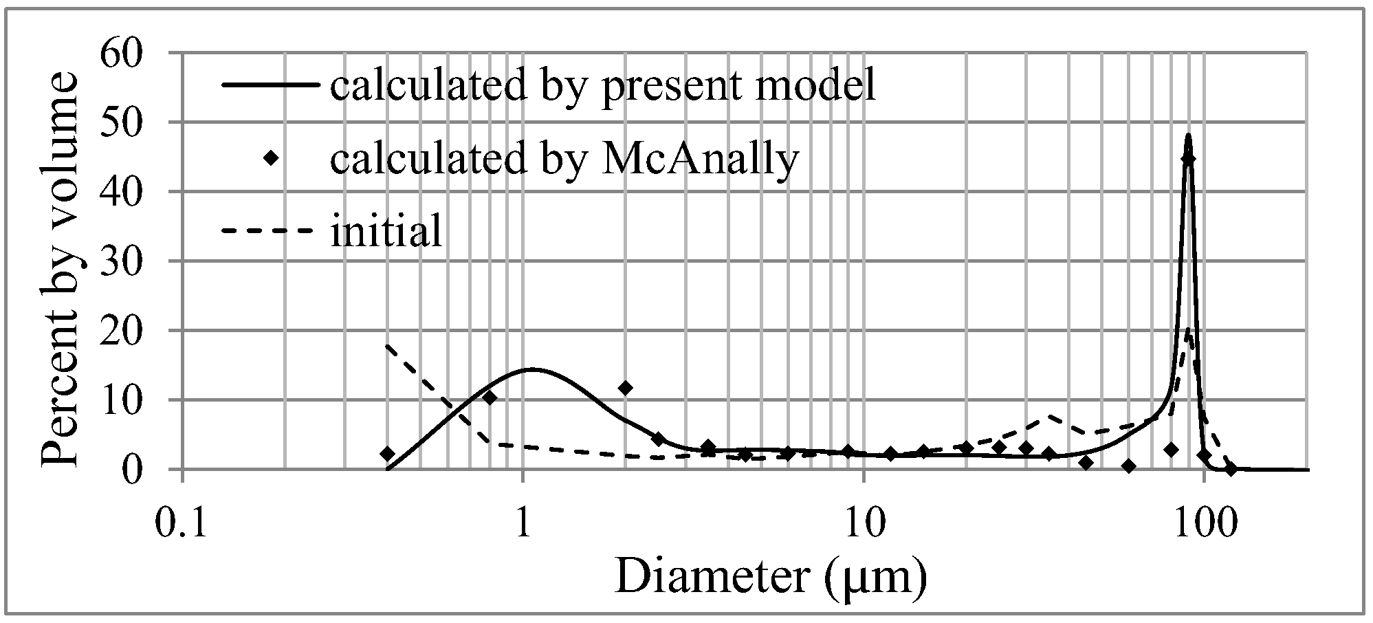
4.1. Aggradation Test of Non-Uniform Sediment

The capacity of the model to simulate non-uniform sediment deposition was validated by comparing the simulated results with experimental data obtained by McAnally [40].

The experimental flume used by McAnally was 100 m long and 0.23 m wide. The inflow condition was obtained by injecting fine sediment slurry into a steady flow. The water depth at the outlet of flume was maintained at 15.2 cm by a tailgate. A summary of sediment experimental conditions is given in

Table 1. Conditions for McAnally’s experiments and numerical simulation.

Experiment Number	Sediment	Inflow Concentration kg/m3	Flow Rate m3/s	Slurry Temperature deg C	Duration h	Manning’s Roughness Coefficient
W4	Kaolinite	10	0.0052	27	1.5	0.020
W5	Kaolinite	10	0.0070	27	1.0	0.021
W6	Kaolinite	10	0.0034	29	1.0	0.021
W9	Kaolinite	2	0.0034	27	1.25	0.022
W10	Kaolinite	5	0.0034	23	1.25	0.023
W11	Atchafalaya Bay Mud	10	0.0017	13	1.25	0.031

. Kaolinite was used in experiments W4 to W10, and Atchafalaya Bay mud was used in experiment W11. The grain size distributions of the kaolinite and Atchafalaya Bay mud are shown in Figure 1. Median diameters were approximately 1 μm for the kaolinite and 15 μm for the Atchafalaya Bay mud. The water used in the flume experiment had a pH of 7.8, 18.3 ppm of chloride, 13.1 ppm of sodium, and 1.9 ppm of calcium.

Figure 2 shows the sediment size distribution at the beginning of the experiment and the calculated sediment size distribution after 30 min, when a water–sediment parcel would have neared the end of the flume in experiment W11. The size distribution calculated by present model is similar to the results obtained by McAnally [40]; the distribution is bimodal, with the peak remaining at approximately 75 μm and the secondary peak moving toward larger sizes as ongoing aggregation of the smallest particles occurred.

Figure 3 shows McAnally observed and calculated depth-averaged sediment concentration profiles over the length of the flume, with laboratory observations depicted as solid points and calculated depth-mean profiles as lines. Figure 3 demonstrates that the computed sediment concentrations generally agree with the measured concentrations. These results indicate that the critical bed-shear stress for deposition used in this model, Formula (6), reasonably well represents the flocculation of fine particles.

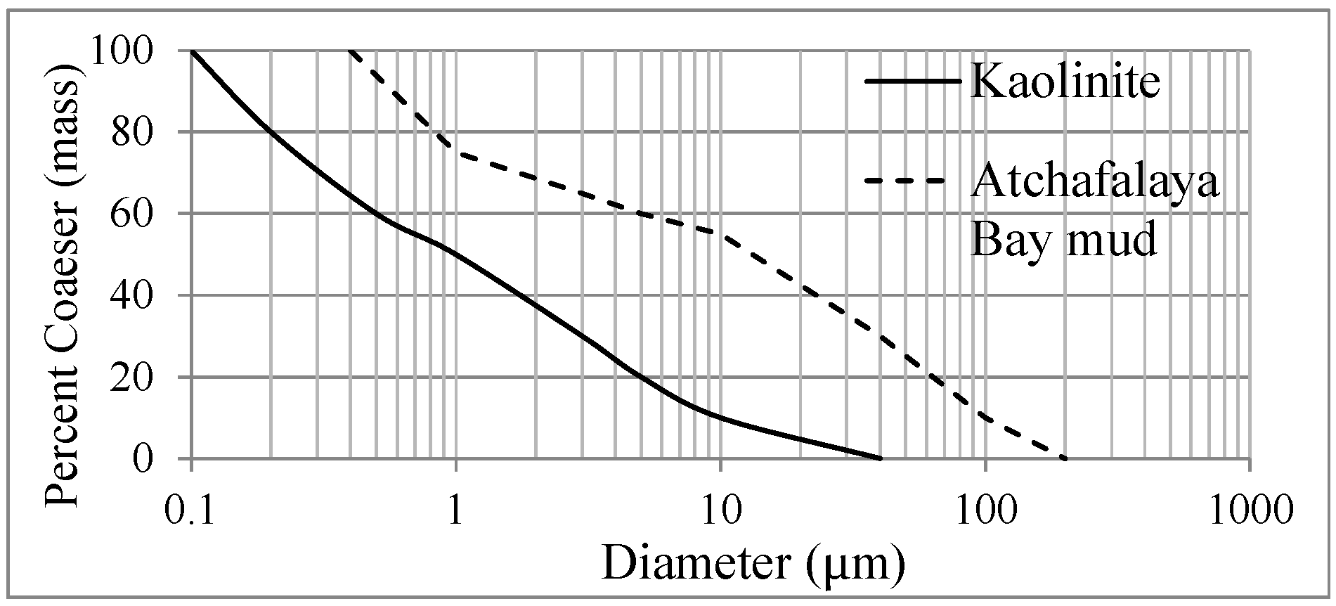
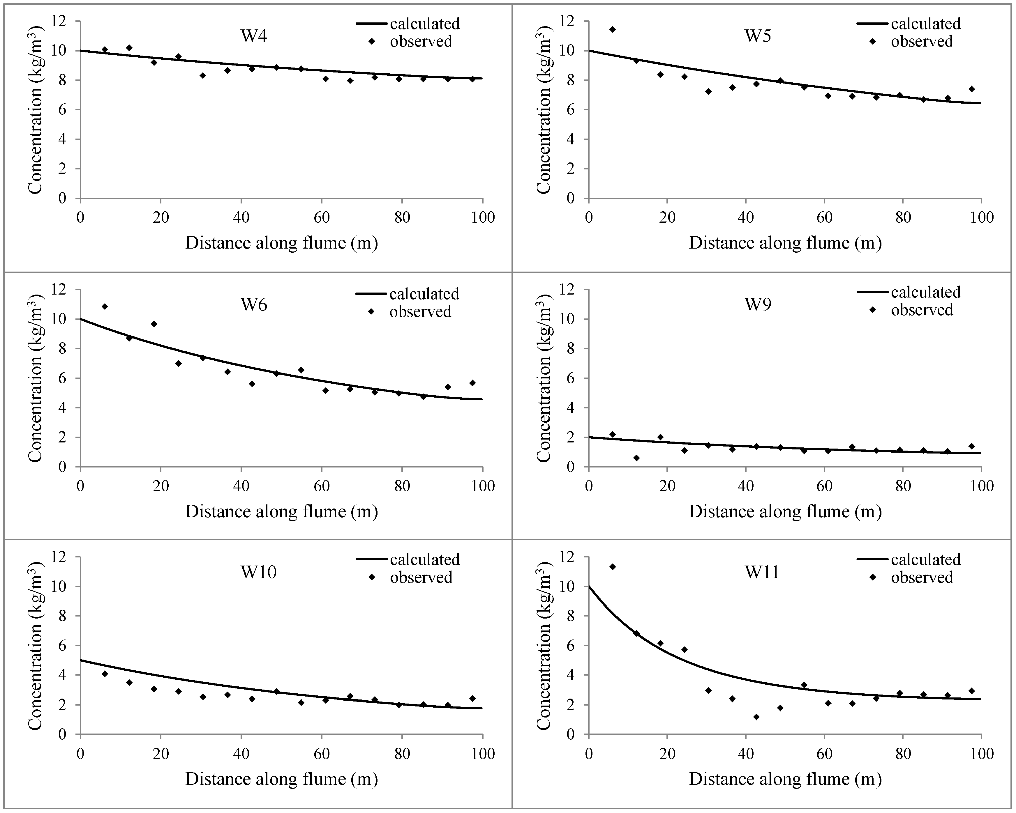
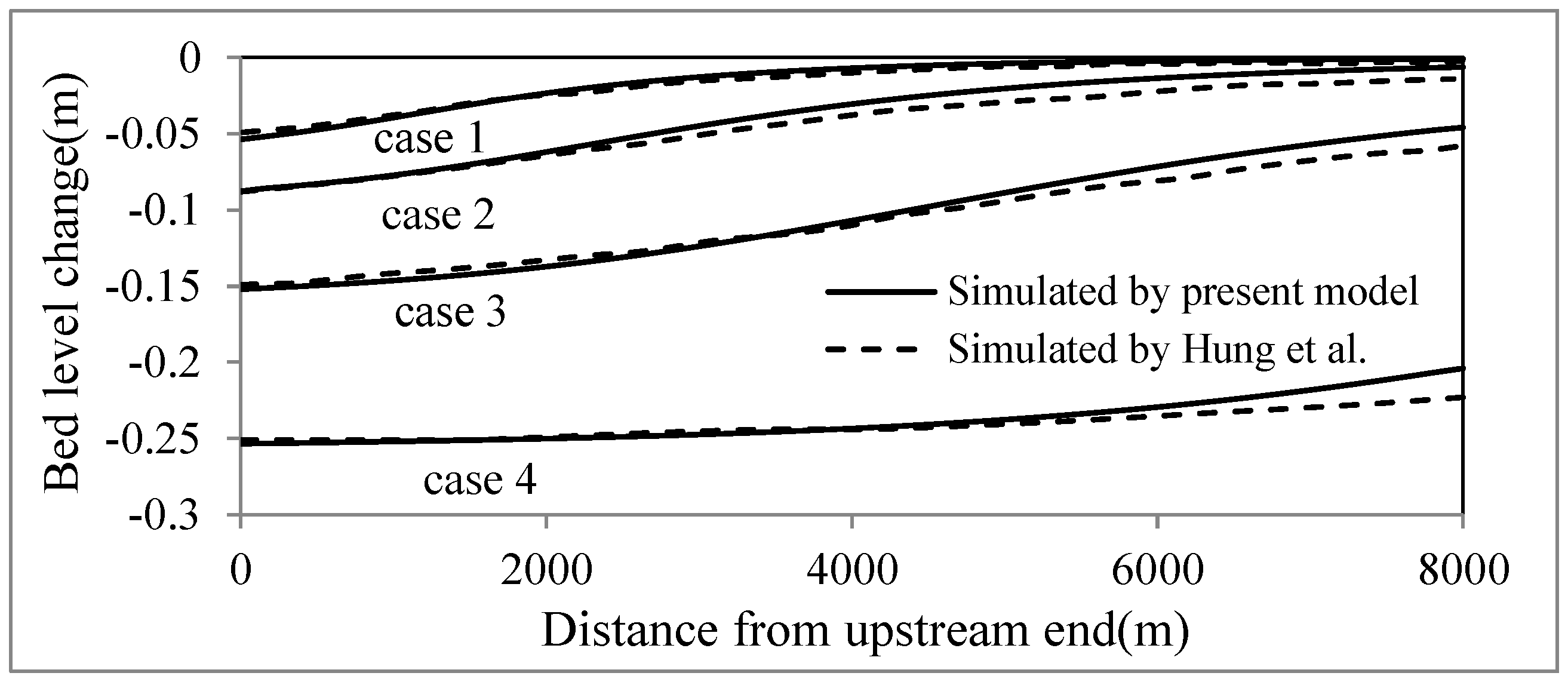
4.2. Erosion Test of Non-Uniform Sediment

Hung et al. [29] conducted an experiment for the erosion of cohesive non-uniform sediment. A straight rectangular channel was used with a length of 8000 m, a width of 100 m, a slope of 0.0005, and Manning’s roughness of 0.03. Three size classes of sediment were used in the study: 0.001 mm (clay, 33.33%), 0.01 mm (silt, 33.33%), and 0.05 mm (silt, 33.33%). The water surface elevation for the channel outlet was fixed at 4.5 m, and an initial sediment concentration of zero was used. The total simulation time was six days, and a grid of 81 × 11 cells was used in the simulation. The erosion experiment included four cases with a constant inflow sediment concentration of 2 kg/m³ and various inflow discharges Q (case1: Q = 100 m³/s; case2: Q = 200 m³/s; case3: Q = 400 m³/s; and case4: Q = 800 m³/s).

Figure 4 shows that the erosion depths simulated by the present model and Hung et al.’s are nearly equal near the channel inlet, but the absolute values from our model become smaller relative to Hung’s towards the outlet of the channel. A reasonable interpretation for this phenomenon is that the τek of our model is calculated using Formula (4) and considers the cohesive force in proportion to the water depth. In Hung’s model, a constant value was used for critical bed-shear stress for erosion along the channel. These results demonstrate that our model can simulate erosion of cohesive non-uniform sediment.

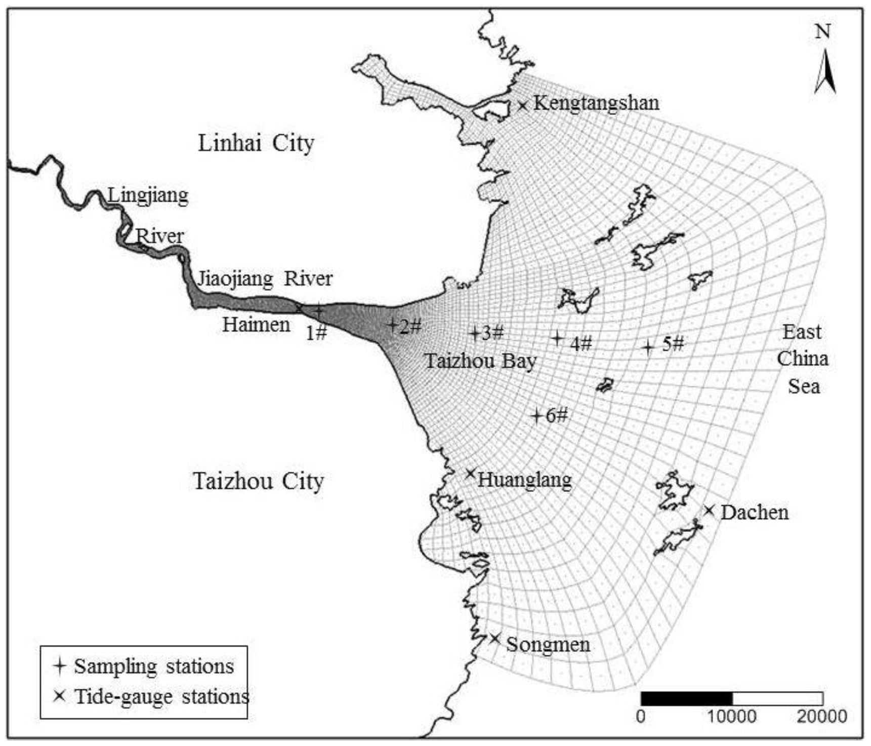
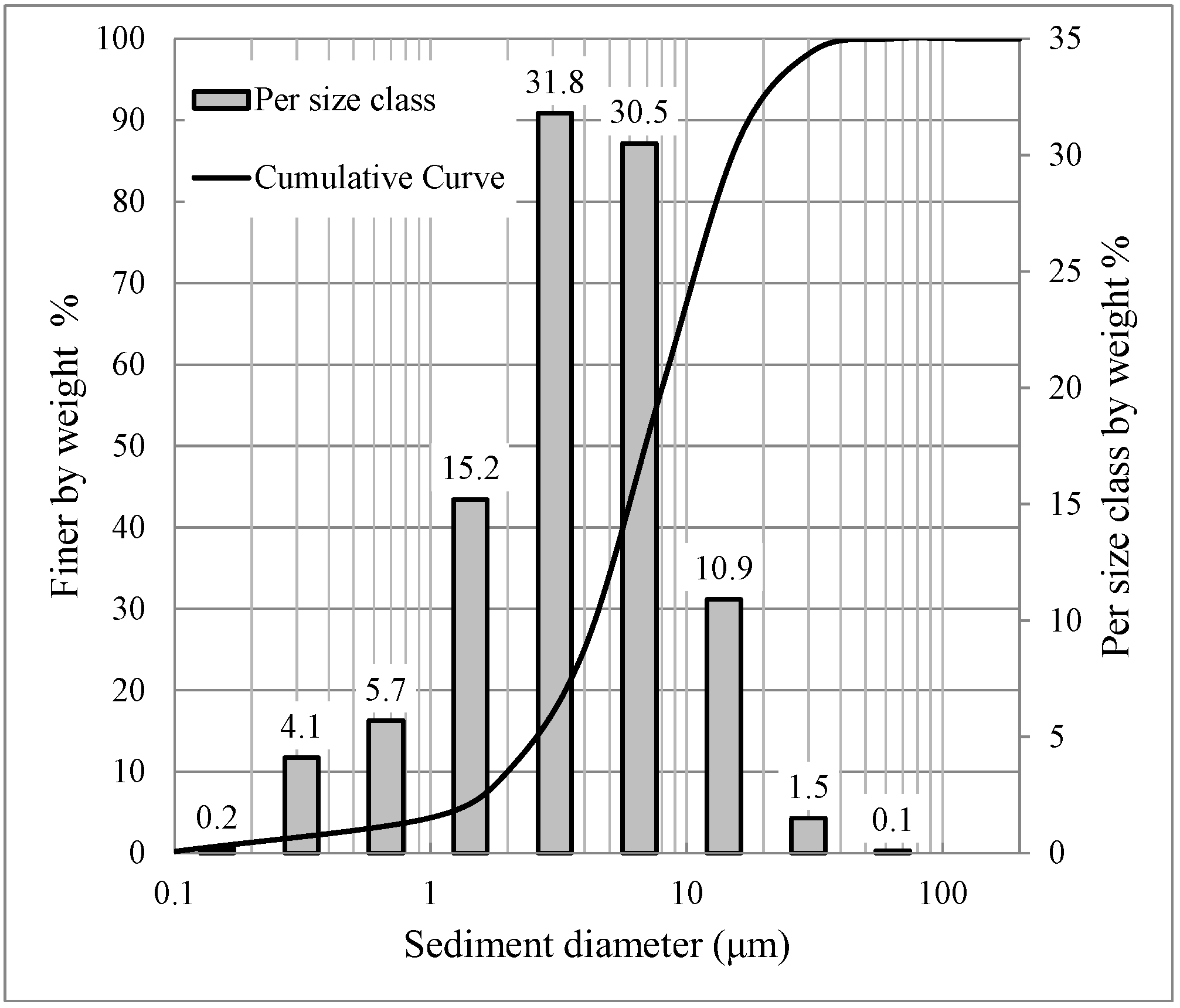
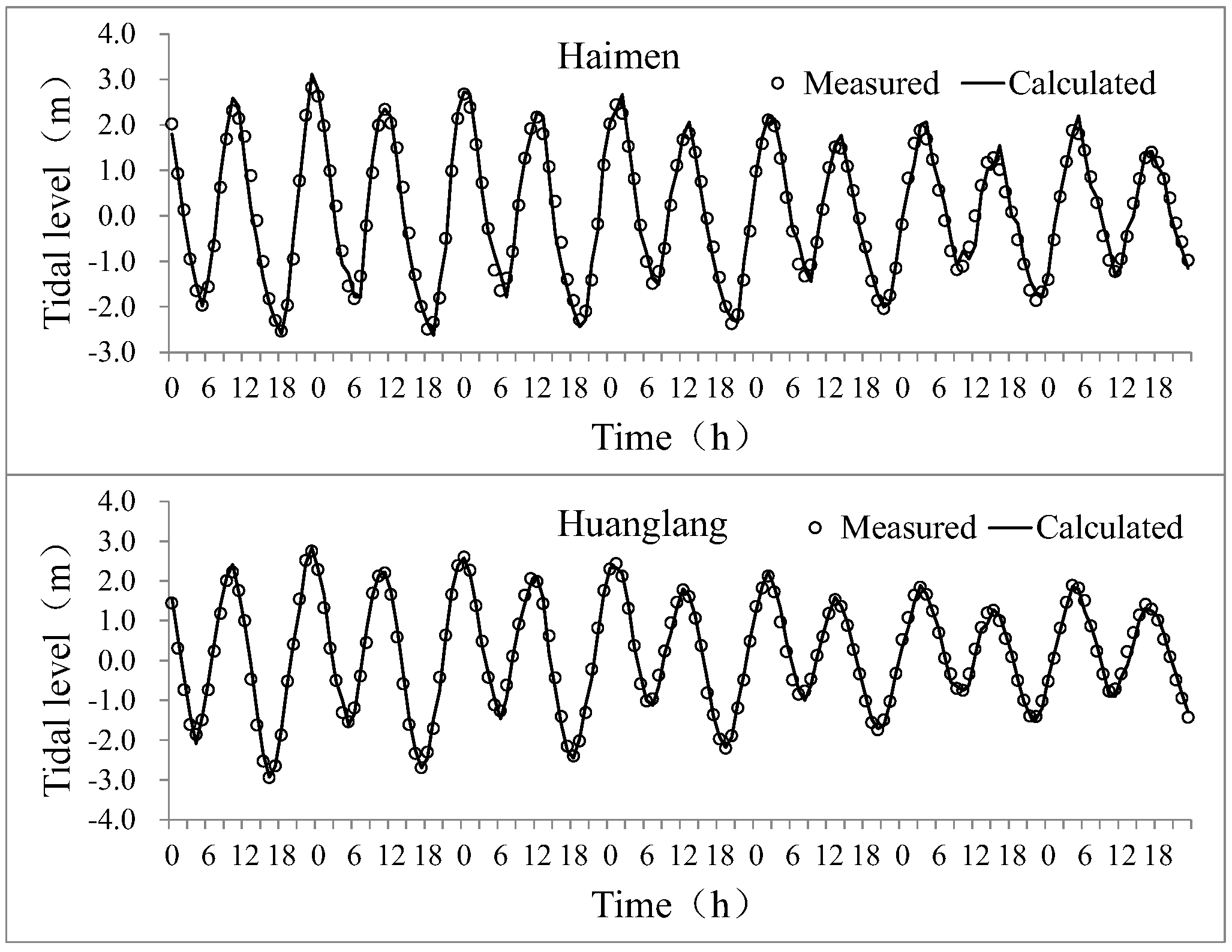
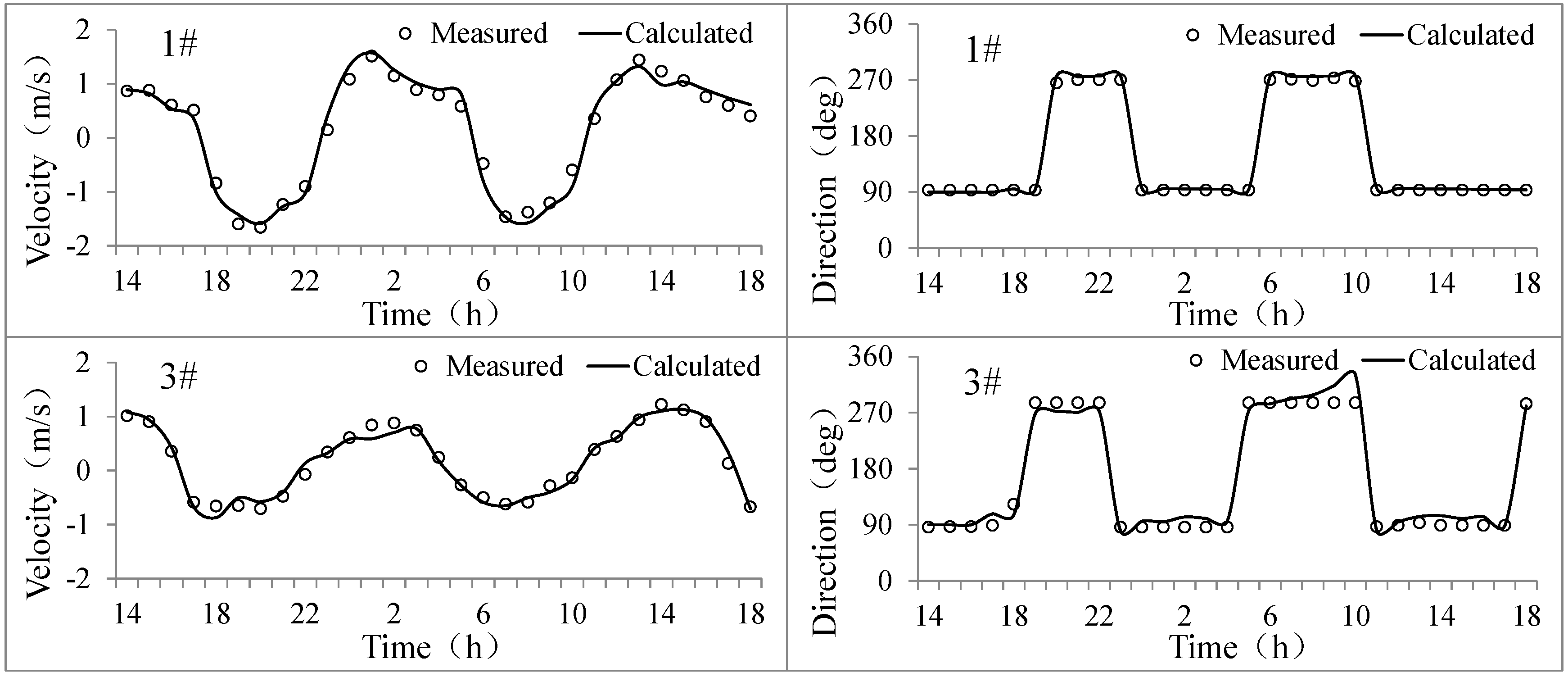
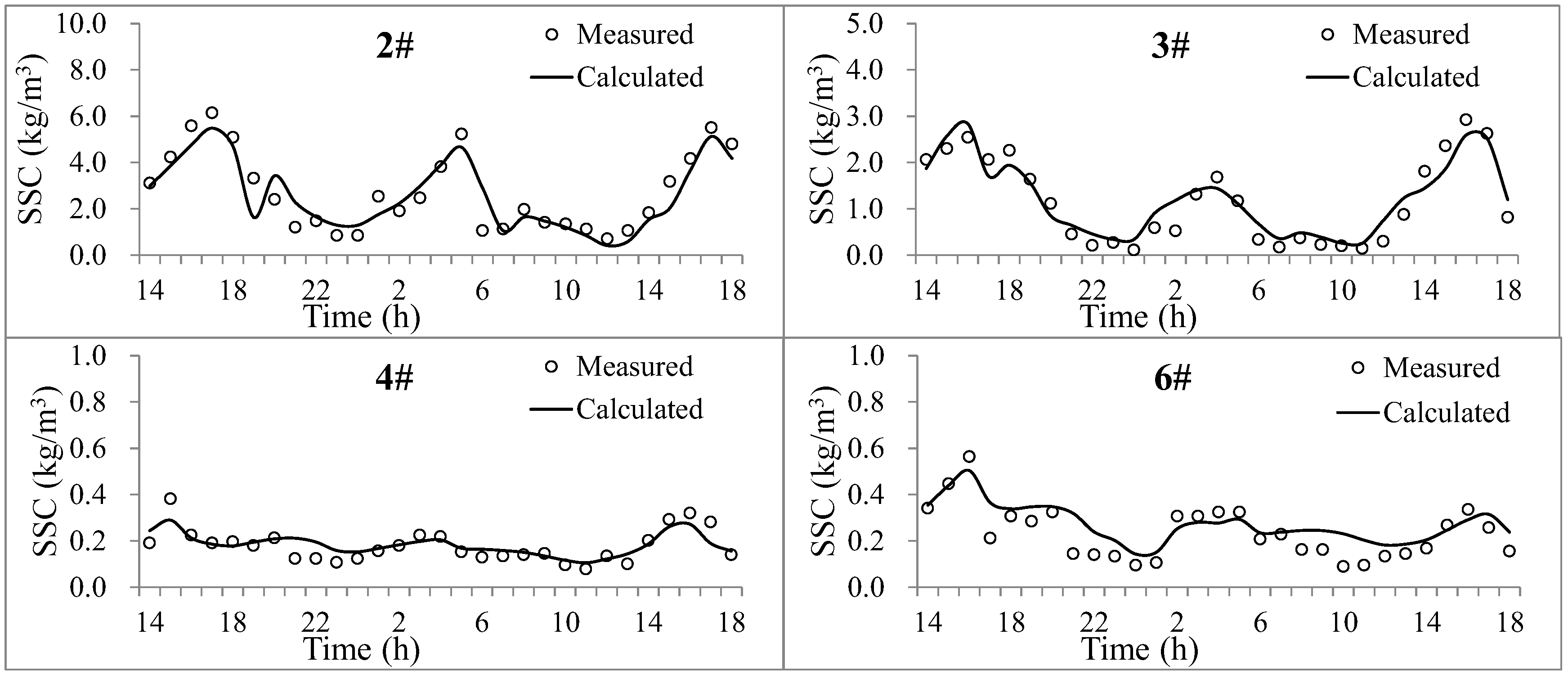
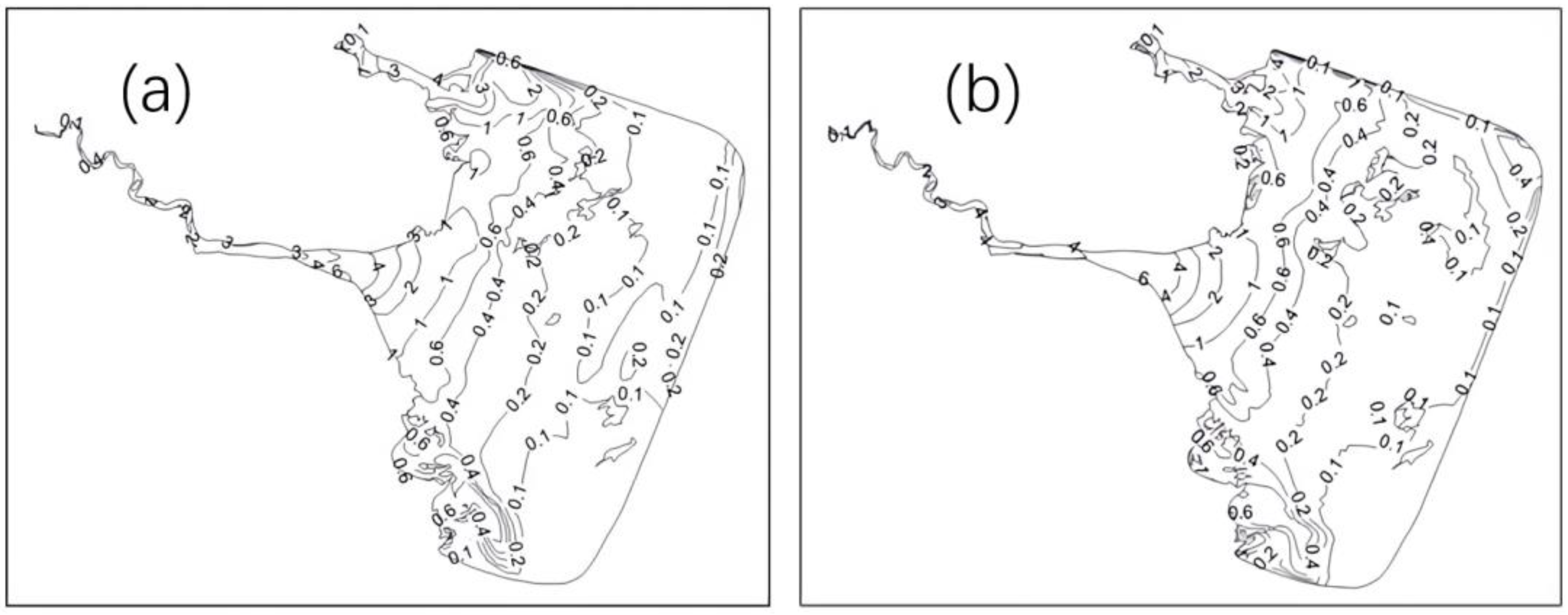
4.3. Simulation of Current and Sediment Transport in Jiaojiang Estuary

The Jiaojiang estuary, the third largest tidal estuary in Zhejiang Province, China, was chosen for model verification (Figure 5). It is a typical macro-tidal estuary with predominantly cohesive fine sediment. Samples from Jiaojiang estuary show that nearly 90% of the sediment is clay and fine silt with a diameter below 10 μm (Figure 6). More detailed information about Jiaojiang estuary is available from previous work [41,42]. The hydrology data from April to May 2009 were chosen for verification to match the topography data. The morphology data were obtained from measured data in 2009. A discharge per-cell boundary was applied at the upstream boundary, and a long-term tidal surface elevation signal was used downstream. Additionally, measured sediment concentration profile was applied at the upstream boundary, and downstream sediment flux was obtained from sediment sampling stations. Based on the grading curve shown in Figure 6, five different sediment classes were chosen as representative sediment classes of the non-uniform sediment: 0.0014 mm, 10%; 0.004 mm, 15.2%; 0.016 mm, 30.5%; 0.031 mm, 12.5%. The grid cell sizes in the computation are 20–200 m within the Jiaojiang estuary mouth and 200–3500 m in the outer sea (Figure 5). The total area of the computational domain is approximately 2500 km². The time step is 10 s. Based on the available observations, the open boundary upstream of Jiaojiang River is controlled by water discharge, and the outer sea boundaries are governed by tidal elevations in the hydrodynamic simulations. The average size distribution of sediment samples was set as the initial sediment gradation.

The model was validated by tidal levels from 27 April to 3 May 2009, as well as the current (speed and direction) and suspended sediment concentrations (SSC) during spring tide. Figure 7 compares the computed and observed tidal levels at several stations. The computed results are in good agreement with the measured values. Figure 8 compares calculated to measured flow velocities and directions, showing that both the magnitude and the direction of the computed velocity match the field data at each station. Thus, the present model is well suited to simulate tidal currents.

The time series of computed and measured SSC is shown in Figure 9. In general, simulated SSC is in agreement with measured SSC. Figure 10a,b indicate the simulated SSC distribution at the flood and ebb during spring tide, respectively. The turbidity maximum zone of Jiaojiang estuary is reasonably duplicated by the model, as shown in Figure 10a,b. These results demonstrate that the present model, which uses Sun’s theories for non-uniform sediment transport, has the capacity to simulate non-uniform sediment transport in estuaries.

5. Conclusions

In this paper, a depth-averaged two-dimensional model for the simulation of tidal current and non-uniform sediment transport in estuaries was developed based on a series of formulas proposed by Sun [1,2,3,4,5]. We firstly evaluate and discuss several key parameters for non-uniform sediment transport, including the critical bed-shear stress for erosion and deposition, erosion coefficients, and the settling velocity. The critical bed-shear stress for erosion and deposition deduced from the incipient probability of non-uniform sediment are able to describe both cohesive and noncohesive non-uniform sediment transport. Erosion coefficients are derived from experimental data on the scour of drilling samples from the Qiantang River estuary. The settling velocity formula is adequate for particles of any size and various passing flow states.

Results from this model are compared with several datasets, including both an aggradation and an erosion experiment. Good performance in the tests indicates that the model can simulate the aggradation and erosion processes of non-uniform sediment. The model is also verified using measured data from Jiaojiang estuary, and the computed results agree well with the measured values. The model can reasonably replicate the turbidity maximum zone of Jiaojiang estuary. The proposed model is able to simulate the flow and non-uniform sediment transport in tidal estuaries.

References

1. Cao, Z.; Carling, P.A. Mathematical modelling of alluvial rivers: Reality and myth. Part 1: General review. In Proceedings of the Institution of Civil Engineers-Water and Maritime Engineering; Thomas Telford Ltd.: London, UK, 2002; Volume 154, pp. 207–219. [Google Scholar]
2. Papanicolaou, A.N.; Elhakeem, M.; Krallis, G.; Prakash, S.; Edinger, J. Sediment transport modeling review—Current and future developments. J. Hydraul. Eng.-ASCE. 2008, 134, 1–14. [Google Scholar] [CrossRef]
3. Juez, C.; Ferrer-Boix, C.; Murillo, J.; Hassan, M.A.; García-Navarro, P. A model based on Hirano-Exner equations for two-dimensional transient flows over heterogeneous erodible beds. Adv. Water Resour. 2016, 87, 1–18. [Google Scholar] [CrossRef] [Green Version]
4. Cao, Z.; Hu, P.; Pender, G.; Liu, H.H. Non-capacity transport of non-uniform bed load sediment in alluvial rivers. J. Mt. Sci. 2016, 13, 377–396. [Google Scholar] [CrossRef]
5. Navas-Montilla, A.; Juez, C.; Franca, M.J.; Murillo, J. Depth-averaged unsteady RANS simulation of resonant shallow flows in lateral cavities using augmented WENO-ADER schemes. J. Comput. Phys. 2019, 395, 511–536. [Google Scholar] [CrossRef]
6. Portela, L.I. Non-uniform modelling of suspended sediment transport in the Tagus estuary. WIT Trans. Ecol. Environ. 2000, 40, 1–8. [Google Scholar]
7. Fischer-Antze, T.; Rüther, N.; Olsen, N.R.B.; Gutknecht, D. Three-dimensional (3D) modeling of non-uniform sediment transport in a channel bend with unsteady flow. J. Hydraul. Res. 2009, 47, 670–675. [Google Scholar] [CrossRef]
8. Tritthart, M.; Schober, B.; Liedermann, M.; Habersack, H. Numerical modeling of sediment transport in the Danube River: Uniform vs. non-uniform formulation. River Flow 2010, 2010, 977–984. [Google Scholar]
9. Tritthart, M.; Liedermann, M.; Schober, B.; Habersack, H. Non-uniformity and layering in sediment transport modelling 2: River application. J. Hydraul. Res. 2011, 49, 335–344. [Google Scholar] [CrossRef]
10. Jha, S.K.; Bombardelli, F.A. Theoretical/numerical model for the transport of non-uniform suspended sediment in open channels. Adv. Water Resour. 2011, 34, 577–591. [Google Scholar] [CrossRef]
11. Novák, P.; Čabelka, J. Models in Hydraulic Engineering: Physical Principles and Design Applications; Pitman Publishing: London, UK, 1981. [Google Scholar]
12. Davinroy, R.D. Physical Sediment Modeling of the Mississippi River on a Micro Scale. Master’s Thesis, University of Missouri, Rolla, MO, USA, 1994. [Google Scholar]
13. Maynord, S.T. Evaluation of the micromodel: An extremely small-scale movable bed model. J. Hydraul. Eng. 2006, 132, 343–353. [Google Scholar] [CrossRef]
14. Afzal, M.S.; Holmedal, L.E.; Myrhaug, D. Sediment transport in combined wave–current seabed boundary layers due to streaming. J. Hydraul. Eng. 2021, 147, 04021007. [Google Scholar] [CrossRef]
15. Afzal, M.S. 3D Numerical Modelling of Sediment Transport under Current and Waves. Master’s Thesis, Institutt for Bygg, Anlegg og Transport, Trondheim, Norway, 2013. [Google Scholar]
16. Pourshahbaz, H.; Abbasi, S.; Pandey, M.; Pu, J.H.; Taghvaei, P.; Tofangdar, N. Morphology and hydrodynamics numerical simulation around groynes. ISH J. Hydraul. Eng. 2022, 28, 53–61. [Google Scholar] [CrossRef]
17. Lu, Y.J.; Li, H.L.; Dong, Z.; Lu, J.Y.; Hao, J.L. Two-Dimensional Mathematical Model of Tidal Current and Sediment for Oujiang Estuary and Wenzhou Bay. China Ocean. Eng. 2002, 16, 107–122. [Google Scholar]
18. Wu, W. Depth-averaged two-dimensional numerical modeling of unsteady flow and nonuniform sediment transport in open channels. J. Hydraul. Eng. 2004, 130, 1013–1024. [Google Scholar] [CrossRef]
19. Wang, S.Y. Depth-averaged 2-D calculation of tidal flow, salinity and cohesive sediment transport in estuaries. Int. J. Sediment Res. 2004, 19, 172–190. [Google Scholar]
20. Fang, H.W.; Wang, G.Q. Three-dimensional mathematical model of suspended-sediment transport. J. Hydraul. Eng. 2000, 126, 578–592. [Google Scholar] [CrossRef] [Green Version]
21. Hongwei, F.; Minghong, C.; Qianhai, C. One-dimensional numerical simulation of non-uniform sediment transport under unsteady flows. Int. J. Sediment Res. 2008, 23, 316–328. [Google Scholar]
22. Hung, M.C.; Hsieh, T.Y.; Wu, C.H.; Yang, J.C. Two-dimensional nonequilibrium noncohesive and cohesive sediment transport model. J. Hydraul. Eng. 2009, 135, 369–382. [Google Scholar] [CrossRef] [Green Version]
23. Xiao, Y.; Wang, H.; Shao, X. 2D numerical modeling of grain-sorting processes and grain size distributions. J. Hydro-Environ. Res. 2014, 8, 452–458. [Google Scholar] [CrossRef]
24. Peng, H.; Cao, Z.; Pender, G.; Liu, H. Numerical modelling of riverbed grain size stratigraphic evolution. Int. J. Sediment Res. 2014, 29, 329–343. [Google Scholar]
25. Qian, H.; Cao, Z.; Pender, G.; Liu, H.; Hu, P. Well-balanced numerical modelling of non-uniform sediment transport in alluvial rivers. Int. J. Sediment Res. 2015, 30, 117–130. [Google Scholar] [CrossRef]
26. Sun, Z.L. The General Law for the Fall Velocity of Particle in Quiescent Water. J. Hangzhou Univ. 1990, 17, 246–255. (In Chinese) [Google Scholar]
27. Sun, Z.L.; Xie, J.H.; Duan, W.Z.; Xie, B.L. Incipient motion of any fraction of non-uniform sediment. J. Hydraul. Eng.-Beijing. 1997, 10, 25–32. (In Chinese) [Google Scholar]
28. Sun, Z.; Donahue, J. Statistically derived bedload formula for any fraction of nonuniform sediment. J. Hydraul. Eng. 2000, 126, 105–111. [Google Scholar] [CrossRef]
29. Sun, Z.; Sun, Z.; Donahue, J. Equilibrium bed-concentration of nonuniform sediment. J. Zhejiang Univ.-SCIENCE A. 2003, 4, 186–194. [Google Scholar] [CrossRef]
30. Sun, Z.L.; Huang, S.H.; Zhu, L.L. Incipient probability of cohesive non-uniform sediment. J. Zhejiang Univ. Eng. Sci. 2007, 41, 18–22. (In Chinese) [Google Scholar]
31. Sun, Z.L.; Zhang, C.C.; Huang, S.H.; Liang, X. Scour of cohesive non-uniform sediment. J. Sediment Res. 2011, 44–48. (In Chinese) [Google Scholar]
32. Sun, Z.L.; Ni, X.J.; Xu, D.; Nie, H. Some problems on mathematical model of sediment transport in estuary. J. Zhejiang Univ. Eng. Sci. 2015, 49, 231–236. (In Chinese) [Google Scholar]
33. Tayfur, G. Empirical, numerical, and soft modelling approaches for non-cohesive sediment transport. Environ. Process. 2021, 8, 37–58. [Google Scholar] [CrossRef]
34. Krone, R.B. Flume Studies of the Transport of Sediment in Estuarial Shoaling Processes; Hydraulic and Sanitary Engineering Laboratory, University of California: Berkeley, CA, USA, 1962. [Google Scholar]
35. Zhang, R.J.; Xie, J.H. River Sediment Transport; China Water and Power Press: Beijing, China, 1997. (In Chinese) [Google Scholar]
36. van Maren, D.S.; Winterwerp, J.C.; Wu, B.S.; Zhou, J.J. Modeling hyperconcentrated flow in the Yellow River. Earth Surf. Process. Landf. 2009, 34, 596–612. [Google Scholar] [CrossRef]
37. Wu, W.M.; Vieira Dalmo, A.; Wang, S.S.Y. One-dimensional numerical model for non-uniform sediment transport under unsteady flows in channel networks. J. Hydraul. Eng.-ASCE 2004, 130, 914–923. [Google Scholar]
38. Wu, W.M.; Wang Sam, S.Y. Formulas for Sediment Porosity and Settling Velocity. J. Hydraul. Eng.-ASCE 2006, 132, 858–862. [Google Scholar] [CrossRef]
39. Lu, Q.M. Three-Dimensional Modeling of Hydrodynamics and Sediment Transport with Parallel Algorithm. Ph.D. Thesis, The Hong Kong Polytechnic University, Hong Kong, China, 1998. [Google Scholar]
40. McAnally, W.H. Aggregation and Deposition of Estuarial Fine Sediment; Army Engineer Research and Development Center: Vicksburg, MS, USA, 2000. [Google Scholar]
41. Guan, W.B.; Wolanski, E.; Dong, L.X. Cohesive Sediment Transport in the Jiaojiang River Estuary, China. Estuar. Coast. Shelf Sci. 1998, 46, 861–871. [Google Scholar] [CrossRef]
42. Li, B.G.; Eisma, D.; Xie, Q.C.; Kalf, J.; Li, Y.; Xia, X. Concentration, clay mineral composition and Coulter counter size distribution of suspended sediment in the turbidity maximum of the Jiaojiang river estuary, Zhejiang, China. J. Sea Res. 1999, 42, 105–116. [Google Scholar] [CrossRef]
Figure 1. Grain size distribution of sediment used in numerical simulation.
Applsci 13 04286 g001
Figure 2. Calculated size distribution of W11 at t = 30 min [40].
Applsci 13 04286 g002
Figure 3. Observed and calculated longitudinal depth-mean concentration profiles.
Applsci 13 04286 g003
Figure 4. Bed level change caused by different inflow discharges during the erosion test [29].
Applsci 13 04286 g004
Figure 5. Simulation domain and grids.
Applsci 13 04286 g005
Figure 6. Average size distribution of the sediment samples from the Jiaojiang estuary.
Applsci 13 04286 g006
Figure 7. Comparison of the computed and observed tidal levels.
Applsci 13 04286 g007
Figure 8. Comparison of the computed and observed tidal flow velocities.
Applsci 13 04286 g008
Figure 9. Comparison of the computed and observed SSC.
Applsci 13 04286 g009
Figure 10. (a) SSC distribution at the flood tide; (b) SSC distribution at the ebb tide.
Applsci 13 04286 g010