1. Introduction
NASA proposed the Integrated Vehicle Health Management Technology (IVHM) in 1992 to enhance spacecraft systems’ operation, maintenance, and decision-making activities. With the passage of time, this concept underwent numerous iterations, and in 2020, it evolved into Intelligent Health and Task Management (IHMM), which is the latest technology available today [
1]. According to the International Aviation Association (IATA) 2018 report, the aerospace industry invested a whopping
$76 billion in vehicle overhauls in 2017 [
2]. This highlights the growing significance of fault prognosis and health management technology, which has become a crucial aspect of several industrial sectors, including aerospace. As modern industries continue to evolve and develop, comprehensive health management and diagnosis have become integral to maintaining the system’s operational life cycle. The field of prognostic health management is increasingly turning towards deep learning, which is gaining more attention due to its remarkable classification and feature extraction capabilities [
3].
The control Moment Gyroscope (CMG) is a vital component of large-scale and long-life spacecraft attitude adjustment systems. It comprises a high-speed rotor system and a servo frame system, which use angular momentum exchange with the spacecraft to execute attitude adjustments. To ensure the smooth operation of CMG, several key operating data, such as rotor motor current, rotor speed, frame servo motor current, frame angle, frame command, and shaft temperature, must be meticulously monitored and controlled. Additionally, the spacecraft attitude and motion data can be used as a reference to assist in determining whether the system is functioning normally. The stable and consistent operation of CMG is critical to the successful completion of the spacecraft’s mission. Early troubleshooting is essential, and anomaly detection plays a crucial role in identifying and resolving potential issues in a timely and efficient manner [
3,
4,
5].
Health management refers to diagnosing and preventing system failure while predicting the reliability and remaining useful life of its components. In the past few decades, systematic health management research has been a popular direction. Much of the initial research focused on addressing the different failures that occur at the component level and at the system level. The attention of researchers since then has focused on the integration of anomaly, diagnostics, and prediction techniques across systems and related platforms. Fault diagnosis and health management technology has been developed in three directions over the years, namely model-based [
6], knowledge [
7], and data-driven methods [
8,
9,
10,
11]. Compared with methods such as model-based methods or knowledge-based expert systems, data-driven methods do not require the establishment of accurate models, and there is no bottleneck in knowledge acquisition. A data-driven approach is a new paradigm of bottom-up solutions [
3]. It can save a lot of manpower and material resources related to knowledge acquisition or accurate model establishment.
Therefore, fault prognosis and health management based on deep learning have entered people’s field of vision. Deep learning is a field in machine learning, which uses deep artificial neural networks to learn the inherent laws and representation levels of data, and build models for feature extraction and task execution. Anomaly detection based on deep learning can more efficiently and accurately extract anomaly information and prevent early failures from the current large-scale spacecraft telemetry data [
12]. The deep learning methods suitable for spacecraft telemetry time series data mainly include Recurrent Neural Network (RNN), Long Short-Term Memory (LSTM), Gated Recurrent Unit (GRU), and so on [
13]. Among them, LSTM has the ability to maintain long-term information memory, which has huge advantages in the fields of Natural Language Processing (NLP), speech recognition, and time series prediction [
14]. In addition, in the work of speech recognition, SincNet has also achieved great success due to its special filter structure and interpretability. This is a great inspiration for working with time series data [
15].
Since the working states of various systems and machines are stable most of the time, the scarcity of labeled data has become one of the data problems in the field of fault detection and anomaly detection. The absence of large labeled datasets has led researchers to turn their attention to Transfer Learning (TL) [
16,
17]. Transfer learning transfers knowledge in related but different domains to improve the learning machine’s ability to complete related tasks in the target domain [
18]. According to the feature space and label space of the target and source domains in transfer learning, transfer learning can be divided into homogeneous transfer learning and heterogeneous transfer learning. If the feature space of the target and source domains is
and the label space
; this situation is called isomorphic transfer learning. If
or
, then this situation is called heterogeneous transfer learning. According to the knowledge transfer strategy, transfer learning can also be divided into four transfer methods: instance-based, feature-based, parameter-based, and model-based [
19].
Transfer learning not only solves the problem of less labeled data in the field of fault and anomaly detection but also can greatly shorten the model convergence time through pre-training and other means. One of the main characteristics of fault diagnosis tasks is the imbalance of fault data. Models trained on smaller datasets generally generalize poorly and are prone to overfitting, so pre-training on larger datasets is needed for knowledge transfer. Whether in the military field or in the civilian field, it is of great significance to quickly adapt to new problems that arise.
Operating a spacecraft is a complex, multi-stage process that spans a long cycle. It involves ground launch, acceleration and escape, deceleration and berthing into orbit, attitude adjustment, and more. Despite the lack of an atmospheric environment, space poses extreme temperatures and exposure to cosmic rays, both of which can impact the spacecraft’s components and performance over time. To ensure the spacecraft’s reliable operation, it is crucial to study the conditions that lead to anomalies. These conditions include the spacecraft’s environmental state (e.g., temperature, radiation) and mission state (e.g., acceleration, deceleration, attitude adjustment). By classifying and studying different working conditions, we can more precisely monitor the spacecraft’s health status and prevent or eliminate faults. Furthermore, by modeling the spacecraft’s operation data under different working conditions, we can improve the accuracy and recall rate of anomaly detection while minimizing false positives and missed detections.
Based on the reference of the above fields for spacecraft anomaly detection methods, this paper proposes a Sinc-LSTM neural network for spacecraft actuator anomaly detection based on transfer learning and working condition classification. We selected the important inertial actuator CMG of the spacecraft as the research object. In the field of spacecraft anomaly detection, labeled data is generally insufficient to support model establishment, so a transfer learning method is introduced to introduce anomaly knowledge of different spacecraft into model tasks. The main contributions of this paper are as follows:
- (1)
The anomaly detection of CMG data is carried out using the transfer learning method, and a two-stage pre-training is designed. The features of general time series data and the features of the same type of spacecraft are extracted respectively to solve the problems of less CMG public data, difficult modeling, and less labeled data.
- (2)
A Sinc-LSTM network is designed for fitting and reconstructing time series data in anomaly detection. Since filters can add interpretability to neural networks and improve their ability to fit time series data. LSTM, which can retain long-term information, is crucial for accurately fitting and reconstructing long-period data. The proposed network aims to achieve better performance in time series data fitting and reconstruction for anomaly detection.
- (3)
The data classification is completed with automatic clustering, and a dynamic threshold judgment mechanism is set up, which adds environmental awareness to the anomaly detection model, which can improve the accuracy of network detection and reduce misjudgments.
2. Background and Related Works
The stability of spacecraft in orbit is an important guarantee for the completion of space missions. In order to avoid the extreme impact and huge cost after failure, the technology of Prognostics and Health Management (PHM) of spacecraft has been proposed to deal with it. PHM predicts the future product reliability by evaluating the deviation or degradation degree of the product from the expected normal operating state, and measures, records, and monitors the deviation and degradation degree of the normal operating state in real time [
20]. CMG is an inertial actuator to help spacecraft complete attitude adjustment, and is the “fulcrum” generated by a spacecraft in the weightless environment in space [
21]. Anomaly detection of CMG is a key part of the health management of the whole spacecraft system.
The performance of spacecraft anomaly detection is often affected by working conditions, and the setting of anomaly detection model parameters will be quite different under different working conditions. In addition, for data-driven anomaly detection methods, the detection model learned under one working condition usually cannot be well generalized to another [
22]. Therefore, it is very necessary to propose targeted anomaly detection strategies for spacecraft under different working conditions. In addition, due to the special nature of spacecraft data, very little data is available on CMG. The particularity of anomaly detection data also determines that it is difficult to obtain the annotated data. Therefore, it is better to obtain partial prior knowledge using transfer learning.
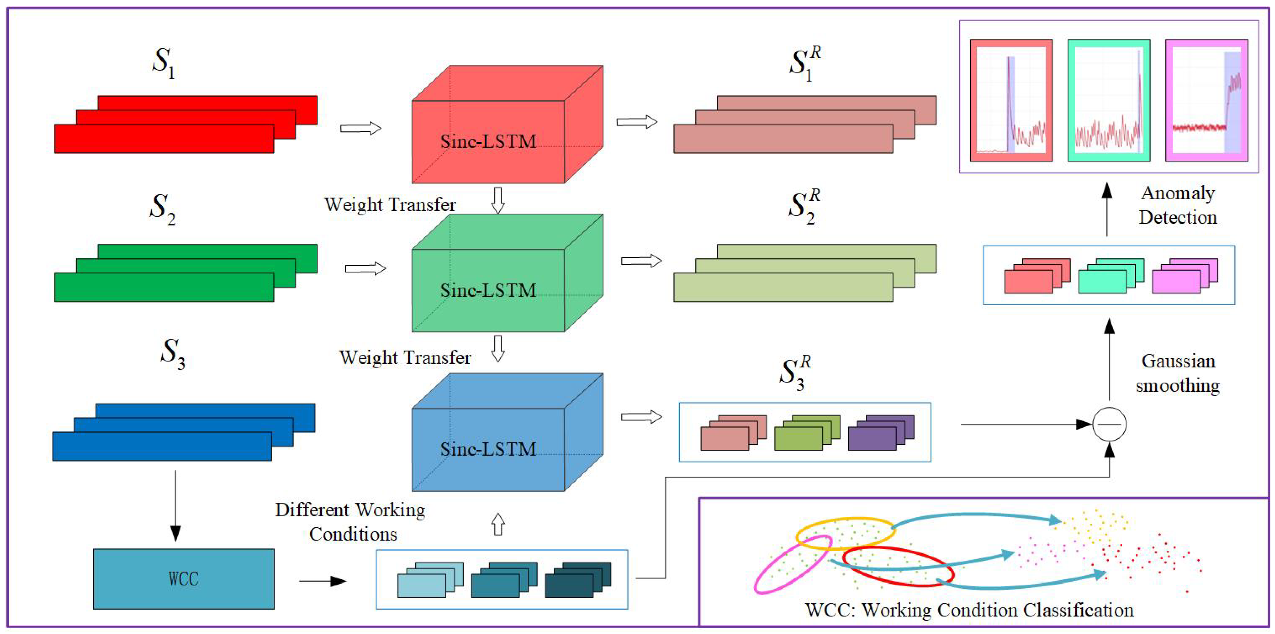
Based on the above analysis, we designed the anomaly detection process shown in
Figure 1. The Sinc-LSTM time series reconstruction network is designed by combining SincNet with LSTM. Before Sinc-LSTM is trained by CMG data, it is pre-trained in two stages by two open access datasets (
and
, which will be introduced in the
Section 3). Before CMG data (
) is input into the network, the peak density clustering method is used to segment the working conditions. The reconstructed time series data (
) is obtained after the network is trained by CMG data from each working condition. Subtracting
from the original data yields a sequence of differences. The result of anomaly detection can be obtained by threshold judgment on the difference sequence after Gaussian smoothing. In this section, the related work is briefly introduced to analyze the advantages of the proposed method.
2.1. Working Conditions Classification
In the mission cycle of a spacecraft, there are many different working stages. In space, different environments can also cause different disturbances to a spacecraft. The influence of the space environment mainly comes from the electromagnetic environment, atmospheric environment, space debris, and the influence of the position of other celestial bodies [
23].
The electromagnetic environment of space will interfere with the electromagnetic system of a spacecraft. After the interaction between plasma and surface materials, the spacecraft will be charged, and the accumulated strong electric field will break down the electronic components inside the spacecraft. The solar radiation pressure will generate mechanical forces, which will seriously affect the attitude stability of the spacecraft [
24]. Space atmosphere has different effects on a spacecraft in different layers. The drag force of the upper atmosphere is the main orbital perturbation force of a low orbit spacecraft [
25]. When the shape of the spacecraft is asymmetric in the relative direction of motion, the drag force of the upper atmosphere will generate torque and affect the attitude control of the spacecraft. The atomic oxygen produced by the interaction between solar ultraviolet and oxygen molecules also has a serious denudation and aging effect on the structure of low-orbit spacecraft. Space debris of different scales and velocities can cause erosion or structural damage to a spacecraft. The position of the relative celestial body mainly affects the celestial body sensor used for attitude determination on the spacecraft.
The operation of a spacecraft is a long cycle process, divided into different stages, and will face a different mission environment and mission intensity. The working condition of the spacecraft is defined as the set of the environment state (temperature, electromagnetic radiation intensity), mission state (acceleration, deceleration, attitude adjustment), and life cycle (service time) of the spacecraft, covering all the factors that may affect the threshold of spacecraft anomaly detection. The performance of spacecraft anomaly detection can be improved by classifying the working conditions of the spacecraft. Targeted fault detection under different working conditions has shown advantages in multiple tasks [
22,
26,
27,
28]. Reference work [
22] points out that the residual life estimation model of bearings trained under a single working condition cannot be well generalized to bearings under other working conditions. Therefore, a transfer learning method based on a multi-layer perceptron is proposed, which can adaptively complete the detection of bearing fault occurrence time under different working conditions.
2.2. PHM of CMG
As mentioned in the first part, CMG is the inertial actuator of the spacecraft, and the spacecraft performs attitude adjustment based on CMG through angular momentum transfer. The fault prediction and health management technology of CMG is the key to the stable operation of spacecraft in orbit. Two of the four CMGs used by the International Space Station failed unexpectedly after 1.3 and six years of service, respectively, and both crews had to return to Earth for investigation [
29]. The PHM problem of CMG mainly focuses on anomaly detection and fault isolation. Data to watch include speed, shaft temperature, current, frame angle, and commands.
The anomaly detection methods of CMG have evolved from the early expert manual-based methods to data-driven based methods. Reference work [
30] proposed an adaptive threshold fault detection, identification, and isolation algorithm, which combined lossless Kalman filter with residual and innovation sequence, and used binary grid search method to detect the fault and then adapted to jointly estimate the covariance matrix of a Kalman filter. In reference work [
5], a chaotic integration method of an online cyclic extreme learning machine is proposed to predict and reconstruct the temperature signal of a controlling torque gyroscope. The model can predict temperature dynamically and overcome the nonlinear and chaotic characteristics of the CMG temperature signal. Reference work [
4,
31] proposes a data-driven method that integrates the symmetry and orientation attributes of satellite attitude rate data into the neural network model, greatly reducing the need for historical data. In reference work [
32], physical information is integrated into neural networks, and a neural network inspired by the physical mechanism of CMG is designed, which integrates various types of data to detect anomalies in CMG, and fine-adjusts by adopting transfer learning. This method integrates prior knowledge into neural networks and explores the fusion of data-driven and physical model methods for anomaly detection.
In reference work [
9], the wavelet denoising method and Short-Time Fourier Transform (STFT) are utilized to preprocess the signal of CMG to obtain the frequency spectrum of each failure mode. Then, a Slice Residual Attention Network (SRAN) based on the ResNeXt model, attention mechanism, and random slice idea is proposed, which can fully capture the edge features of images while satisfying the learning efficiency. Reference work [
10] converts seven types of fault signals into spectrum datasets through STFT, and a new CNN network scheme called AECB-CNN is proposed based on Attention-Enhanced Convolutional Blocks (AECB), which can achieve high training accuracy for the CMG fault diagnosis datasets under different sliding window parameters. In reference work [
11], a disturbance observer based on a neural network is developed for active anti-disturbance so as to improve the accuracy of fault diagnosis. The periodic disturbance in an orbit can be decoupled with fault by resorting to the fitting and memory ability of the neural network. However, existing deep learning methods do not pay sufficient attention to the unbalanced nature of the CMG anomaly data.
2.3. Time Series Deep Learning Anomaly Detection
The key problem of spacecraft health management and fault prediction is anomaly detection for time series data. Since the beginning of aerospace development in various countries, NASA, ESA, and China have collected a large number of spacecraft failure data in different fields, including remote sensing satellites, communications satellites, navigation satellites, deep space exploration missions, and manned space missions [
33]. Spacecraft failure data is essentially a time series of multiple channels. It is helpful to improve the quality and reliability of a spacecraft by analyzing and modeling the historical time series data of spacecraft. The key role of time series analysis is to detect early anomalies in order to avoid major failures that lead to the loss of mission capability.
Expert system and nearest neighbor method were used for anomaly detection in early spacecraft. NASA uses the Inductive Monitoring System (IMS) on the International Space Station and the Space Shuttle. IMS uses a clustering algorithm to detect spacecraft anomalies. In this algorithm, the abnormal states will fall outside the point clusters formed by clustering [
34]. For fault prediction, a time series prediction method based on the ARIMA model is also developed [
35]. With the development of space technology, these early anomaly detection methods can no longer meet the needs. Non-data-driven detection methods will consume a lot of manpower and material resources in the process of identifying and labeling anomalies. Therefore, anomaly detection based on deep learning time series has entered the field of spacecraft health management.
Deep learning is a research direction in the field of machine learning. It extracts the internal rules and correlations of data through a hierarchical structure and simulates the mapping relationship between input data and output data in the real world. In recent years, deep learning has shown strong ability in the process of modeling and learning high-dimensional data, time series data, spatial data, and image data, and promoted the progress of various task boundaries. For example, SincNet has improved the understanding and processing of speech signals due to its powerful one-dimensional signal feature extraction ability since it was proposed [
15]. Deep learning for anomaly detection, referred to as deep anomaly detection, aims to detect anomalies by learning feature representations or anomaly scores through neural networks. Following reference work [
36] and based on the idea of enhancing the reconstruction ability of normal data, works [
37,
38] developed detection methods with stronger performance (sequences and videos, respectively). Both of them set memory modules to store normal data and improve the fitting and reconstruction ability of normal data so as to strengthen the reconstruction error of abnormal data and enhance the performance of anomaly detection of the model.
RNN and LSTM structures in deep learning have natural advantages for the prediction and reconstruction of time series data [
37]. there have been a lot of works using RNN [
39,
40,
41,
42] and LSTM [
43,
44,
45,
46,
47] models for anomaly detection. LSTM is a kind of RNN network, which can well solve the problems of gradient disappearance and gradient explosion, which are easily generated in ordinary RNN, and can perform better in long sequences. Reference work [
45] proposes an Encoder-decoder scheme based on LSTM, which learns and reconstructs normal time series, and uses the reconstruction error to detect anomalies. Reference work [
44] designed a C-LSTM method to extract deeper and more complex long-period features by combining a convolutional neural network CNN, long short-term memory network LSTM, and deep neural network DNN. Reference work [
47] studies the method framework of unsupervised anomaly detection, adopts the method based on gradient and quadratic programming to jointly train LSTM and single-classification support vector machine OC-SVM, and describes SVDD based on OC-SVM and support vector data to find the decision function. Compared with the traditional method, the anomaly detection effect is also improved.
Due to the particularity of spacecraft data, there are fewer open-access data, and it is more difficult to find annotated data. Transfer learning is a branch of deep learning which reduces training costs by transferring knowledge in a certain field to target tasks or builds good models for small sample tasks [
19]. Currently, the transfer learning paradigm widely used in the field of deep learning is the method of pre-training and fine-tuning. The pre-trained model is obtained on a large-scale dataset, and then the pre-trained model is used to fine-tune the training set of the target task to obtain the target model. The Bidirectional Encoder model (BERT) [
48] in the field of natural language processing, and the method of transfer learning are used to carry out two stages of pre-training for the model. When fine-tuning, the first few layers of the pre-trained model can be frozen to preserve the ability of neural networks to extract shallow features of data. In the field of anomaly detection, transfer learning can solve the problem of less labeled data to a certain extent. The method of transfer learning is adopted in reference work [
17], which greatly reduces the time of establishing an anomaly detection model for each channel of the spacecraft and improves the accuracy.
3. Method
Combining the advantages of LSTM for anomaly detection of time series data and SincNet’s powerful feature extraction ability for one-dimensional signals, a control torque gyroscope anomaly detection method based on condition classification and transfer learning is proposed. Firstl the Sinc-LSTM network is built, and dataset from the Mars Reconnaissance Orbiter (MRO), the the Soil Moisture Active Passive (SMAP) satellite, and the Mars Science Laboratory (MSL) rover, Curiosity, are used for the two-stage pre-training. Then the telemetry data of the whole life cycle of the control torque gyroscope of the orbiting spacecraft are obtained, and the working conditions are classified. The telemetry data of the control torque gyroscope after condition classification were input into the pre-trained Sinc-LSTM network for training, and the model that could realize the fitting and reconstruction of the control torque gyroscope telemetry data was developed. Based on the fitting and reconstruction model of the telemetry data of the control torque gyroscope, the control torque gyroscope that needs to be detected is detected. The reconstructed data and the corresponding original telemetry data are differentiated, and the threshold judgment is used to complete the fault detection.
3.1. Two-Stage Pre-Training
As shown in the frame diagram, before the training of fitting and reconstruction of CMG data, the Sinc-LSTM network is pre-trained in two stages.
Firstly, MRO dataset was input into the constructed Sinc-LSTM network for time series reconstruction training, and the reconstructed data was obtained. After training, the mapping model about MRO dataset reconstruction is obtained. The first stage of pre-training is to enhance the ability of the network to extract extensive features from one-dimensional data and to reconstruct them.
After the training, the SMAP&MSL dataset
from NASA was input into the Sinc-LSTM network after the first stage of pre-training for training, and the model parameters were fine-tuned to complete the second stage of pre-training and obtain the reconstructed data
. In the second stage of pre-training, anomaly detection training is carried out on labeled spacecraft data to enhance the capability of feature extraction, sequence reconstruction, and anomaly detection of the model on spacecraft telemetry data. After training, the mapping of the second stage
is obtained. The weight parameters are composed as follows:
where,
denotes the Sinc layer parameter of the
stage training, and
denotes the
LSTM layer parameter of the
stage training.
The Sinc function filter parameters and LSTM unit internal parameters after two-stage pre-training are used as the initial weight parameters for CMG data training, and the parameters of Sinc function filter layer are frozen to maintain the feature extraction ability of one-dimensional data. Parameters of LSTM layers participate in training for fine tuning.
3.2. Working Conditions Classification
The working condition of the spacecraft is defined as the set of the environment state (temperature, electromagnetic radiation intensity), mission state (acceleration, deceleration, attitude adjustment), and life cycle (service time) of the spacecraft, covering all the factors that may affect the threshold of spacecraft anomaly detection. The performance of spacecraft anomaly detection can be improved by classifying the working conditions of the spacecraft. In the whole life cycle of a spacecraft, it will face different working conditions. Under different working conditions, the sequence of spacecraft data will have different statistical characteristics, and the threshold of anomaly detection will also change, so it is necessary to classify and process the CMG data under different working conditions.
The CMG data is the full-cycle data of the CMG on an on-orbit spacecraft from the time it was put into use to the time it failed. The data is sampled once every 10 days, which is 155 days in total. The CMG data is divided into 16 channels, including the gimbal motor current, rotor motor current, shaft temperature, speed, and other parameters. Since the data characteristics of each channel are different, the Sinc-LSTM network trains the anomaly detection task model separately for each channel data after pre-training. In the working condition classification stage, the data of each channel are first divided into hourly segments, and there are a total of segments. The data size of each segment after segmentation is about 16 channels and 6450 rows.
The automatic clustering algorithm based on density peak (DPC) is selected as the adaptive working condition classification method. The clustering algorithm based on density peak determines a certain category by calculating the density of the surrounding points and the distance from the surrounding points. According to the algorithm, for the center point of each class, the density of its surrounding points should be greater than the density of other points of the class. At the same time, the center point of this class should be far enough away from the center points of other classes. The specific formula of local density is as follows.
where, if
, then
, in other cases,
. Meanwhile,
is the cutoff distance.
is the number of points whose distance from the point
i is less than
. The specific formula to calculate the distance is as follows.
That is, when the density of a point is not the maximum, the point is not the center point, then the distance is set as the distance from it to the nearest point with larger ; when the density of a point is the maximum, it means that the point is the center point, then the corresponding distance of the point is set as the distance from it to the farthest point.
With density as the horizontal axis and distance as the vertical axis, draw a point map. The point closer to the upper right corner has the largest local density and the largest distance, which can be identified as the center point of the cluster. The algorithm can divide the data into appropriate clusters without iterative computation, and it does not need a preset center point, so it has fewer empirical components. After clustering analysis using the DPC algorithm, data segments with different statistical characteristics can be grouped together to play the role of working condition classification, and at the same time, it is convenient to set adaptive threshold judgment for data under different working conditions during subsequent anomaly detection.
3.3. Sinc-LSTM Network Structure
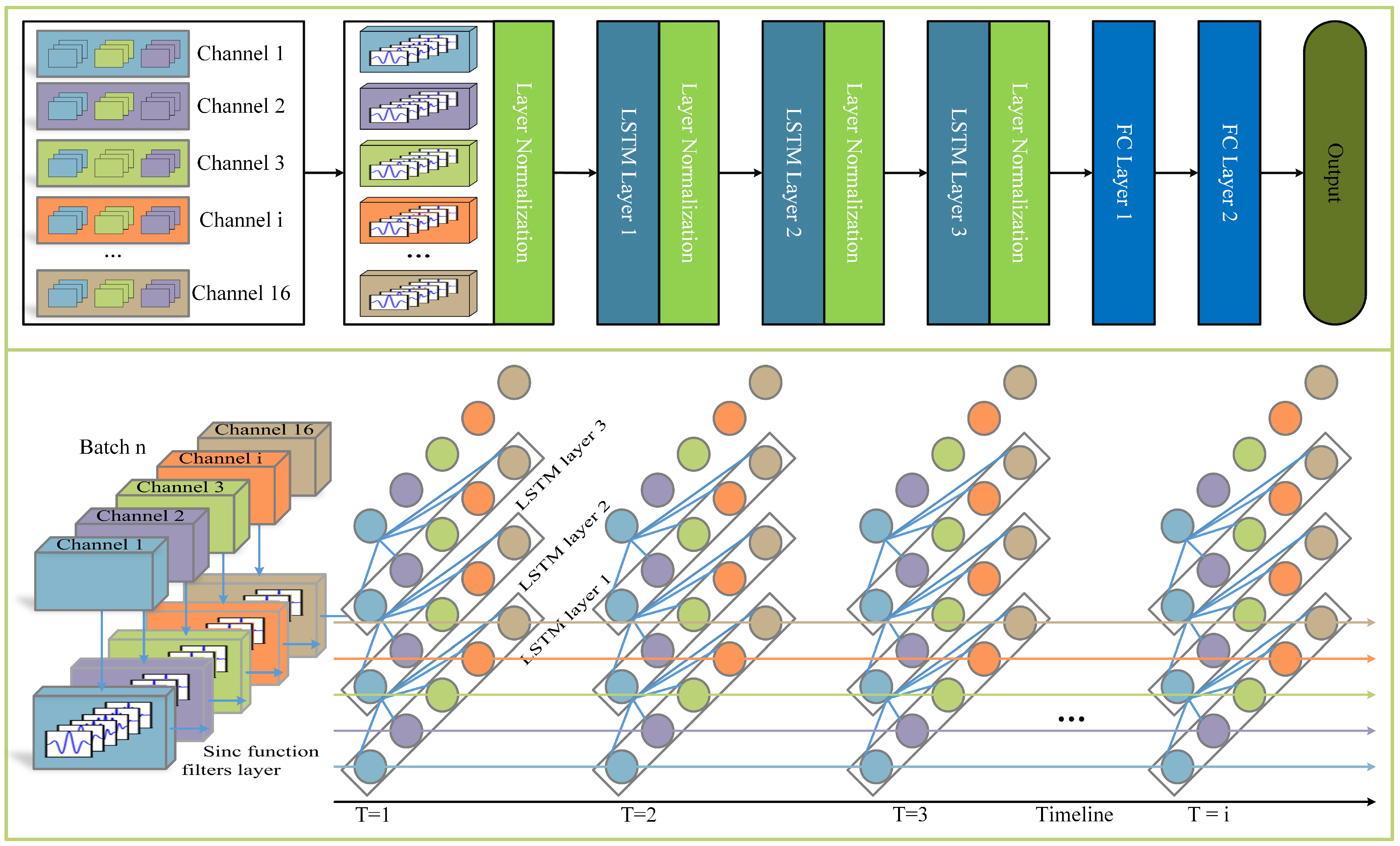
The structure of Sinc-LSTM network is shown in
Figure 2. Among them, the first layer of the hidden layer is composed of
Sinc function filters, and the LSTM network is composed of three LSTM one-way layers with 288 units. Layer normalization (LN) is applied to the Sinc filter layer and each LSTM layer to normalize their inputs and improve learning efficiency. The output of the LSTM flows through the dropout layer and the dense layer to prevent overfitting and is then output by the fully connected layer to complete the reconstruction of the sequence.
The various layers in the network are closely coordinated with each other and have their own functions. The SincNet layer is responsible for extracting local features from the input signal by convolving it with a bank of Sinc filters. The resulting feature sequence is then passed on to the LSTM layer, which is able to capture the temporal dependencies in the input sequence and learn long-term dependencies between different features. The output of the SincNet layer is fed into the LSTM layer as a sequence of feature vectors, which are processed in a recurrent manner. Overall, the SincNet layer and LSTM layer work together to extract and model both local and global features from the input sequence, allowing for more accurate and robust predictions. In addition, LN normalizes the inputs to each LSTM layer independently, reducing the internal covariate shift and improving the stability and efficiency of the learning process. Then before output, the dropout layer randomly removes a fraction of the neurons during training, which reduces overfitting by encouraging the network to learn more robust features. In the following paragraphs of this subsection, a detailed description of the structure and principles of each module will be provided.
Sinc function filter layer. Sinc function filters are obtained from SincNet networks. The structure of the Sinc function filter is shown in
Figure 3. SincNet was originally used to process speech signals. The shape of Sinc function filters is similar to the form of alternating peaks and troughs in 1D temporal data, thus providing a better fitting ability to 1D temporal data of speech signals. For time series, the standard CNN convolution formula is as in Equation (
4), where
is the speech signal,
is the filter of length
L, and
is the output of the filter. In the standard CNN structure, the
L elements of each filter are learned from the data. The Sinc function filter is defined as a filter
, whose frequency domain characteristics are shown in Equation (
5), where
and
are the low and high cutoff frequencies, respectively, which are learnable parameters in the filter.
The neural network regulates
and
by loss function so that the model can automatically adjust the band selected with the bandpass filter. Therefore, the model can extract more meaningful features and enhance the interpret ability of the network. As shown in
Figure 3, in the Sinc function filter layer of the hidden layer, we set six Sinc function filters with different initial cutoff frequencies for the 16 channel data of the CMG to extract the feature information of different frequency bands on each channel.
LSTM Network. The training and weight update visualization of the LSTM network is shown in
Figure 2, with each unit in each layer computing in parallel for each channel of the input. One update is performed at each time step until the individual channel data traversal is complete. The unit structure of the LSTM neural network is shown in
Figure 4. The LSTM network consists of multiple memory cells that allow the network to capture long-term dependencies in the input sequence. Each memory cell has a self-connected recurrent unit that maintains a hidden state and an input gate, output gate, and forget gate that regulate the flow of information into and out of the cell. The input gate controls the amount of new input that is added to the current hidden state, while the output gate determines how much of the cell’s current state is exposed to the rest of the network. The forget gate decides how much of the previous state should be forgotten.
The proposed LSTM network has three layers, with each layer comprising 288 LSTM cells. The output of each layer is fed as input to the next layer. The input to the network is a sequence of data points, and the output is a reconstructed sequence. LN modules are added to each LSTM layer to normalize the inputs to the next layer, reduce the effect of the vanishing gradient problem, and improve the stability and effectiveness of the network for processing sequential data.
A combination of dense layers and dropout layers are used after the LSTM layers to reduce overfitting and improve the generalization of the model. The network is trained by a variant of the backpropagation algorithm called the Adam optimizer, which is well-suited for training recurrent neural networks. To prevent overfitting and select the best-performing model based on validation accuracy, early stopping is also utilized. At last, full connection layers added to the sequence to sequence LSTM network can help to learn more complex mappings between sequences.
The proposed Sinc-LSTM network utilizes a sinc filter layer to extract relevant features from time series data, which are subsequently fed into the LSTM network for sequence modeling. By leveraging the feature extraction capabilities of SincNet with the temporal modeling capabilities of LSTM networks, the proposed approach enhanced the performance of CMG’s telemetry data time series anomaly detection. The Sinc-LSTM network obtains the mapping by training, and predicts and generates the l time steps of the reconstructed data according to the previous p time steps of the input data at the current time. The training set input for Sinc-LSTM training is organized as follows , where m is the number of reconstructed data channels and n is the length of reconstructed data.
The fitting reconstruction method is to model and analyze the data of each channel of the control torque gyroscope separately. The control moment gyroscope telemetry data were made into 16 data files, each containing the data from the remaining 15 channels as input and the data from a single channel as supervision. In the training process of the Sinc-LSTM network, the information of the remaining 15 channels is used as the input training data. After the training, the model parameters of the 16 channels are stored in different files.
3.4. Anomaly Detection
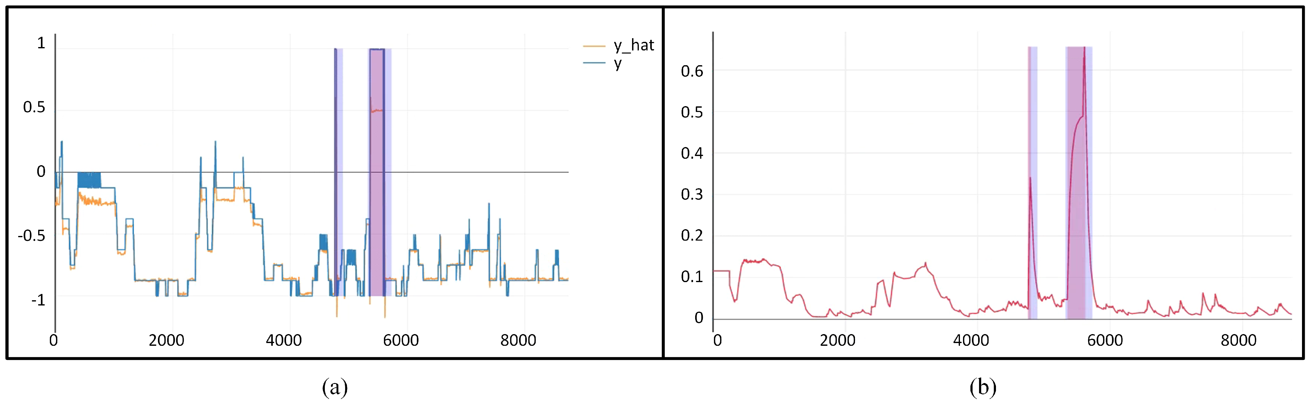
The image of the difference between the reconstructed data and the original data is shown in
Figure 5. When the difference result exceeds the threshold, it is judged as abnormal.
In the process of difference data calculation, the exponential weighted average method was used to smooth the difference sequence so as to avoid the noise generated by controlling torque gyroscope telemetry data mutation and other factors in the process of difference calculation being mistaken as abnormal, resulting in false positives and resulting in accuracy degradation.
At the same time, the setting of the threshold of the working condition segment is dynamic, and the setting of the threshold of each working condition segment is determined using the following formula:
where,
represents the abnormal judgment threshold of the ith working condition category,
represents the mean of the difference between the piecewise fitting reconstruction data and the original telemetry data of the working condition,
and
respectively represents the standard deviation of the piecewise difference and the standard deviation of the whole life cycle error of the working condition,
and
is a pair of constants set in advance, 5% and 20% respectively. Respectively, they represent the lowest acceptable anomaly detection threshold and the increase of anomaly detection threshold determined by the volatility of segmented data in the current working conditions.
4. Experiments
An anomaly detection dataset based on the full lifecycle data of CMGs on a spacecraft is produced for experimental validation of the proposed method. Existing spacecraft anomaly detection systems still rely mainly on manual evaluation. The dataset in the paper has been annotated with anomalies by qualified experts. CMG data were sampled every 10 days, for a total of 155 days of data. The CMG data is divided into 16 channels, including the gimbal motor current, rotor motor current, shaft temperature, speed, and other parameters. Since the data characteristics of each channel are different, the Sinc-LSTM network trains the anomaly detection task model separately for each channel data after pre-training. In the working condition classification stage, the data of each channel are first divided into hourly segments, and there are a total of segments. The data size of each segment after segmentation is about 16 channels and 6450 rows.
This section validates the effectiveness of each module of the proposed method and the advancement of the whole method, respectively, by setting up two sets of comparative experiments. The self-comparison experiments are conducted by ablating the work condition classification module, the migration learning method, and the SincNet filter layer of the model, and then comparing the experimental results to verify the contribution of each module to anomaly detection. The comparison experiments with state-of-the-art methods are conducted to verify the advancedness of the proposed method on the CMG dataset by comparing it with baseline and some of the latest anomaly detection methods.
4.1. Experimental Setup
The telemetry data are made into 16 data documents according to different channels. The first column of each data document is the sequence to be fitted and reconstructed, and the data of the remaining 15 channels follow. The Sinc-LSTM network is used to fit and reconstruct the first column of data in the data document.
The network setup is shown in
Figure 2. The main structure consists of one SincNet network and three LSTM networks. First, the data of the large-scale Mars orbiter MRO is input into the network for pre-training. The SincNet filter layer contains 96 Sinc filters and 288 LSTM units are configured for each of the three LSTM networks. Two fully connected layers were then set up. The three-layer LSTM network uses the hyperbolic tangent function as the activation function. Dropout is set in the network for regularization. Dropout is a regularization technique to avoid overfitting. It eliminates the joint adaptability of each unit in the neural network by randomly setting some units to 0, so as to enhance the generalization ability of the model. The Dropout ratio of the model was set to 0.3. The mean square error (MSE) was used as the loss function. The model parameters of Sinc-LSTM network are configured as shown in
Table 1. The same hyperparameter settings were used for all groups of experiments.
LSTM prediction requires setting the input sequence length p and output sequence length l. After adjustment, and were set. The initial learning rate was set to 0.001. The LSTM three-layer model has a shallow capacity, but it can provide sufficient model depth for each telemetry channel to be modeled separately. For each telemetry channel, the prediction reconstruction model is trained separately, and the segmented data are input into different batch networks according to the working condition category for training. Due to the poor parallelism of LSTM model training and the need to train 16 different models, the training time will be long. The two-stage transfer learning greatly reduces the time required for model convergence. Early stops are also set to reduce the overall training time. After testing, the model of each channel was set for training for 60 epochs, and the loss value was stopped in advance when it did not decline for 8 epochs.
Assuming that the point judged to be anomalous by the threshold is , the anomaly sequence corresponding to this anomaly is selected as . Selecting an anomaly sequence of a certain length can help the model perceive the sequence characteristics before the anomaly is generated and the impact on the telemetry data after the anomaly. There is also a need for a balance between computational accuracy and computational cost. When two anomaly sequences produce some overlap, they are determined to belong to the same anomaly event and are combined into a single anomaly sequence. The following criteria are used to determine the results of anomaly sequences.
True positive (TP): For the detected anomaly sequence , if any point of it falls in a true anomaly sequence , then the detected sequence is True positive.
False negative (FN): For the true anomaly sequences , if no point in the detected anomaly sequence falls within it, it is determined to be False negative.
False positive (FP): For the detected anomaly sequences , if there is no overlap with any true anomaly sequence, this detected anomaly sequence is False positive.
True negative (TN): For telemetry data time series , the points that are outside the true anomaly sequence and are not judged to be anomalies by the anomaly detection sequence are True negative.
The degree of overlap between the true anomaly sequence and the detected anomaly sequence is not included in the calculation of the evaluation of the anomaly detection results. The same method of locating anomaly sequences and the criteria for determining the detection results are used for all groups of experiments. The performance of the anomaly detection model can be evaluated with the help of four metrics: precision (
P), recall (
R), accuracy (
A), and an
score. The four metrics are calculated as follows:
P reflects the correctness of all detected anomalous sequences, and R reflects the degree to which anomaly detection results are found to be complete. These two metrics are of greater interest to anomaly detection tasks and are of greater reference value for practical engineering purposes. A reflects the correctness of the overall telemetry data classification task. The unbalanced data distribution is a significant feature of the anomaly detection task dataset, and therefore metric A is not a good indicator of the performance of the model. For example, for a 10% anomaly dataset, if the model determines that all data are normal, A is still 90%, while P, R, and scores are all 0. Therefore, A for the anomaly detection task can be used as a secondary reference metric but not the primary basis for judging model performance. The score is a harmonized average of P and R, and reflects the overall performance of the anomaly detection model by taking into account both the precision and recall of the model.
4.2. Self Contrast Experiments
In order to verify the effectiveness of each step of the proposed method, self-comparison experiments are set up. One step of the proposed method is omitted at a time, and then the experimental results are compared with those of the complete method. In this subsection, we will first introduce the treatment method after each step is deleted, and then show the experimental results.
First, the experimental group with the working condition classification step was deleted. In the working condition classification stage, each telemetry channel is segmented and clustered separately, and then the telemetry data file is made according to the clustering results of the channel to be predicted. After the telemetry data files are made, they are divided into different batches according to different working conditions to input into the network for piecewise reconstruction of telemetry data. After deleting the condition classification step, the data of the whole period is segmented without clustering and directly input into the network for training. At the same time, a constant threshold is set for anomaly detection based on the full-period data. After canceling the adaptive threshold judgment of the working condition classification, the abnormal false detection rate will be greatly increased because the threshold is not adaptive to each working condition stage.
Then is the experimental group with deletion of transfer learning step. This step contains two control groups. One group is the result of no pre-training, and the initial weight of the network is randomly generated, and the other group is the result of one-stage pre-training using only the MRO dataset. The experimental group without pre-training will greatly decrease the convergence speed during the training of the CMG, so the maximum number of training times is set to 100 epochs. In the control group without transfer learning pre-training, the generalization ability will be greatly reduced in addition to the training speed. Due to the characteristics of fault data, it is difficult to obtain the annotated fault data. The model does not converge easily due to the small size of the CMG dataset, and too many iterations tend to cause overfitting. It is beneficial to reduce the overfitting of the network and enhance the generalization ability of the model by extracting the universal features of the spacecraft time series data into the network by pre-training. The precision and recall of anomaly detection in the control group with deletion of the transfer learning step will be greatly reduced. One stage of transfer learning can greatly improve the performance of the network.
Finally, the experimental group with the Sinc function filter layer was deleted. Sinc function filter can well fit the characteristics of one-dimensional temporal data due to its interpretability and special band-pass filter structure. Setting the Sinc filter layer at the input end of the network is helpful in improving the feature extraction ability of the network for one-dimensional temporal data. In this paper, six Sinc filters with different bandwidths are set to extract features from the network. In the training process, the number of parameters can be reduced, and the training efficiency can also be improved. The ability of network fitting to reconstruct time series data with the deletion of the Sinc filter layer is affected. The accuracy of the tests and the recall rate have decreased.
Experimental results and analysis. Experimental renderings are shown in
Figure 5, with original data and reconstructed sequences on the left and difference sequences and detected abnormal sequences on the right. Abnormal detection results are shown in
Table 2. It can be seen that the precision and recall rate of the proposed method have reached the highest. In the control group, the performance of the control group with the deletion of transfer learning step decreased the most, the accuracy and recall decreased by 22.2% and 19.9%, respectively. The control group with one-stage transfer learning had the least performance degradation, with accuracy and recall decreasing by 2.2% and 1.5%, respectively. It can be seen that all the steps proposed in this paper have improved the performance of the anomaly detection model. Among them, transfer learning and training steps have the highest performance improvement. The training times for each experimental group are shown in
Table 2. It can be seen that the average convergence time is much shorter for the pre-trained experimental groups. The addition of the Sinc function filter layer, although adding an additional layer to the network, did not have a significant impact on the training time as it better extracted the features of the 1D signal and facilitated the convergence of the model.
4.3. Compared with Advanced Methods
Hundman et al. [
14] provide the telemetry dataset of SMAP&MSL and propose an anomaly detection method using LSTM and non-parametric dynamic threshold. Reference work [
49] verifies that the method of generating adversarial networks can be used for unsupervised anomaly detection, and adopts LSTM network structure and cyclic consistency loss training. The SVM method proposed in [
50] also improves the anomaly detection of LSTM. This section compares the proposed method with these advanced anomaly detection methods.
The anomaly detection results are shown in
Figure 5. In
Figure 5a, Y and y_hat represent the original data and reconstructed sequences, respectively, and the abnormal sequences are marked. In
Figure 5b, the red line represents the smoothed result of the difference between the original data and the reconstructed sequence, and marks the anomaly detection result judged by the threshold. The anomaly detection effects of different methods are shown in
Table 3. The different methods are all simple parameter debugging. Due to the small capacity of the CMG anomaly detection dataset, the network models adopted using the advanced methods in comparison have used the MRO dataset for a stage of pre-training. At the same time, the learning rate and dropout are adjusted to be consistent with the proposed method.
It can be seen from
Table 3 that the proposed method is superior to other methods in CMG telemetry data anomaly detection task.
5. Conclusions
This article proposes a CMG anomaly detection method based on working condition classification and transfer learning. A two-stage transfer learning is designed to solve the problem of poor training effect due to the lack of fault data. A Sinc-LSTM network is designed to model each telemetry channel separately, classify the working conditions and set adaptive thresholds for anomaly detection. Experimental results show that transfer learning, working condition classification, and a Sinc filtering layer can improve the performance of CMG anomaly detection tasks, with the improvement of transfer learning being the most significant. Working condition classification is a refined processing method for anomaly detection in long-cycle tasks and is also of great significance. As a key inertial execution component, the operational data of the CMG is representative, and the anomaly detection method for the CMG can also be transferred to other parts of the spacecraft. In addition, by adjusting the training set, the proposed method can be applied to other time-series data anomaly detection tasks.
During the training process, the model still has shortcomings, such as slow convergence speed and low training efficiency. Faced with thousands of telemetry data channels commonly used in spacecraft, the time cost of the strategy proposed for training each channel separately is high. To address the problem of large-scale telemetry data and multiple channels in spacecraft, a universal model for spacecraft component anomaly detection with strong generalization ability can be trained by increasing the depth of the model and the size of the training set. Introducing the time-frequency two-dimensional features of one-dimensional signals can enhance the neural network’s perception of nonlinear time-varying features. Moreover, using models without temporal dependencies, such as convolutional neural networks, can greatly reduce the time cost of model training. In the future, our research will be based on deep learning, transfer learning, time-frequency analysis, and other methods, involving fault diagnosis of spacecraft multimodal signals and complex systems.


