
Enhancing Ductal Carcinoma Classification Using Transfer Learning with 3D U-Net Models in Breast Cancer Imaging


 , , , and
Abstract
:1. Introduction
1.1. Background
1.2. Motivation
1.3. Research Question
- (a)
- Explore the impact of different pre-training datasets and hyperparameter settings on the performance of transfer learning with 3D U-Net models, as well as its potential application in the detection and diagnosis of other types of breast cancer and medical imaging applications.
- (b)
- Consider the potential challenges and opportunities associated with integrating transfer learning with 3D U-Net models into existing clinical workflows for breast cancer imaging and computer-aided diagnosis.
1.4. Research Design
- (a)
- This study explores the potential of transfer learning in enhancing the classification of ductal carcinoma using 3D U-Net models in breast cancer imaging.
- (b)
- To overcome the issue of limited annotated data, this research investigates the effectiveness of fine-tuning a pre-trained 3D U-Net model on a publicly accessible dataset for breast cancer imaging.
- (c)
- The evaluation of the fine-tuned 3D U-Net model on a separate testing dataset, demonstrating the effectiveness of transfer learning in improving the accuracy of ductal carcinoma classification.
- (d)
- The demonstration of the potential for the proposed approach to serve as a valuable tool for radiologists and medical practitioners in the computer-aided diagnosis and treatment of cancers.
2. Related Work
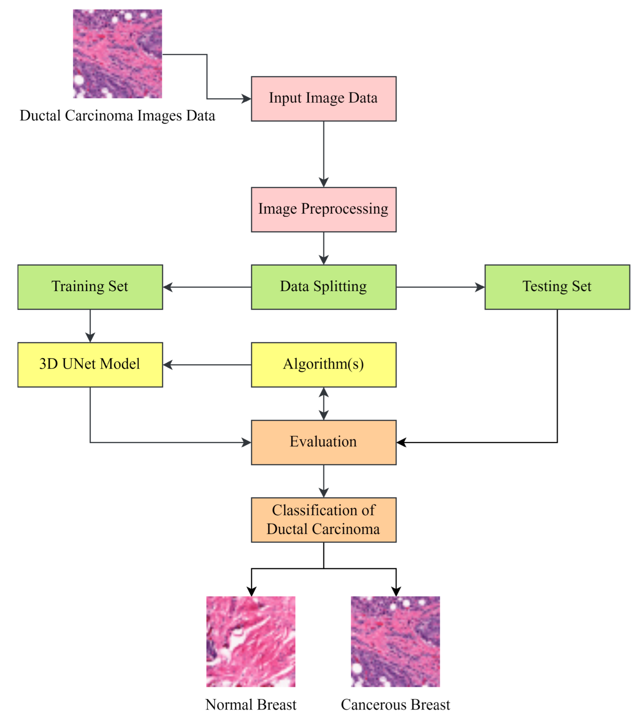
3. Methodology
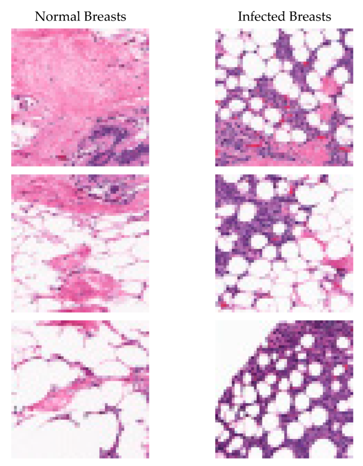
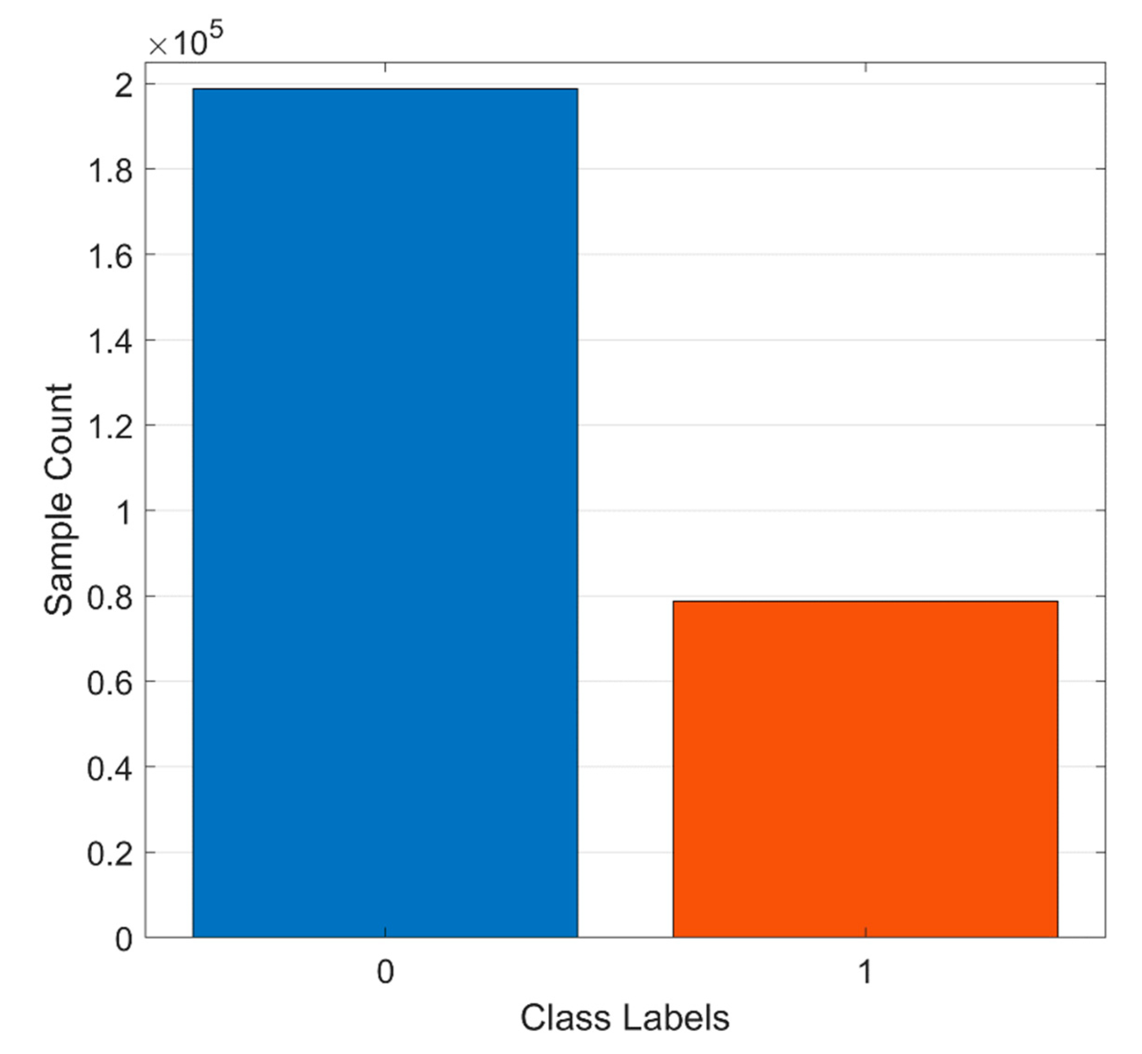
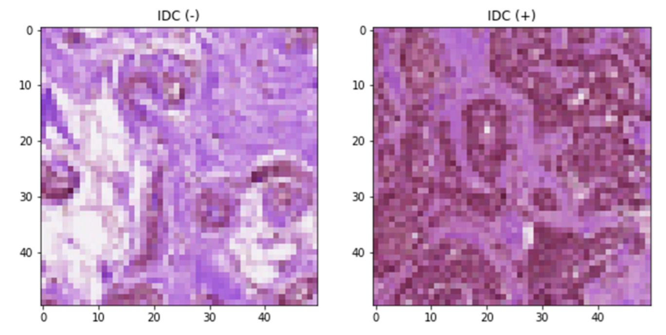
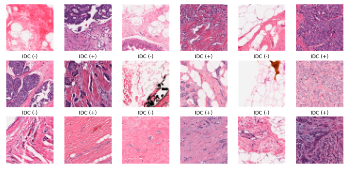
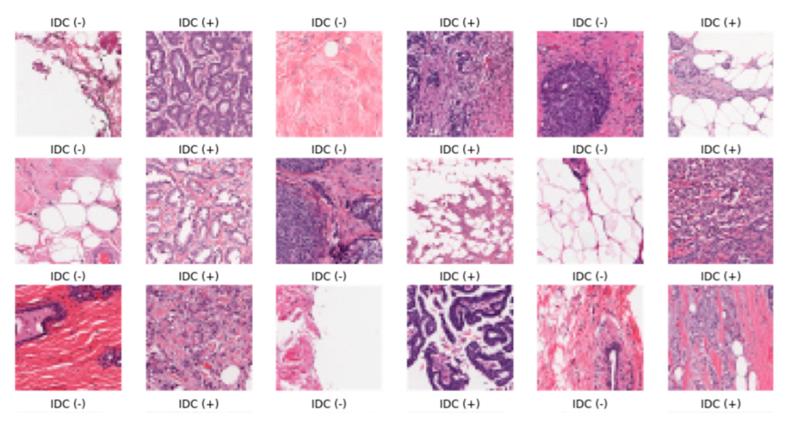
3.1. Dataset Description
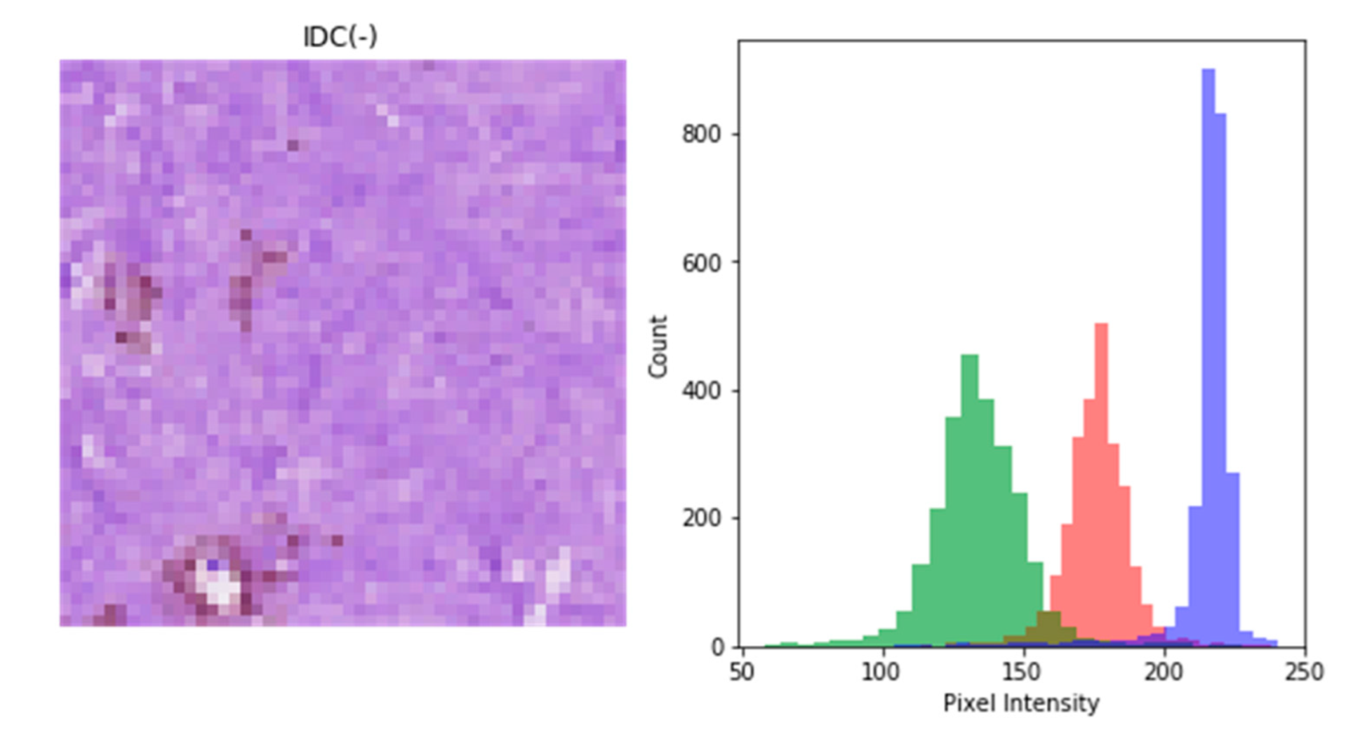
3.2. Image Preprocessing
3.2.1. Resizing
- Nearest neighbor interpolation:
- Bilinear interpolation:
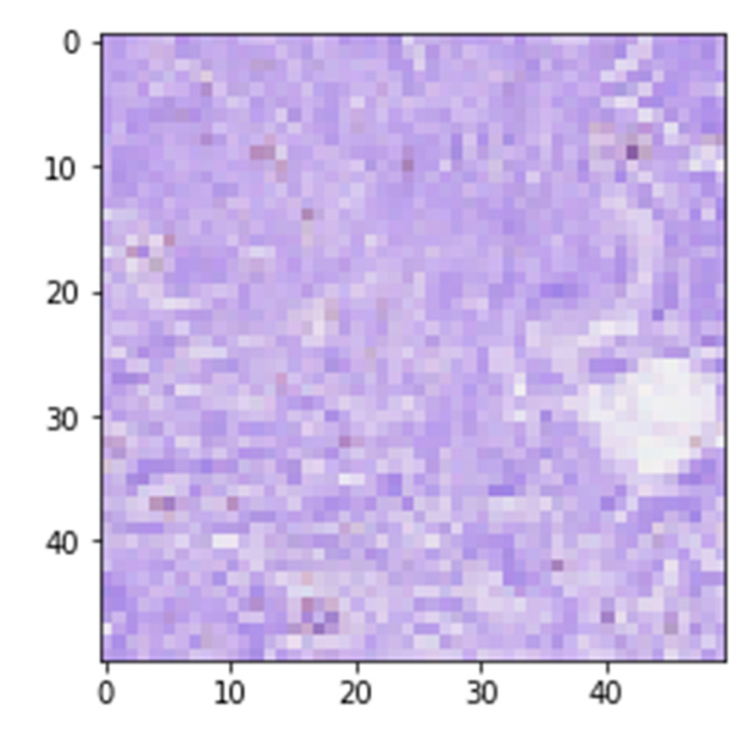
3.2.2. Intensity Normalization
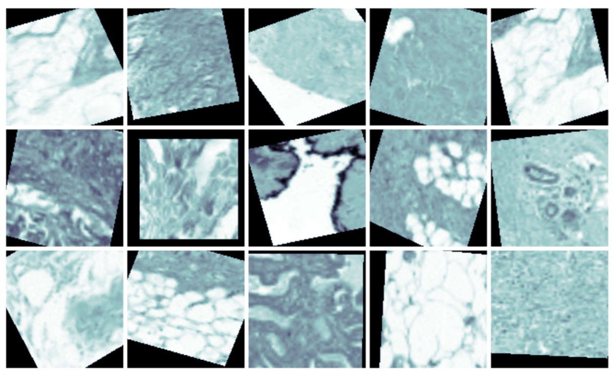
3.2.3. Data Augmentation
- a
- Rotation:
- b
- Flipping:
- c
- Scaling:
- d
- Translation:
3.2.4. Extraction of Patches
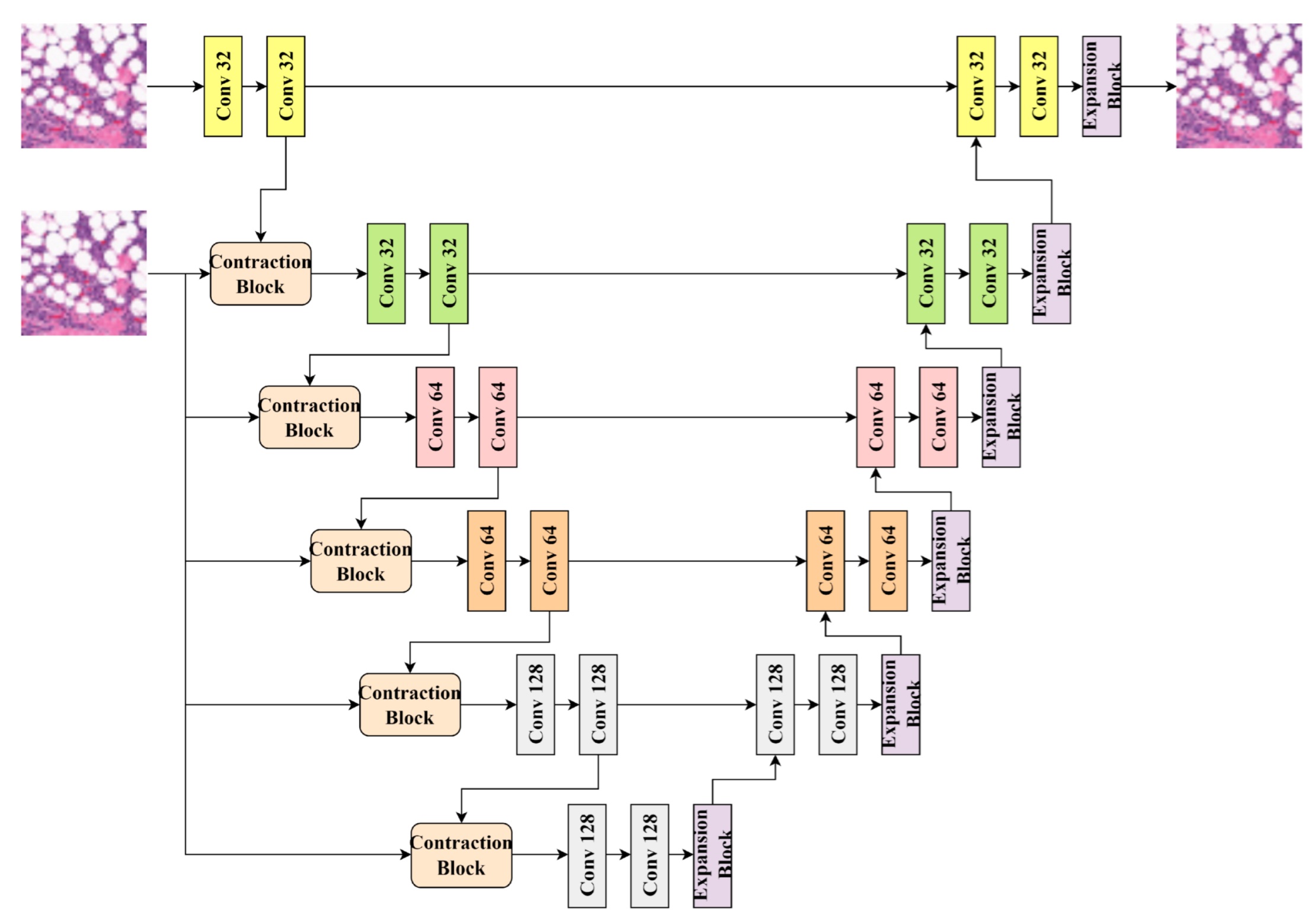
3.3. D U-Net Model for Classification
- Convolution:
- Max Pooling:
- Up-sampling:
- Transposed Convolution:
3.4. Fine-Tuning of 3D U-Nets
- Loss Function:
- Optimization Algorithm:
- Regularization:
3.5. Performance Evaluation
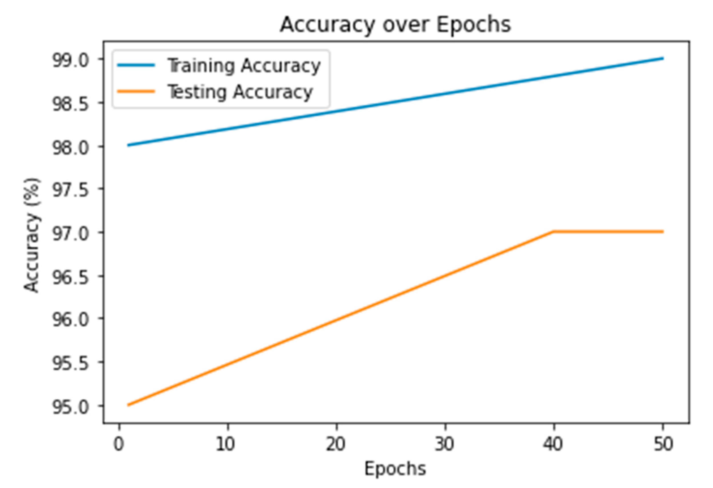
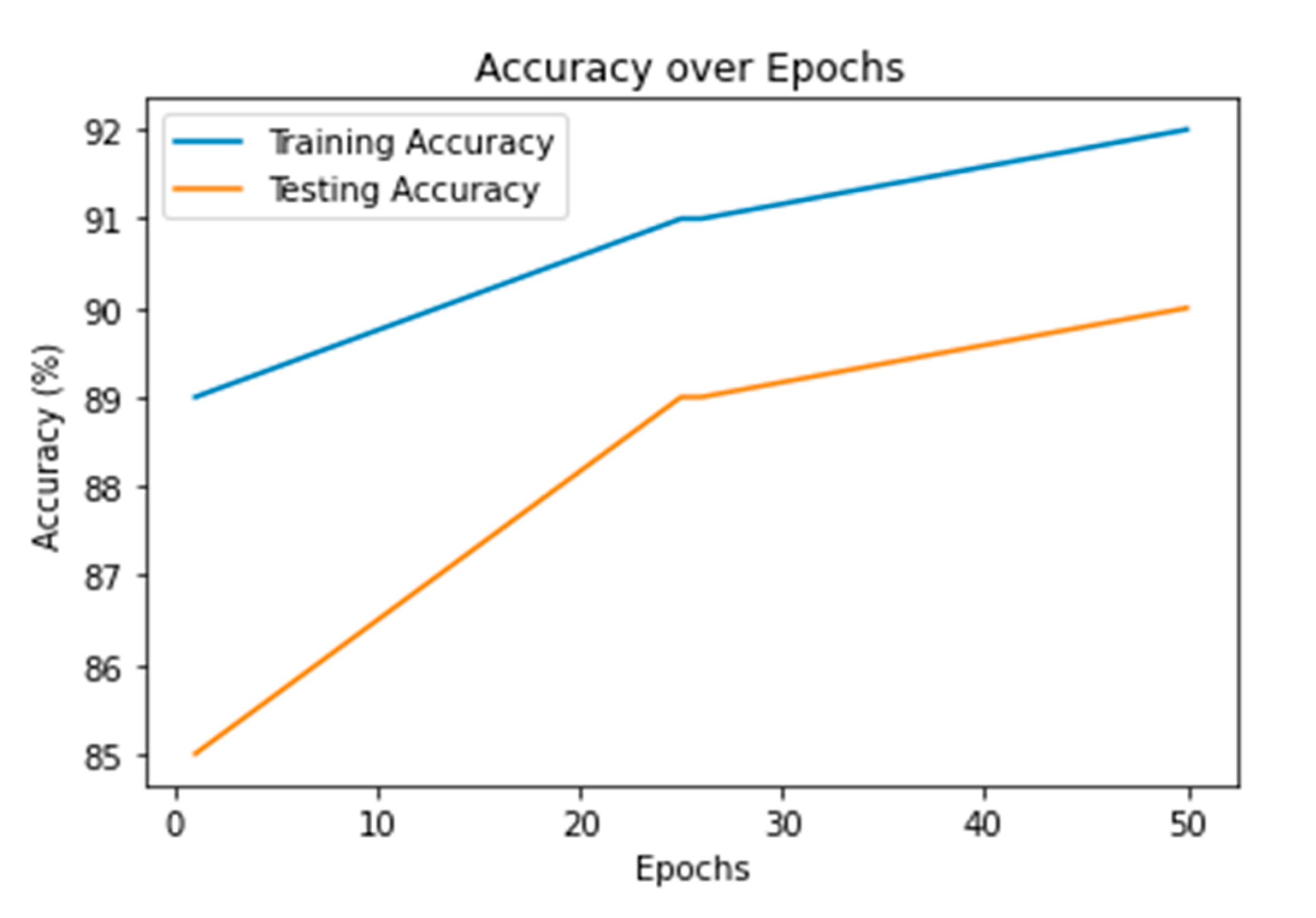
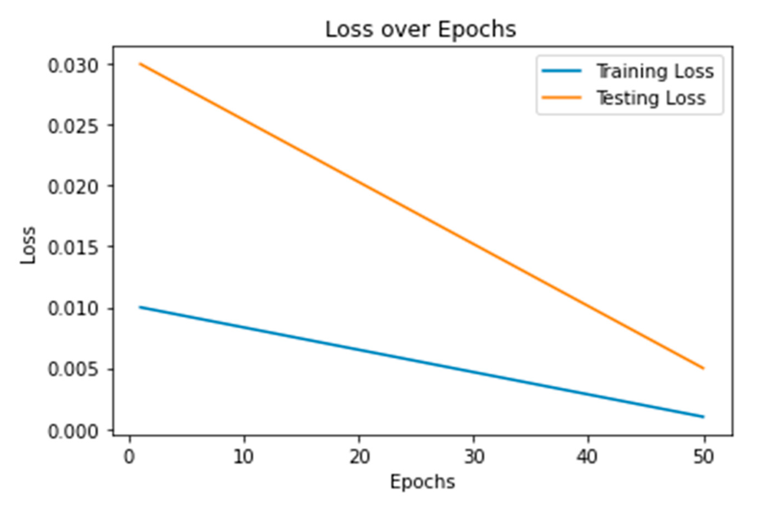
- Training and Testing Accuracy:
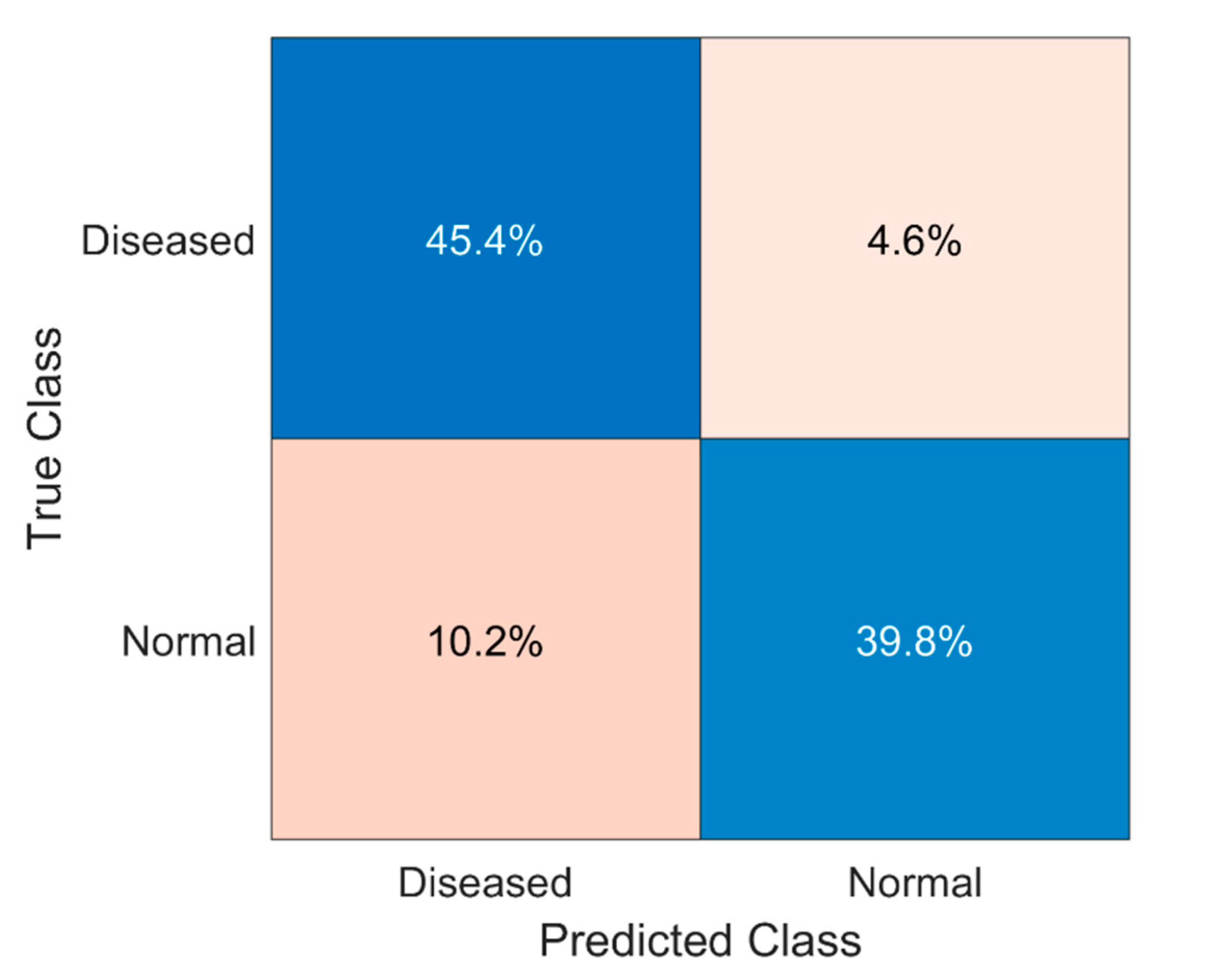
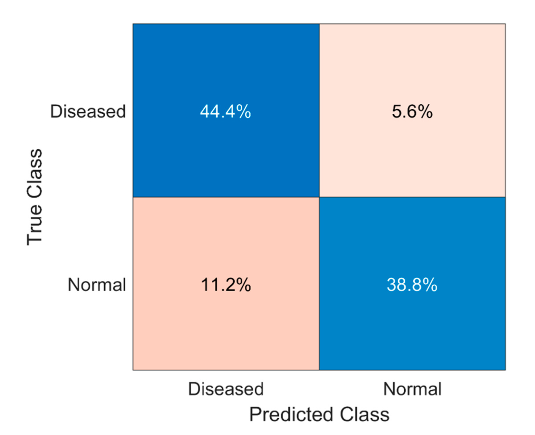
- Confusion Matrix:
4. Results & Discussion
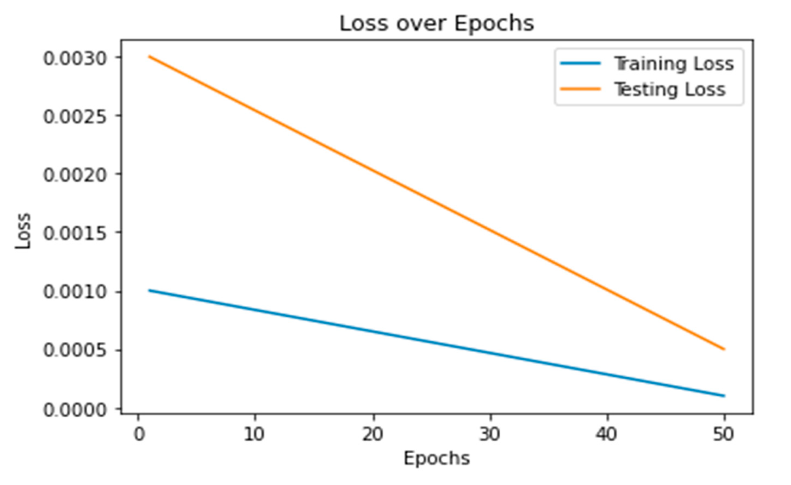
4.1. Performance of Fine-Tuned 3D U-Net Model
4.2. Performance of Simple 3D U-Net Model
5. Conclusions
Author Contributions
Funding
Data Availability Statement
Acknowledgments
Conflicts of Interest
References
- Carter, E.P.; Gopsill, J.A.; Gomm, J.J.; Jones, J.L.; Grose, R.P. A 3D in vitro model of the human breast duct: A method to unravel myoepithelial-luminal interactions in the progression of breast cancer. Breast Cancer Res. 2017, 19, 1–10. [Google Scholar] [CrossRef] [PubMed] [Green Version]
- Ghani, M.U.; Alam, T.M.; Jaskani, F.H. Comparison of Classification Models for Early Prediction of Breast Cancer. In Proceedings of the 2019 International Conference on Innovative Computing (ICIC), Lahore, Pakistan, 1–2 November 2019. [Google Scholar] [CrossRef]
- Dafni, U.; Tsourti, Z.; Alatsathianos, I. Breast cancer statistics in the european union: Incidence and survival across european countries. Breast Care 2019, 14, 344–353. [Google Scholar] [CrossRef] [PubMed]
- Wolfe, J.N. Breast Patterns as Index of Breast. AJR Am. J. Roentgenol. 1976, 126, 1130–1139. [Google Scholar] [CrossRef] [PubMed]
- Brunetti, A.; Carnimeo, L.; Trotta, G.F.; Bevilacqua, V. Computer-assisted frameworks for classification of liver, breast and blood neoplasias via neural networks: A survey based on medical images. Neurocomputing 2019, 335, 274–298. [Google Scholar] [CrossRef]
- Ghias, A.F.; Epps, G.; Cottrill, E.; Mardekian, S.K. Multifocal Metastatic Breast Carcinoma to the Thyroid Gland Histologically Mimicking C Cell Lesions. Case Rep. Pathol. 2019, 2019, 1–5. [Google Scholar] [CrossRef]
- Caumo, F.; Bernardi, D.; Ciatto, S.; Macaskill, P.; Pellegrini, M.; Brunelli, S.; Tuttobene, P.; Bricolo, P.; Fantò, C.; Valentini, M.; et al. Incremental effect from integrating 3D-mammography (tomosynthesis) with 2D-mammography: Increased breast cancer detection evident for screening centres in a population-based trial. Breast 2014, 23, 76–80. [Google Scholar] [CrossRef]
- Bhattacharjee, R.; Douglas, L.; Drukker, K.; Hu, Q.; Fuhrman, J.; Sheth, D.; Giger, M.L. Comparison of 2D and 3D U-Net breast lesion segmentations on DCE-MRI. In Proceedings of the Proceedings Volume 11597, Medical Imaging 2021: Computer-Aided Diagnosis, Online, 15–20 February 2021; p. 10. [Google Scholar] [CrossRef]
- Anand, I.; Negi, H.; Kumar, D.; Mittal, M.; Kim, T.H.; Roy, S. Residual U-Network for Breast Tumor Segmentation from Magnetic Resonance Images. Comput. Mater. Contin. 2021, 67, 3107–3127. [Google Scholar] [CrossRef]
- Mirza, A.; Abdulsalam, F.; Asif, R.; Dama, Y.; Abusitta, M.; Elmegri, F.; Abd-Alhameed, R.; Noras, J.; Qahwaji, R. Breast cancer detection using 1D, 2D and 3D FDTD numerical methods. In Proceedings of the 2015 IEEE International Conference on Computer and Information Technology; Ubiquitous Computing and Communications; Dependable, Autonomic and Secure Computing; Pervasive Intelligence and Computing, Liverpool, UK, 26–28 October 2015; pp. 1042–1045. [Google Scholar] [CrossRef]
- Wang, L.; Simpkin, R.; Al-Jumaily, A.M. 3D breast cancer imaging using holographic microwave interferometry. In Proceedings of the IVCNZ′12: Proceedings of the 27th Conference on Image and Vision Computing New Zealand, Dunedin New Zealand, 26–28 November 2012; pp. 180–185. [CrossRef]
- Vidavsky, N.; Kunitake, J.A.M.R.; Diaz-Rubio, M.E.; Chiou, A.E.; Loh, H.-C.; Zhang, S.; Masic, A.; Fischbach, C.; Estroff, L.A. Mapping and Profiling Lipid Distribution in a 3D Model of Breast Cancer Progression. ACS Cent. Sci. 2019, 5, 768–780. [Google Scholar] [CrossRef] [Green Version]
- Zhuang, Z.; Li, N.; Raj, A.N.J.; Mahesh, V.G.V.; Qiu, S. An RDAU-NET model for lesion segmentation in breast ultrasound images. PLoS ONE 2019, 14, e0221535. [Google Scholar] [CrossRef] [Green Version]
- Gardezi, S.J.S.; Elazab, A.; Lei, B.; Wang, T. Breast cancer detection and diagnosis using mammographic data: Systematic review. J. Med. Internet Res. 2019, 21, 1–22. [Google Scholar] [CrossRef] [Green Version]
- Ciatto, S.; Houssami, N.; Bernardi, D.; Caumo, F.; Pellegrini, M.; Brunelli, S.; Tuttobene, P.; Bricolo, P.; Fantò, C.; Valentini, M.; et al. Integration of 3D digital mammography with tomosynthesis for population breast-cancer screening (STORM): A prospective comparison study. Lancet Oncol. 2013, 14, 583–589. [Google Scholar] [CrossRef] [PubMed]
- Nayankumar, P.H. Microwave Imaging for Breast Cancer Detection using 3D Level Set based Optimization, FDTD Method and Method of Moments. Ph.D. Thesis, Dhirubhai Ambani Institute of Information and Communication Technology, Gujarat, India, 2019. [Google Scholar]
- Halim, A.A.A.; Andrew, A.M.; Yasin, M.N.M.; Rahman, M.A.A.; Jusoh, M.; Veeraperumal, V.; A Rahim, H.; Illahi, U.; Karim, M.K.A.; Scavino, E. Existing and emerging breast cancer detection technologies and its challenges: A review. Appl. Sci. 2021, 11, 10753. [Google Scholar] [CrossRef]
- Zebari, D.A.; Ibrahim, D.A.; Zeebaree, D.Q.; Mohammed, M.A.; Haron, H.; Zebari, N.A.; Damaševičius, R.; Maskeliūnas, R. Breast Cancer Detection Using Mammogram Images with Improved Multi-Fractal Dimension Approach and Feature Fusion. Appl. Sci. 2021, 11, 12122. [Google Scholar] [CrossRef]
- Balkenende, L.; Teuwen, J.; Mann, R.M. Application of Deep Learning in Breast Cancer Imaging. Semin. Nucl. Med. 2022, 52, 584–596. [Google Scholar] [CrossRef] [PubMed]
- Bae, M.S.; Kim, H.G. Breast cancer risk prediction using deep learning. Radiology 2021, 301, 559–560. [Google Scholar] [CrossRef] [PubMed]
- Govinda, E.; Ph, D.; Pradesh, A. Breast Cancer Detection Using UWB Imaging and Convolutional Neural Network. Ilkogr. Online 2021, 20, 1657–1670. [Google Scholar] [CrossRef]
- Nassif, A.B.; Talib, M.A.; Nasir, Q.; Afadar, Y.; Elgendy, O. Breast cancer detection using artificial intelligence techniques: A systematic literature review. Artif. Intell. Med. 2022, 127, 102276. [Google Scholar] [CrossRef]
- Sugimoto, M.; Hikichi, S.; Takada, M.; Toi, M. Machine learning techniques for breast cancer diagnosis and treatment: A narrative review. Ann. Breast Surg. 2023, 7, 7. [Google Scholar] [CrossRef]
- Durai, S.G.; Ganesh, S.H.; Christy, A.J. Prediction of breast cancer through classification algorithms: A survey. Int. J. Control Theory Appl. 2016, 9, 359–365. [Google Scholar]
- Sangari, N.; Qu, Y. A Comparative Study on Machine Learning Algorithms for Predicting Breast Cancer Prognosis in Improving Clinical Trials. In Proceedings of the 2020 International Conference on Computational Science and Computational Intelligence (CSCI), Las Vegas, NV, USA, 16–18 December 2020; pp. 813–818. [Google Scholar] [CrossRef]
- Al-Shargabi, B.; Al-Shami, F. An experimental study for breast cancer prediction algorithms. In Proceedings of the DATA’19: Proceedings of the Second International Conference on Data Science, E-Learning and Information Systems, Dubai, United Arab Emirates, 2–5 December 2019; pp. 3–8. [Google Scholar] [CrossRef]
- Dehdar, S.; Salimifard, K.; Mohammadi, R.; Marzban, M.; Saadatmand, S.; Fararouei, M.; Dianati-Nasab, M. Applications of different machine learning approaches in prediction of breast cancer diagnosis delay. Front. Oncol. 2023, 13, 1103369. [Google Scholar] [CrossRef]
- Wang, L. Microwave Sensors for Breast Cancer Detection. Sensors 2018, 18, 655. [Google Scholar] [CrossRef] [PubMed] [Green Version]
- Balasubramanian, S. Breast Cancer Prediction Using Machine Learning. Master’s Thesis, Department of Computer Science and Information System, California State University San Marcos, San Marcos, CA, USA, 2021. [Google Scholar]
- Asri, H.; Mousannif, H.; Al Moatassime, H.; Noel, T. Using Machine Learning Algorithms for Breast Cancer Risk Prediction and Diagnosis. Procedia Comput. Sci. 2016, 83, 1064–1069. [Google Scholar] [CrossRef] [Green Version]
- Islam, M.M.; Haque, M.R.; Iqbal, H.; Hasan, M.M.; Hasan, M.; Kabir, M.N. Breast Cancer Prediction: A Comparative Study Using Machine Learning Techniques. SN Comput. Sci. 2020, 1, 1–14. [Google Scholar] [CrossRef]
- Shakkeera, L.; Pandey, R.R.; Bhardwaj, R.; Singh, S.V.; Mukherjee, S.S. Analysis and Prediction of Breast Cancer using Machine Learning Techniques. Int. J. Eng. Adv. Technol. 2020, 10, 26–30. [Google Scholar] [CrossRef]
- Baghdadi, N.A.; Malki, A.; Balaha, H.M.; Badawy, M.; Elhosseini, M. Classification of breast cancer using a manta-ray foraging optimized transfer learning framework. PeerJ Comput. Sci. 2022, 8, 1054. [Google Scholar] [CrossRef] [PubMed]
- Madani, M.; Behzadi, M.M.; Nabavi, S. The Role of Deep Learning in Advancing Breast Cancer Detection Using Different Imaging Modalities: A Systematic Review. Cancers 2022, 14, 5334. [Google Scholar] [CrossRef] [PubMed]
- Pathan, R.K.; Alam, F.I.; Yasmin, S.; Hamd, Z.Y.; Aljuaid, H.; Khandaker, M.U.; Lau, S.L. Breast Cancer Classification by Using Multi-Headed Convolutional Neural Network Modeling. Healthcare 2022, 10, 2367. [Google Scholar] [CrossRef]
- Khamparia, A.; Bharati, S.; Podder, P.; Gupta, D. Diagnosis of breast cancer based on modern mammography using hybrid transfer learning. Multidimens. Syst. Signal Process. 2021, 32, 747–765. [Google Scholar] [CrossRef]
- Ahmed, B.E.N. Hybrid UNET Model Segmentation for an Early Breast Cancer Detection using Ulrasound Images. In Computational Collective Intelligence, Proceedings of the 14th International Conference, ICCCI 2022, Hammamet, Tunisia, 28–30 September 2022; Springer International Publishing: Cham, Switzerland, 2022; pp. 464–476. [Google Scholar] [CrossRef]
- Sailasya, G.; Kumari, G.L.A. Analyzing the Performance of Stroke Prediction using ML Classification Algorithms. Int. J. Adv. Comput. Sci. Appl. 2021, 12, 539–545. [Google Scholar] [CrossRef]
- Choi, Y.; Choi, J.W. Stroke Prediction Using Machine Learning based on Artificial Intelligence. Int. J. Adv. Trends Comput. Sci. Eng. 2020, 9, 8916–8921. [Google Scholar] [CrossRef]
- Yarabarla, M.S.; Ravi, L.K.; Sivasangari, A. Breast cancer prediction via machine learning. In Proceedings of the 2019 3rd international conference on trends in electronics and informatics (ICOEI), Tirunelveli, India, 23–25 April 2019; pp. 121–124. [Google Scholar] [CrossRef]
- Obayya, M.; Maashi, M.S.; Nemri, N.; Mohsen, H.; Motwakel, A.; Osman, A.E.; Alneil, A.A.; Alsaid, M.I. Hyperparameter Optimizer with Deep Learning-Based Decision-Support Systems for Histopathological Breast Cancer Diagnosis. Cancers 2023, 15, 885. [Google Scholar] [CrossRef] [PubMed]


| References | Datasets | Techniques | Results |
|---|---|---|---|
| Sugimoto et al. [23] | Cancer Imaging Archive (TCIA) | Fine-tuning | Improved ductal carcinoma classification using fine-tuned 3D U-NET model. |
| Al-Shargabi et al. [26] | Digital Database for Screening Mammography (DDSM) | Feature Extraction | Feature extraction from 3D U-NET improves carcinoma classification. |
| Islam et al. [31] | IN-breast | Multi-task learning | Multi-task 3D U-NET improves both carcinoma classification and segmentation. |
| Khamparia et al. [36] | Breast Cancer Histopathological Image | Unsupervised domain adaptation | Unsupervised adaptation of 3D U-NET improves carcinoma classification. |
| Reference | Dataset | Model | Accuracy |
|---|---|---|---|
| Obayya et al. [41] | Histopathological data of breasts | AOADL-HBCC | 95% |
| Sugimoto et al. [23] | Histopathological data of breasts | CNN | 91.5% |
| Vidavsky et al. [12] | Histopathological data of breasts | AlexNet | 90% |
| Bhattacharjee et al. [8] | Histopathological data of breasts | ResNet | 89% |
| This study | Histopathological data of breasts | 3D U-Net | 97% |
Disclaimer/Publisher’s Note: The statements, opinions and data contained in all publications are solely those of the individual author(s) and contributor(s) and not of MDPI and/or the editor(s). MDPI and/or the editor(s) disclaim responsibility for any injury to people or property resulting from any ideas, methods, instructions or products referred to in the content. |
© 2023 by the authors. Licensee MDPI, Basel, Switzerland. This article is an open access article distributed under the terms and conditions of the Creative Commons Attribution (CC BY) license (https://creativecommons.org/licenses/by/4.0/).
Share and Cite
Khalil, S.; Nawaz, U.; Zubariah; Mushtaq, Z.; Arif, S.; ur Rehman, M.Z.; Qureshi, M.F.; Malik, A.; Aleid, A.; Alhussaini, K. Enhancing Ductal Carcinoma Classification Using Transfer Learning with 3D U-Net Models in Breast Cancer Imaging. Appl. Sci. 2023, 13, 4255. https://doi.org/10.3390/app13074255
Khalil S, Nawaz U, Zubariah, Mushtaq Z, Arif S, ur Rehman MZ, Qureshi MF, Malik A, Aleid A, Alhussaini K. Enhancing Ductal Carcinoma Classification Using Transfer Learning with 3D U-Net Models in Breast Cancer Imaging. Applied Sciences. 2023; 13(7):4255. https://doi.org/10.3390/app13074255
Chicago/Turabian StyleKhalil, Saman, Uroosa Nawaz, Zubariah, Zohaib Mushtaq, Saad Arif, Muhammad Zia ur Rehman, Muhammad Farrukh Qureshi, Abdul Malik, Adham Aleid, and Khalid Alhussaini. 2023. "Enhancing Ductal Carcinoma Classification Using Transfer Learning with 3D U-Net Models in Breast Cancer Imaging" Applied Sciences 13, no. 7: 4255. https://doi.org/10.3390/app13074255