

Modeling Power Flows and Electromagnetic Fields Induced by Compact Overhead Lines Feeding Traction Substations of Mainline Railroads


Abstract
:1. Introduction
- We propose original models of power systems and power supply systems for AC railroads, with such models enabling quantitative evaluation of efficacy and the application of COHLs for supplying power to traction substations;
- The approach adopted for the creation of these models stands apart from other approaches in that it is system-based and treats COHLs as inseparable from the power flows of a complex power system.
- In contrast to traditional methods based on a single-line representation, our models were built using the three-phase (ABC) reference frame, which provides the most adequate modeling of power system load flows with single-phase traction loads that create significant imbalances in the electrical networks that feed them.
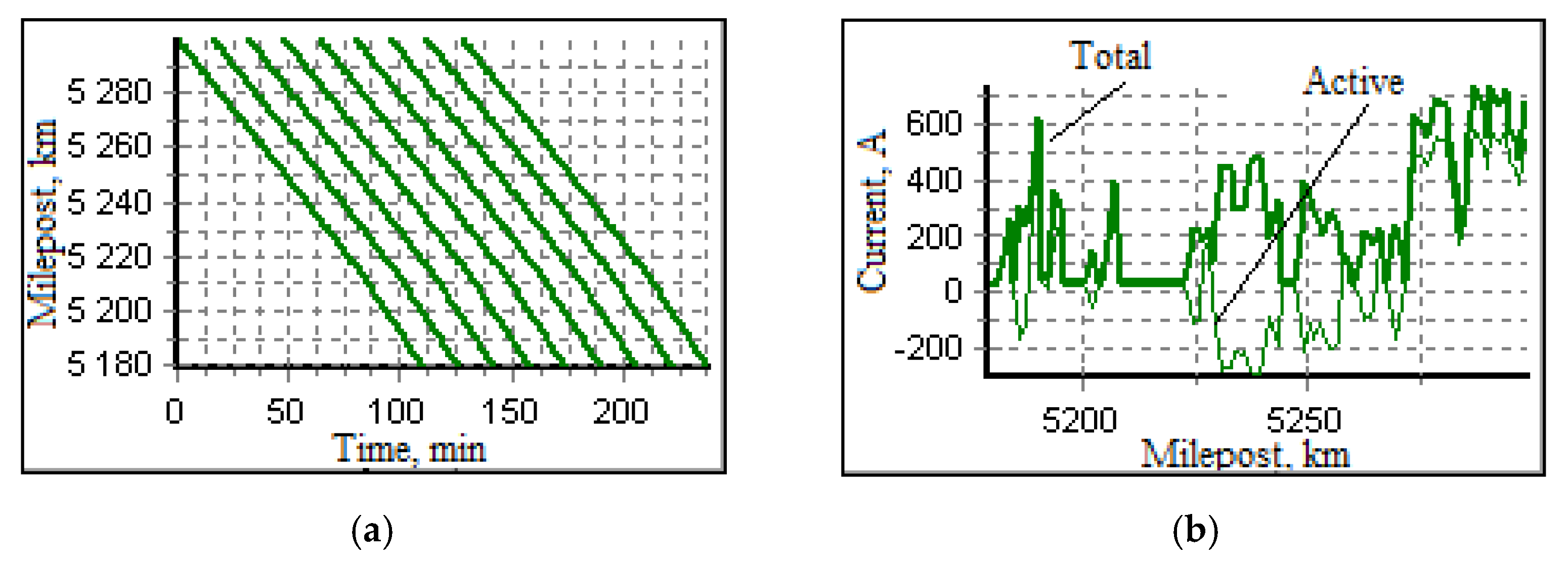
- Dynamics changes in traction loads were captured by simulating the movement of trains along real-world rail track profiles.
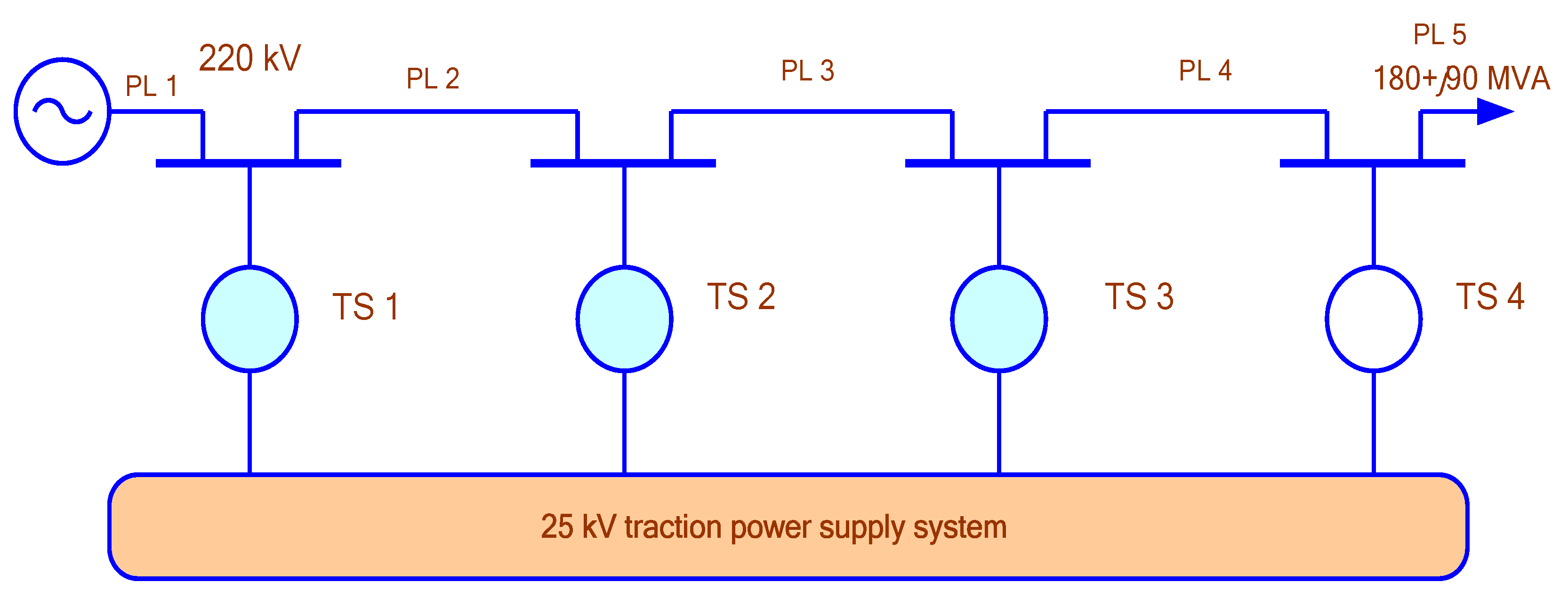
2. Object of the Study
- Possible movement of conductors within the span due to wind;
- Non-synchronous galloping;
- Galloping during ice removal;
- Possible overvoltages and constraints on corona discharge.
3. Method and Results of Modeling
- (1)
- The presence of flat conductive homogeneous earth;
- (2)
- Line wires that run parallel to each other and the ground surface;
- (3)
- Consideration of conductor current return through the ground for power transmission lines and traction networks;
- (4)
- Conductor radii that are small compared to the distances between current-carrying parts;
- (5)
- The sequence of conductor numbering is determined by the order governing the arrangement of information about them;
- (6)
- Positive directions of currents from the side external to the circuit component are assumed to be those directed towards (inside) the multi-conductor component;
- (7)
- Potentials of the nodes are counted relative to the zero-ground potential.
- Stray inductance is taken into account by connecting an inductive component in series with the coil;
- The additional magnetic flux that makes a circuit through the tank walls of the transformer and determines the zero-sequence impedance is modeled by two additional rods of a five-rod transformer;
- The relationship between field strength and induction in the transformer core is assumed to be linear;
- The two outermost rods are characterized by the complex relative magnetic permeability ; it can correspond to the magnetic permeability of the middle rods, or be taken equal to one to simulate the magnetic flux through the oil and the transformer tank. The cross-sectional areas of these rods are the same. Their lengths and magnetic permeabilities are equal to each other;
- The three middle rods of the magnetic core are characterized by a constant value of the complex magnetic permeability , determined from the nameplate values of current and no-load losses;
- Each coil has ohmic resistance and reactance , which are determined by the short-circuit parameters; here i is the winding number, which corresponds to the row of the matrix and k is the rod number minus one, or the phase number, which corresponds to the column of the matrix;
- The number of turns is determined by the effective inductance (T) in the core and the nominal voltage of the coil;
- The maximum number of transformer windings is assumed to be five.
- –
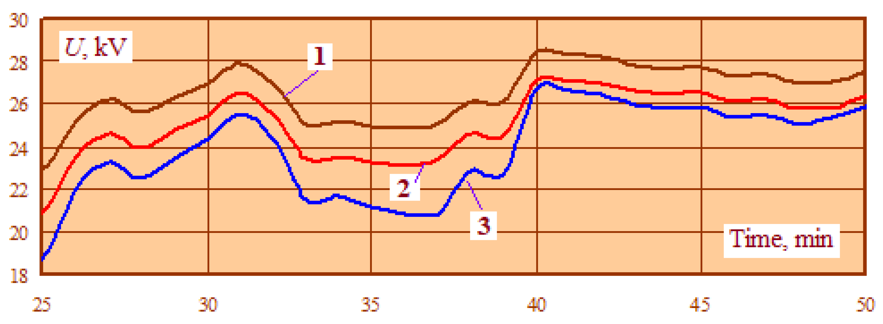
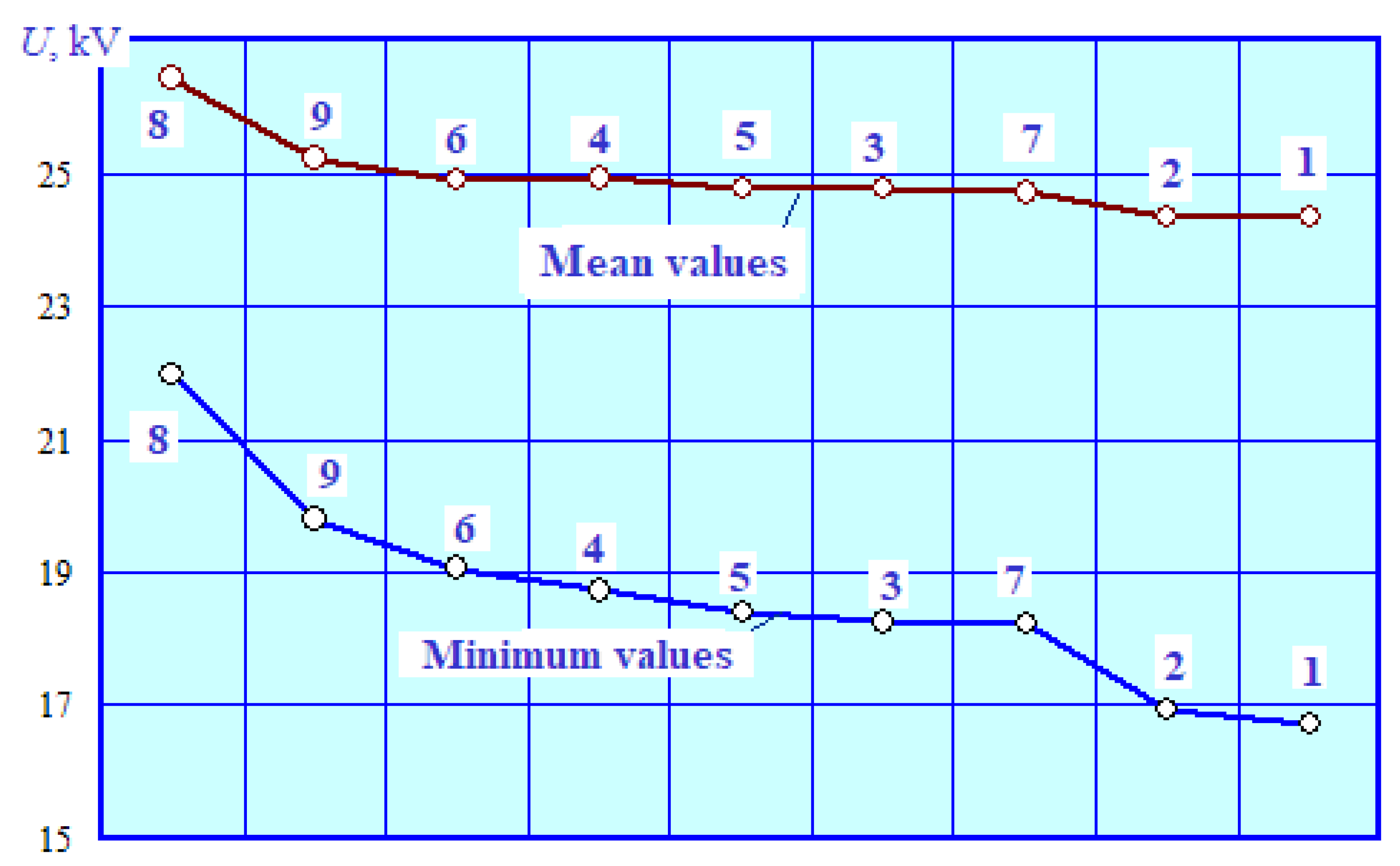
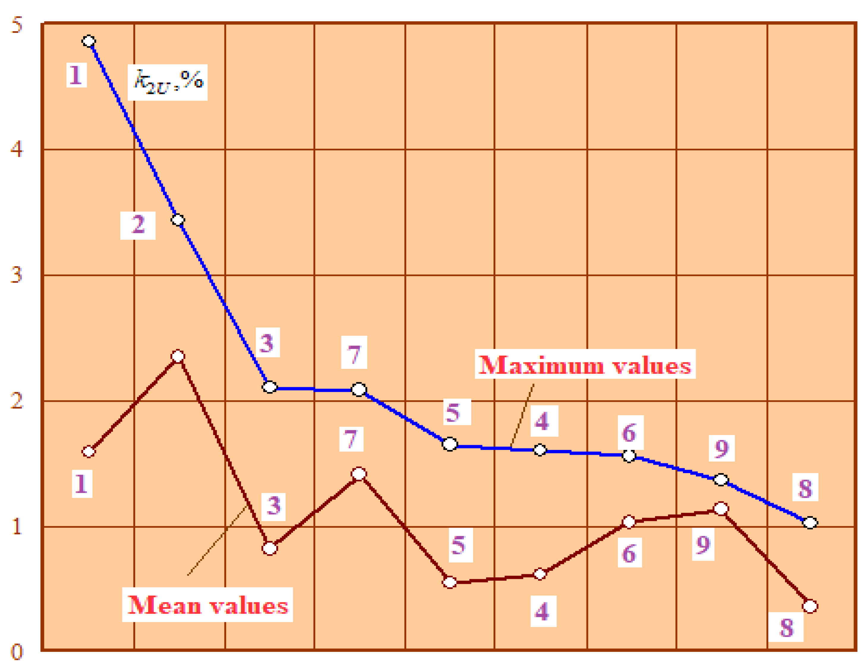
- Voltages on bow collectors of electrical rolling stock increased and stabilized (Table 1 and Figure 15). In the computational examples with a standard feeding line, voltage on the bow collector of the first train decreased below the permissible limit, and when using a three-segment COHL design it increased to 22 kV;
- –
- –
- –
- –
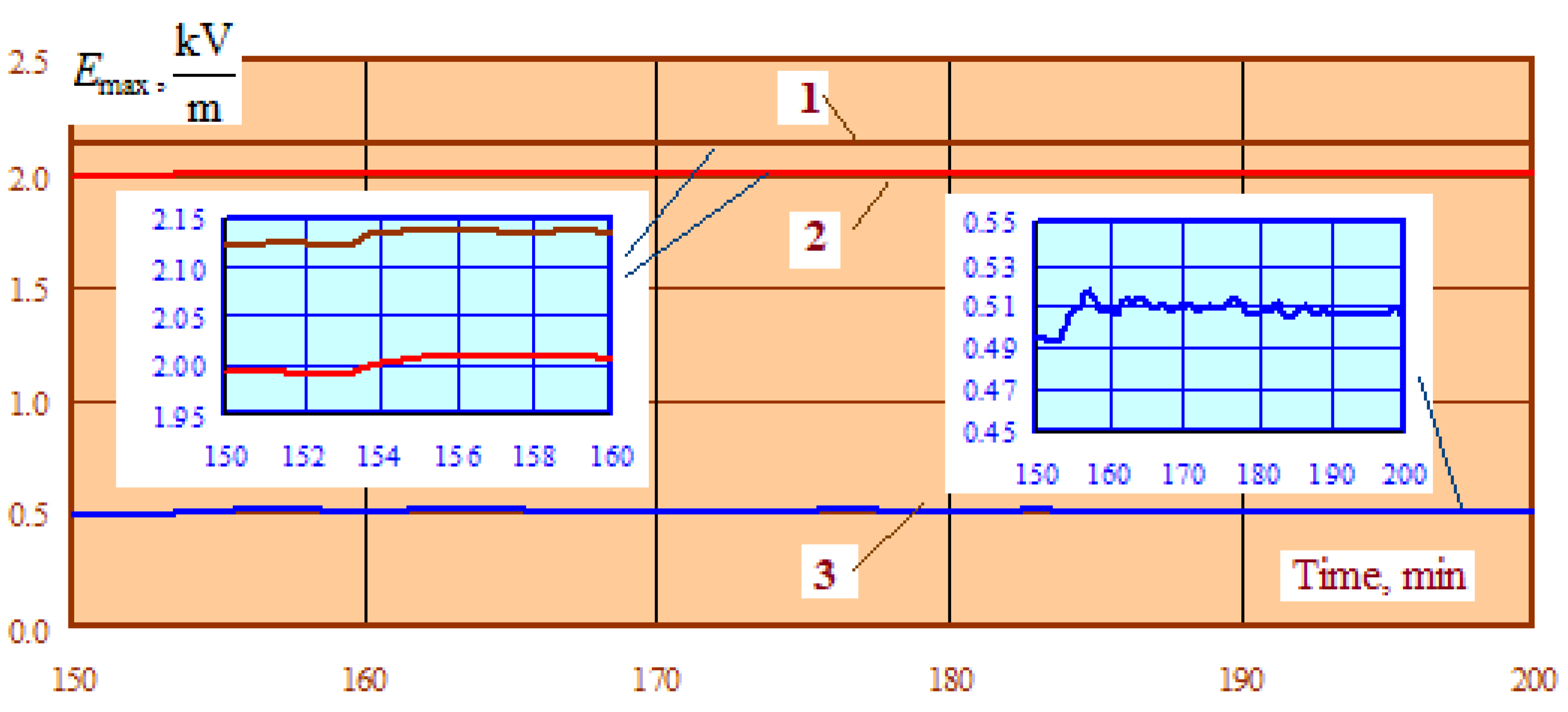
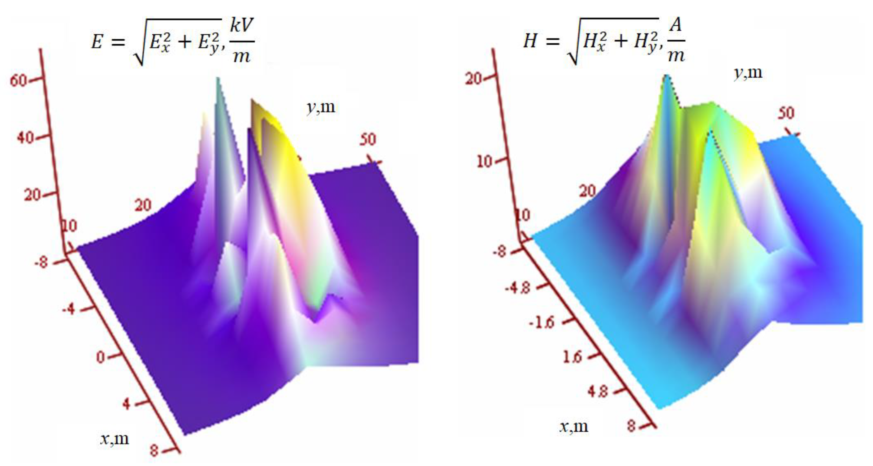
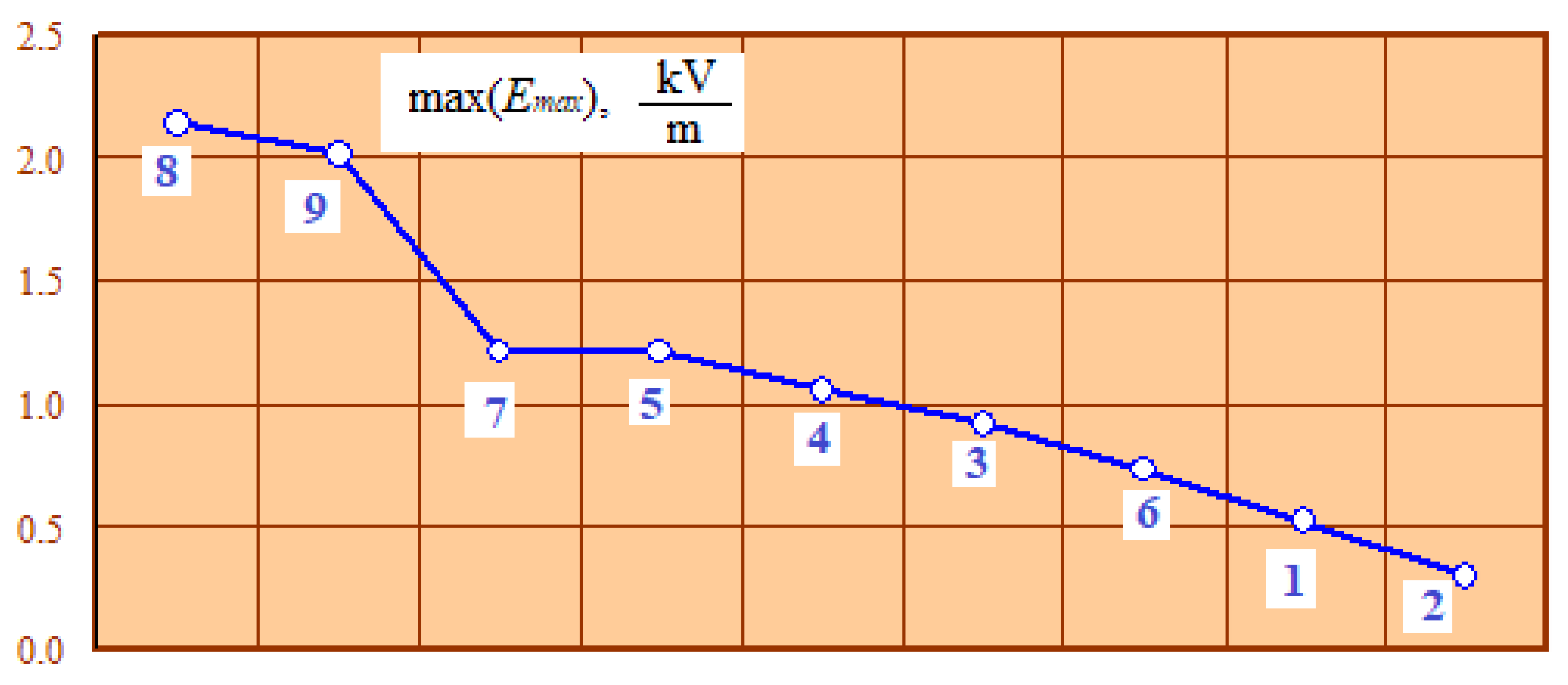
- The maximum amplitudes of the electric field (EF) of all the considered COHLs, except for the line with a vertical arrangement of wires, exceeded similar values for a standard power transmission line. The largest, fourfold, difference took place in the case of a three-segment COHL. However, the levels of EMF strengths for all the considered COHL designs did not exceed the permissible limits. Exceeding these limits only occurs when operating on a transmission line without de-energizing it (Figure 14).
- –
- –
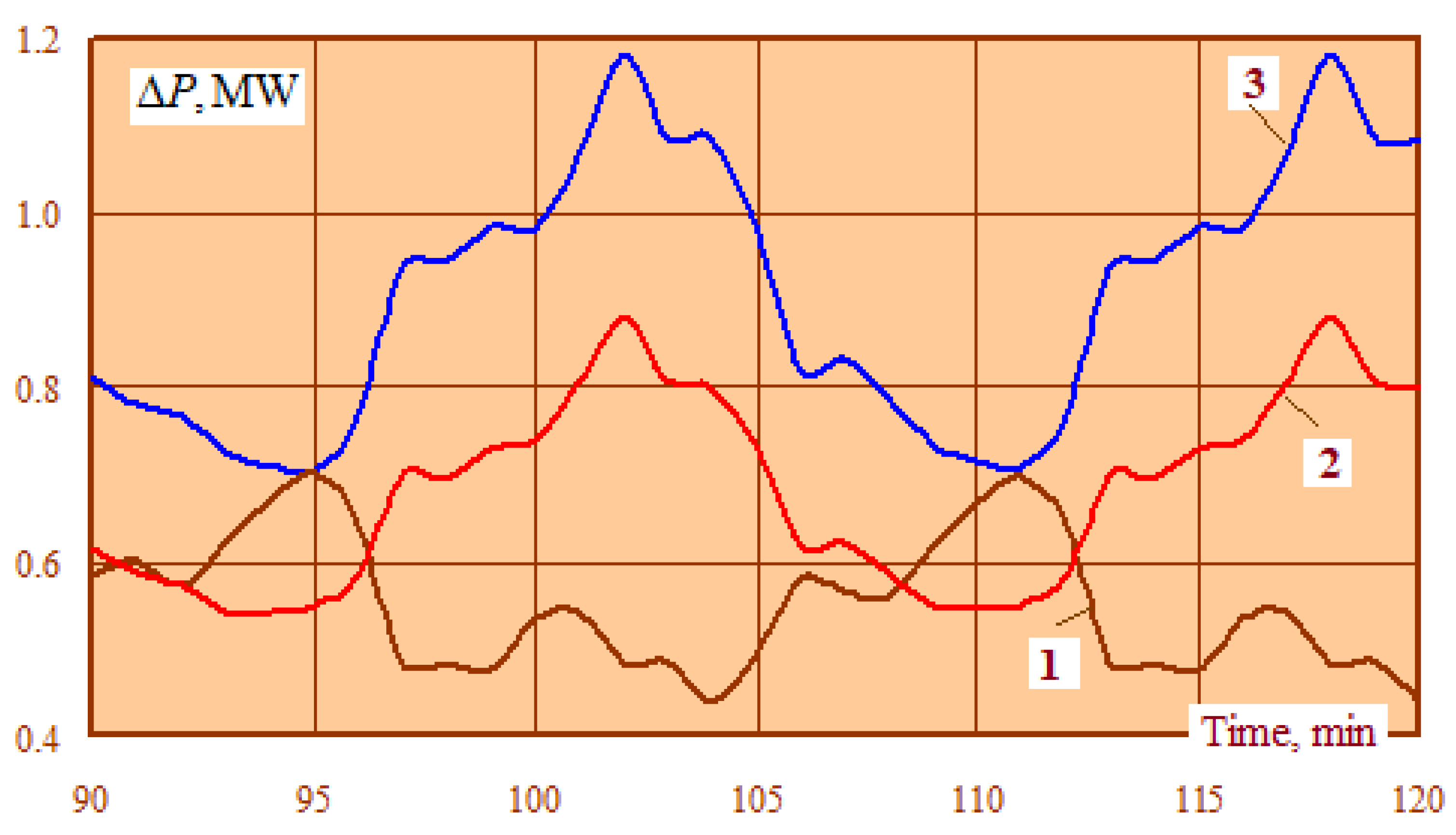
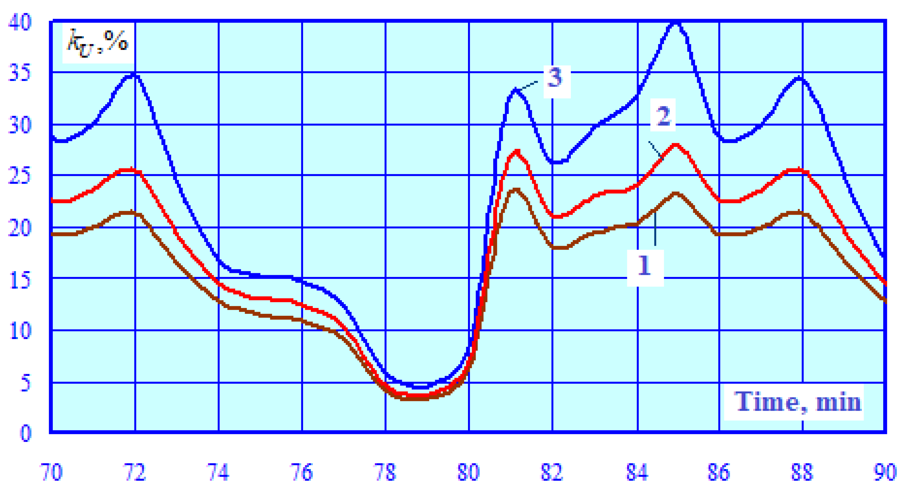
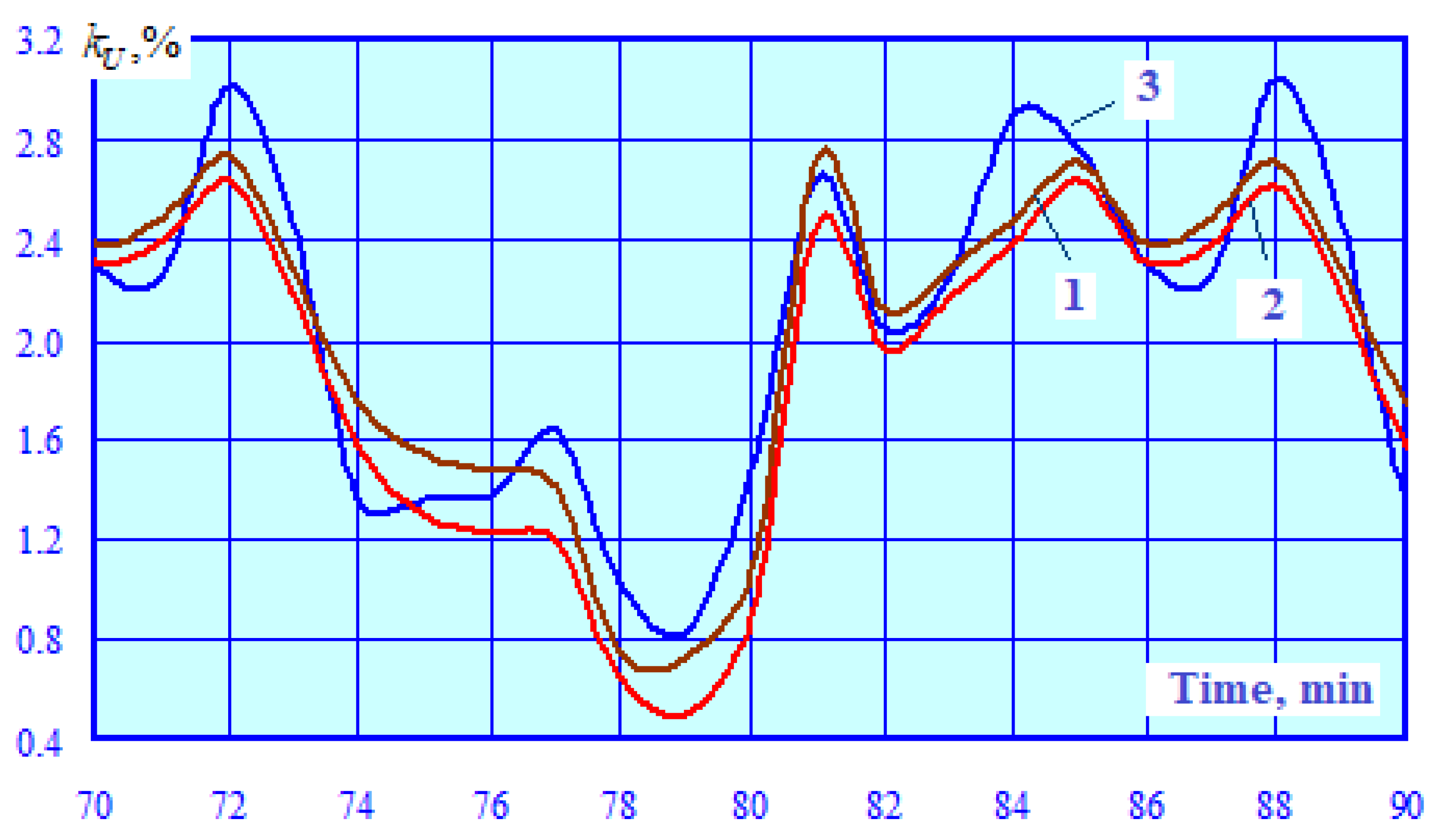
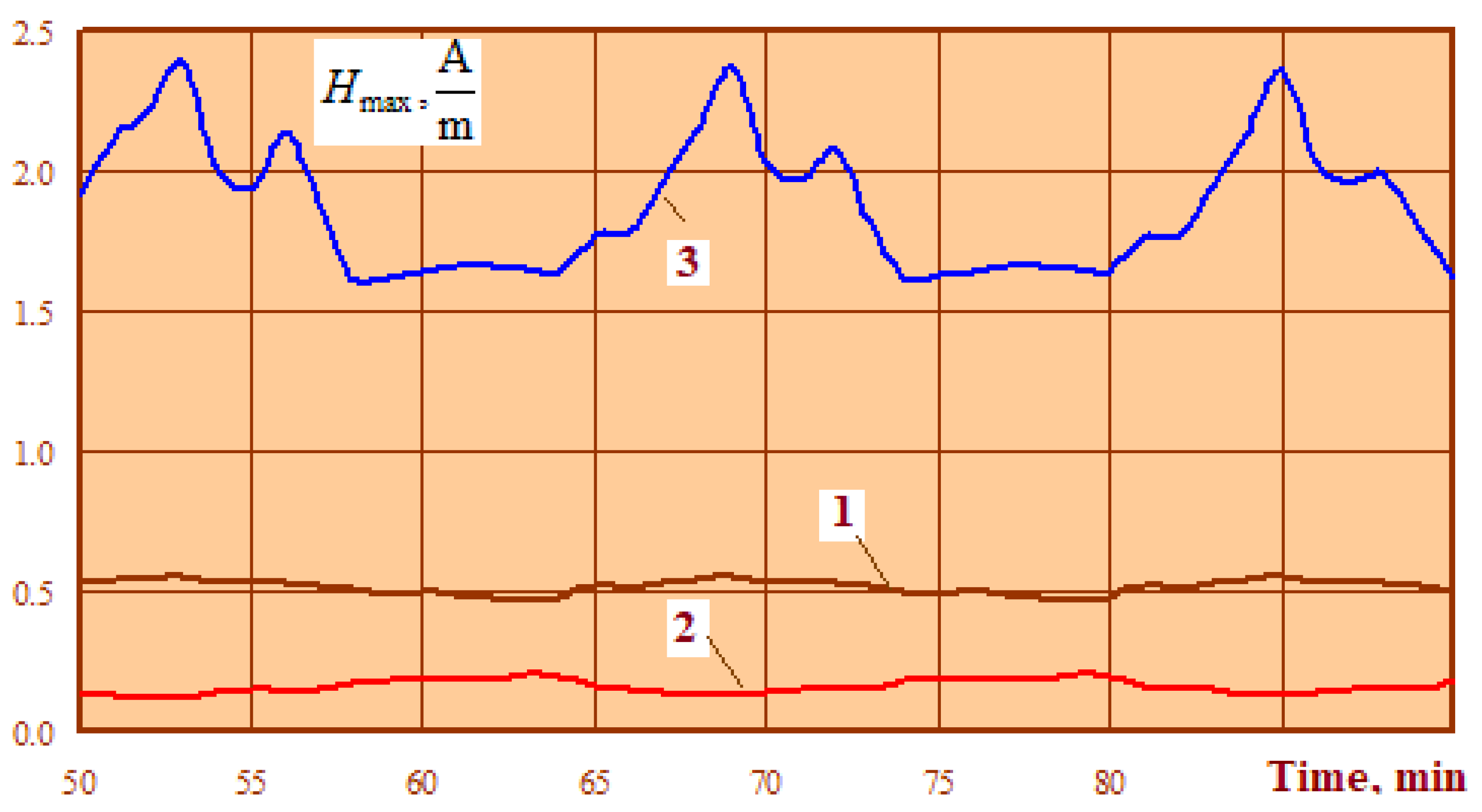
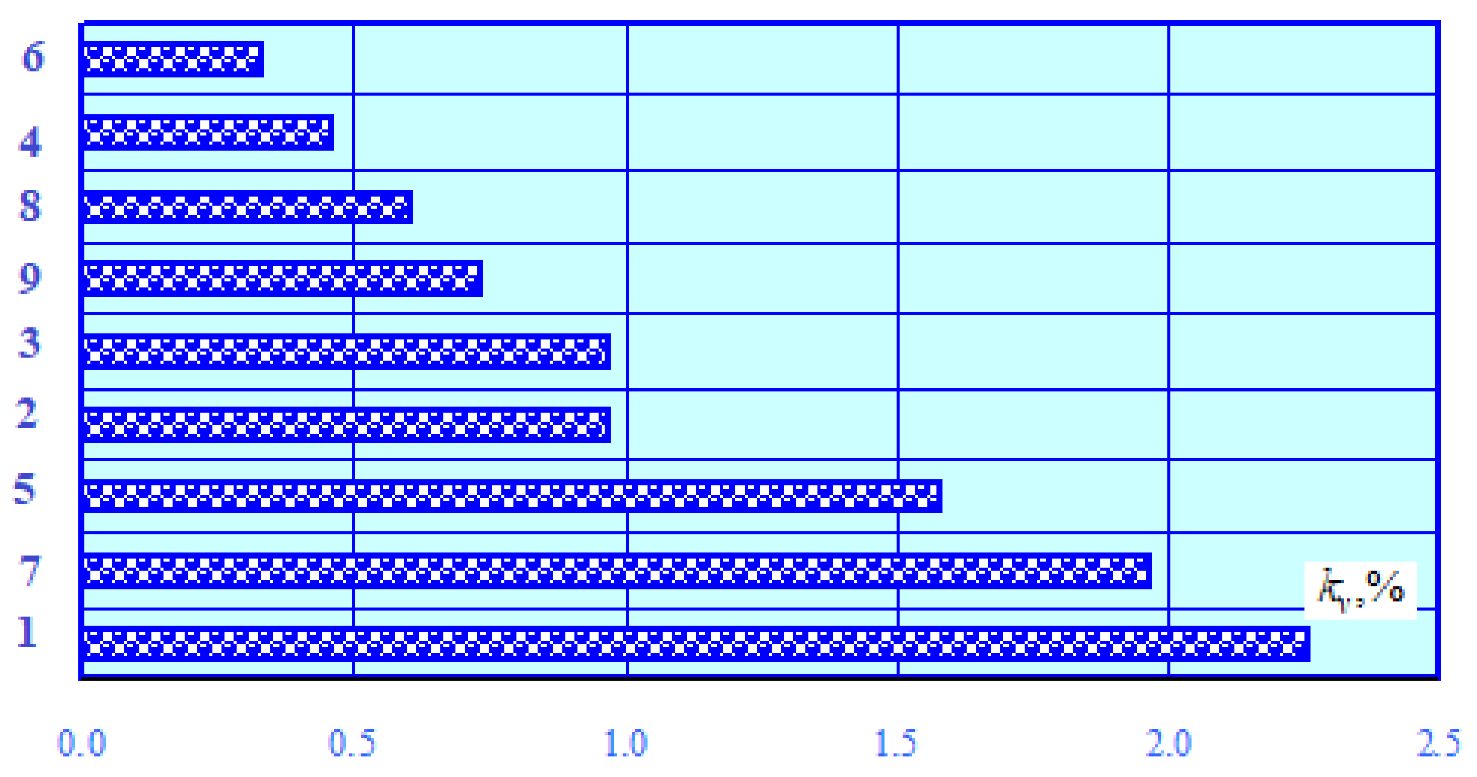
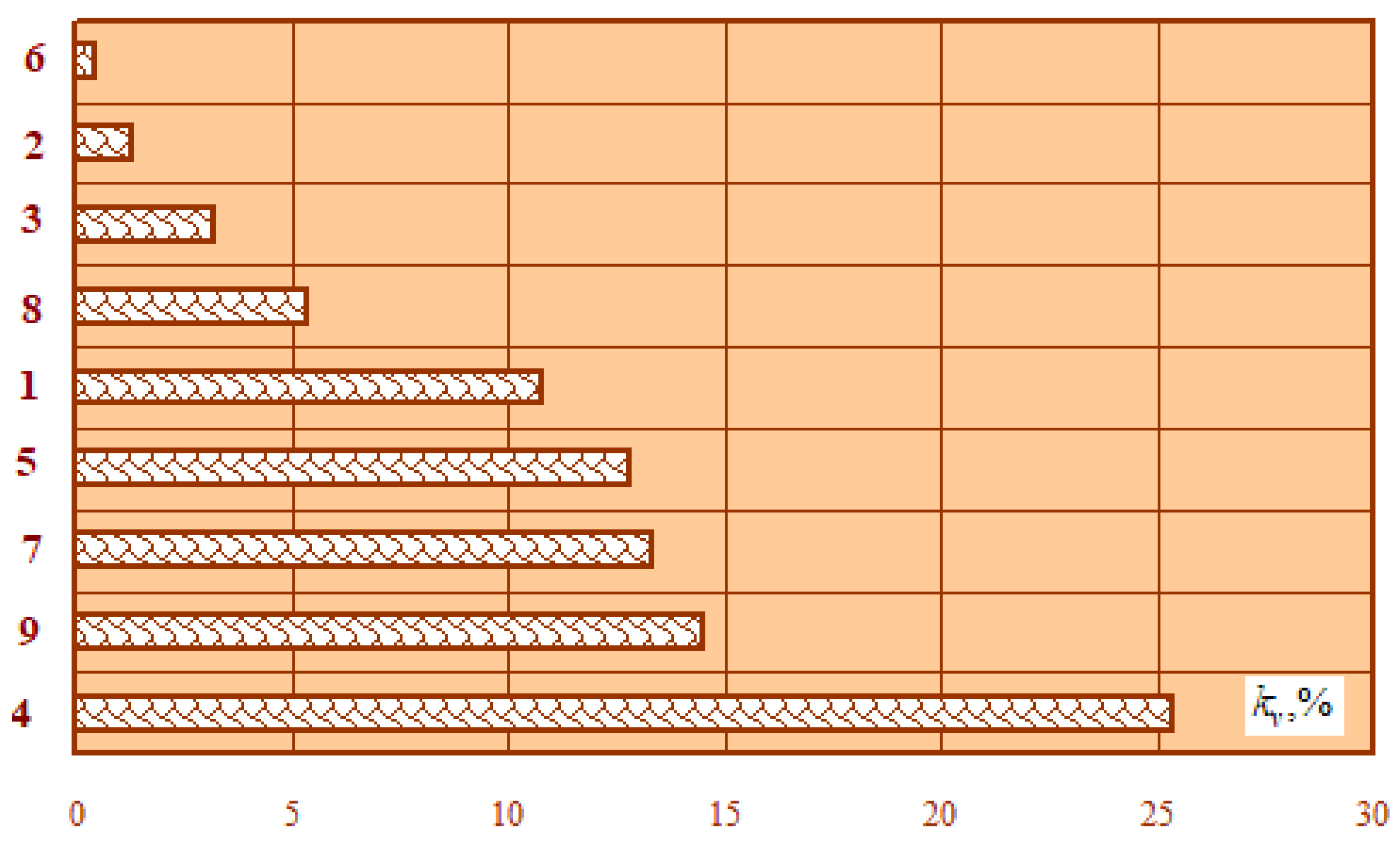
- We observed the damping effects of COHLs, which manifested themselves as the reduction of field variability. The variation coefficients of EMF strengths for all of the considered COHLs were lower than those of the standard line (Figure 23). The maximum difference was observed for the double coaxial COHL and reached seven times. MF variability that was less than in the standard line took place in the case of the following designs (Figure 24): three- and two-segment lines, coaxial double lines, and a line with a vertical arrangement of conductors.
4. Conclusions
Author Contributions
Funding
Institutional Review Board Statement
Informed Consent Statement
Data Availability Statement
Conflicts of Interest
References
- Aleksandrov, G.N. Operating Conditions of Overhead Power Transmission Lines; Energy Industry Training Center (TsPKE): Saint Petersburg, Russia, 2006; 139p. (In Russian) [Google Scholar]
- Douglass, J.; Stewart, D. Introduction to Compact Lines. In EPRI Transmission Line Reference Book—115–345kV Compact Line Design; Electric Power Research Institute: Washington, DC, USA, 2008. [Google Scholar]
- Surianu, F.-D. Determination of the induced voltages by 220 kV electric overhead power lines working in parallel and narrow routes. Measurements on the ground and mathematical model. WSEAS Trans. Power Syst. 2009, 4, 264–274. [Google Scholar]
- Zarudsky, G.K.; Samalyuk, Y.S. On considerations related to power flows of 220 V compact overhead power lines. Elektrichestvo 2013, 5, 8–13. (In Russian) [Google Scholar]
- Lavrov, Y.A.; Voitovich, R.A.; Petrova, N.F. Considerations in construction of high-voltage compact overhead power transmission lines. In Science in Russia: Promising Research and Development; Publishing house CRNS: Novosibirsk, Russia, 2017; pp. 152–159. (In Russian) [Google Scholar]
- Plotnikov, V.V.; Vasilenko, N.E.; Protasenko, I.S.; Zuev, M.M.; Zueva, T.S.; Zakutsky, V.I.; Glushkin, S.V.; Ermolov, N.S. Use of compact lines as one of the means to increase transmission capacity. Potential Mod. Sci. 2016, 4, 37–43. (In Russian) [Google Scholar]
- Postolaty, V.; Bycova, E.; Berzan, V. Compact and Controllable Electric Lines. In Proceedings of the 2019 International Conference on Electromechanical and Energy Systems (SIELMEN), Craiova, Romania, 9–11 October 2019. [Google Scholar]
- Seliverstov, G.I.; Komar, A.V.; Petrenko, V.N. Designs and parameters of compact single-circuit power transmission lines with concentric arrangement of phase conductors. ENERGETIKA 2012, 6, 41–45. (In Russian) [Google Scholar]
- Stepanov, V.M.; Karnitsky, V.Y. Compact power transmission lines. Izv. TulGU. Tekhnicheskie Nauki. 2010, 3–5, 49–51. (In Russian) [Google Scholar]
- Fedin, V.T. Innovative Engineering Solutions in Power Transmission Systems; Publishing house BNTU: Minsk, Belarus, 2012; 222p. (In Russian) [Google Scholar]
- Shakarian, Y.G.; Timashova, L.V.; Kareva, S.N. Efficiency of electric power transmission by compact controlled overhead lines. Energiya Edinoy Seti. 2014, 3, 4–15. (In Russian) [Google Scholar]
- Postolaty, V.M.; Bykova, E.V.; Suslov, V.M.; Shakaryan, Y.G.; Timashova, L.V.; Kareva, S.N. Efficiency of compact controlled high-voltage power lines. Probl. Reg. Energetics 2015, 3, 1–17. (In Russian) [Google Scholar]
- Hartono, J.; Ridwan, M.; Mafruddin, M.M.; Habibi, H.; Anugrahany, E. 500 kV quadruple circuit compact transmission line redesign study to reduce the impact of lightning strikes. In Proceedings of the 2021 3rd International Conference on High Voltage Engineering and Power Systems (ICHVEPS), Bandung, Indonesia, 5–6 October 2021. [Google Scholar]
- Jing, C.; Shanshan, Q.; Jinxiang, L.; Xiong, W.; Zongren, P. Research of Grading Ring for High Altitude 500 kV Compact Transmission Line. In Proceedings of the 2018 IEEE International Conference on High Voltage Engineering and Application (ICHVE), Athens, Greece, 10–13 September 2018. [Google Scholar]
- Buryanina, N.S.; Koroluk, Y.F.; Timofeeva, A.-M.V. 35–200 kV Compact Transmission Lines with Improved Power Transfer Capability. In Proceedings of the 2020 International Multi-Conference on Industrial Engineering and Modern Technologies (FarEastCon), Vladivostok, Russia, 6–9 October 2020. [Google Scholar]
- Shu, R.; Wei, H.; Fan, Y.; Jianbin, C.; Zhi, L. A novel equilvalent model to analyze the influence between the parallel UHVDC and EHVAC transmission lines. In 2010 Conference Proceedings IPEC; IEEE: Piscataway, NJ, USA, 2010. [Google Scholar]
- Buryanina, N.; Korolyuk, Y.; Koryakina, M.; Suslov, K.; Lesnykh, E. Compact Power Transmission Lines. In Proceedings of the 2019 International Multi-Conference on Industrial Engineering and Modern Technologies (FarEastCon), Vladivostok, Russia, 1–4 October 2019. [Google Scholar] [CrossRef]
- Dahab, A.A.; Amoura, F.K.; Abu-Elhaija, W.S. Comparison of magnetic-field distribution of noncompact and compact parallel transmission-line configurations. IEEE Trans. Power Deliv. 2005, 20, 2114–2118. [Google Scholar] [CrossRef]
- Ordon, T.J.F.; Lindsey, K.E. Considerations in the design of three phase compact transmission lines. In Proceedings of the ESMO’95—1995 IEEE 7th International Conference on Transmission and Distribution Construction, Operation and Live-Line Maintenance, Columbus, OH, USA, 29 October–3 November 1995. [Google Scholar]
- Khayam, U.; Prasetyo, R.; Hidayat, S. Electric field analysis of 150 kV compact transmission line. In Proceedings of the 2017 International Conference on High Voltage Engineering and Power Systems (ICHVEPS), Denpasar, Indonesia, 2–5 October 2017. [Google Scholar]
- Xiao, B.; Wu, T.; Liu, T.; Liu, K.; Peng, Y.; Su, Z.; Tang, P.; Lei, X. Experimental investigation on the minimum approach distance for live working on 1000kV UHV compact transmission line. In Proceedings of the In Proceedings of the 2016 IEEE International Conference on High Voltage Engineering and Application (ICHVE), Chengdu, China, 19–22 September 2016. [Google Scholar]
- Chai, X.; Liang, X.; Zeng, R. Flexible compact AC transmission system—A new mode for large-capacity and long-distance power transmission. In Proceedings of the 2006 IEEE Power Engineering Society General Meeting, Montreal, QC, Canada, 18–22 June 2006. [Google Scholar]
- Mohajeryami, S.; Doostan, M. Investigating the lightning effect on compact transmission lines by employing Monte Carlo method. In Proceedings of the 2016 IEEE/PES Transmission and Distribution Conference and Exposition (T&D), Dallas, TX, USA, 3–5 May 2016. [Google Scholar]
- Khayam, U.; Prasetyo, R.R.; Hidayat, S. Magnetic field analysis of 150 kV compact transmission line. In Proceedings of the 2017 International Conference on High Voltage Engineering and Power Systems (ICHVEPS), Denpasar, Indonesia, 2–5 October 2017. [Google Scholar]
- de Melo, M.O.B.C.; Fontana, E.; Fonseca, L.C.; Naidu, S. Lightning Protection of Compact Transmission Lines. In Proceedings of the June Conference: International conference on power systems transients, Seattle, WA, USA, 22–26 June 1997. [Google Scholar]
- Smith, D.C. Power line carrier system on a 400 kV compact delta transmission line. Trans. South Afr. Inst. Electr. Eng. 2001, 92, 16–23. [Google Scholar]
- Gong, X.; Wang, H.; Zhang, Z.; Wang, J.; Wang, J.; Yuan, Y. Tests on the first 500 kV compact transmission line in China. In Proceedings of the PowerCon 2000—2000 International Conference on Power System Technology, Perth, WA, Australia, 4–7 December 2000. [Google Scholar]
- Wei-Ming, M. The power characteristic of 500 kV large power compact overhead transmission line. In Proceedings of the TENCON’93—IEEE Region 10 International Conference on Computers, Communications and Automation, Beijing, China, 19–21 October 1993. [Google Scholar]
- Bin, Z.; Wenhui, C.; Jiayu, H. Typical models of compact transmission lines and application prospect in 500 kV AC system of China. In Proceedings of the POWERCON’98. 1998 International Conference on Power System Technology, Beijing, China, 18–21 August 1998. [Google Scholar]
- Varivodov, V.N. Compact power transmission lines. Elektro 2006, 2, 2–6. (In Russian) [Google Scholar]
- Kryukov, A.; Suslov, K.; Van Thao, L.; Hung, T.D.; Akhmetshin, A. Power Flow Modeling of Multi-Circuit Transmission Lines. Energies 2022, 15, 8249. [Google Scholar] [CrossRef]
- Bulatov, Y.; Kryukov, A.; Suslov, K. Integrated Modeling of the Modes of High Voltage Long Distance Electricity Transmission Lines. In Proceedings of the 2022 9th International Conference on Electrical and Electronics Engineering (ICEEE), Alanya, Turkey, 29–31 March 2022; pp. 45–49. [Google Scholar] [CrossRef]
- Zakaryukin, V.P.; Kryukov, A. Complex Unbalanced Load Flows of Electrical Systems; Publishing House of Irkutsk State University: Irkutsk, Russia, 2005; 273p. (In Russian) [Google Scholar]
- Zakaryukin, V.P.; Kryukov, A.V.; Le Van, T. Complex Modeling of Multi-Phase, Multi-Circuit, and Compact Power Transmission Lines; Irkutsk State Transport University (IrGUPS): Irkutsk, Russia, 2020; 296p. (In Russian) [Google Scholar]
- Carson, I.R. Wave propagation in overhead wires with ground return. Bell Syst. Tech. J. 1926, 5, 539–554. [Google Scholar] [CrossRef]


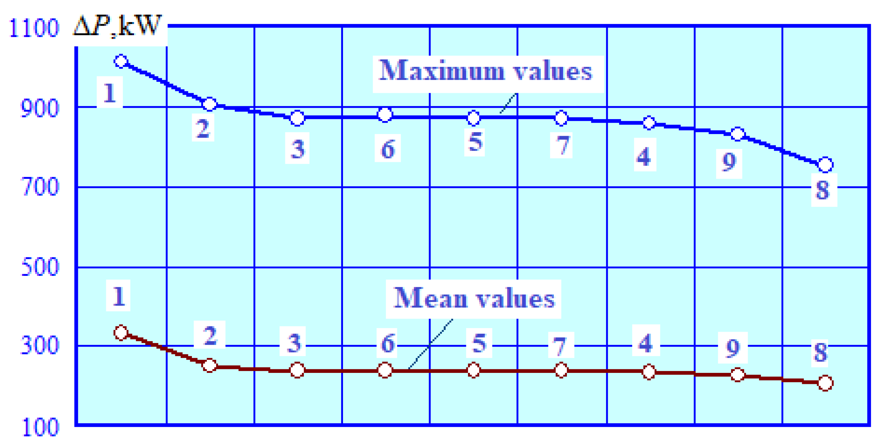
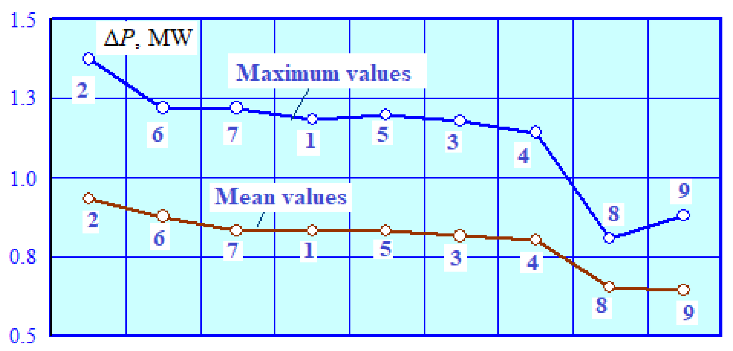
| Transmission Line Design | Umin, kV | Max(k2U), % | Max (ΔPTN), kW | Max (ΔPTL), MW |
|---|---|---|---|---|
| Standard power transmission line with AS-600 conductors | 16.73 | 4.86 | 1015 | 1.18 |
| COHL with a vertical arrangement of conductors | 16.93 | 3.43 | 906 | 1.37 |
| Coaxial two-segment COHL | 18.24 | 2.1 | 872 | 1.18 |
| Coaxial four-segment COHL | 18.72 | 1.6 | 857 | 1.14 |
| COHL with a delta arrangement of conductors | 18.41 | 1.64 | 872 | 1.2 |
| Double coaxial COHL | 19.05 | 1.55 | 880 | 1.22 |
| COHL with a parabolic arrangement of conductors | 18.21 | 2.08 | 871 | 1.22 |
| COHL with a three-segment arrangement of conductors | 21.98 | 1.02 | 753 | 0.81 |
| COHL with a concentric arrangement of conductors | 19.76 | 1.37 | 832 | 0.88 |
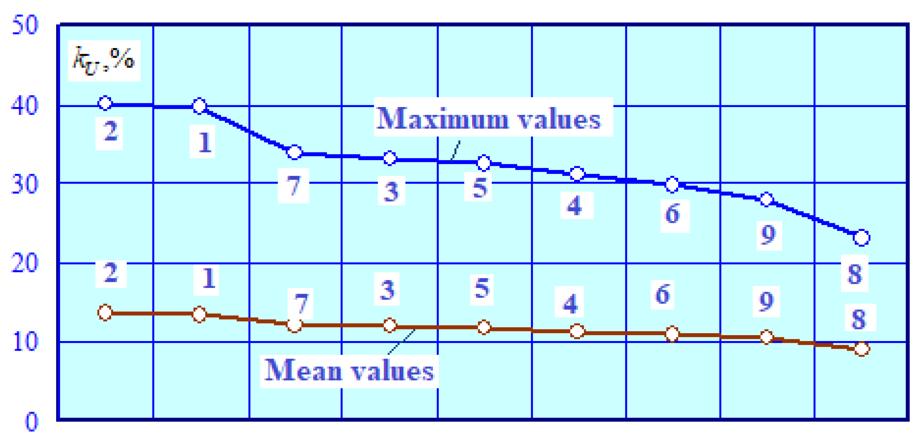
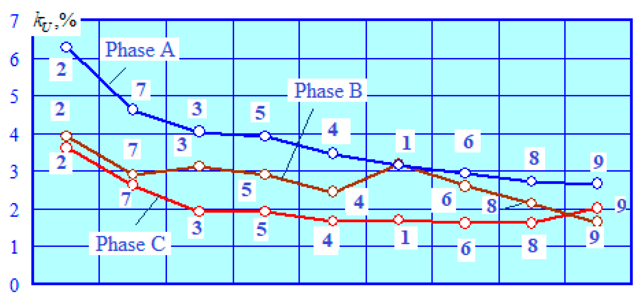
| Transmission Line Design | kU220, % | kU27.5, % | Emax, kV/m | Hmax, A/m |
|---|---|---|---|---|
| Standard power transmission line with AS-600 conductors | 3.17 | 39.74 | 0.52 | 2.39 |
| COHL with a vertical arrangement of conductors | 6.31 | 40.14 | 0.33 | 0.94 |
| Coaxial two-segment COHL | 4.05 | 33.19 | 0.92 | 0.66 |
| Coaxial four-segment COHL | 3.48 | 31.13 | 1.05 | 0.25 |
| COHL with a delta arrangement of conductors | 3.92 | 23.19 | 1.21 | 0.8 |
| Double coaxial COHL | 2.96 | 29.8 | 0.73 | 1.2 |
| COHL with a parabolic arrangement of conductors | 4.64 | 33.8 | 1.21 | 0.78 |
| COHL with a three-segment arrangement of conductors | 2.75 | 23.19 | 2.14 | 0.55 |
| COHL with a concentric arrangement of conductors | 2.68 | 27.87 | 2.01 | 0.22 |
Disclaimer/Publisher’s Note: The statements, opinions and data contained in all publications are solely those of the individual author(s) and contributor(s) and not of MDPI and/or the editor(s). MDPI and/or the editor(s) disclaim responsibility for any injury to people or property resulting from any ideas, methods, instructions or products referred to in the content. |
© 2023 by the authors. Licensee MDPI, Basel, Switzerland. This article is an open access article distributed under the terms and conditions of the Creative Commons Attribution (CC BY) license (https://creativecommons.org/licenses/by/4.0/).
Share and Cite
Suslov, K.; Kryukov, A.; Voronina, E.; Fesak, I. Modeling Power Flows and Electromagnetic Fields Induced by Compact Overhead Lines Feeding Traction Substations of Mainline Railroads. Appl. Sci. 2023, 13, 4249. https://doi.org/10.3390/app13074249
Suslov K, Kryukov A, Voronina E, Fesak I. Modeling Power Flows and Electromagnetic Fields Induced by Compact Overhead Lines Feeding Traction Substations of Mainline Railroads. Applied Sciences. 2023; 13(7):4249. https://doi.org/10.3390/app13074249
Chicago/Turabian StyleSuslov, Konstantin, Andrey Kryukov, Ekaterina Voronina, and Ilia Fesak. 2023. "Modeling Power Flows and Electromagnetic Fields Induced by Compact Overhead Lines Feeding Traction Substations of Mainline Railroads" Applied Sciences 13, no. 7: 4249. https://doi.org/10.3390/app13074249