

Simulation of Cross-Correlated Random Fields for Transversely Anisotropic Soil Slope by Copulas
Abstract
:1. Introduction
2. Random Field Theory
2.1. Overview
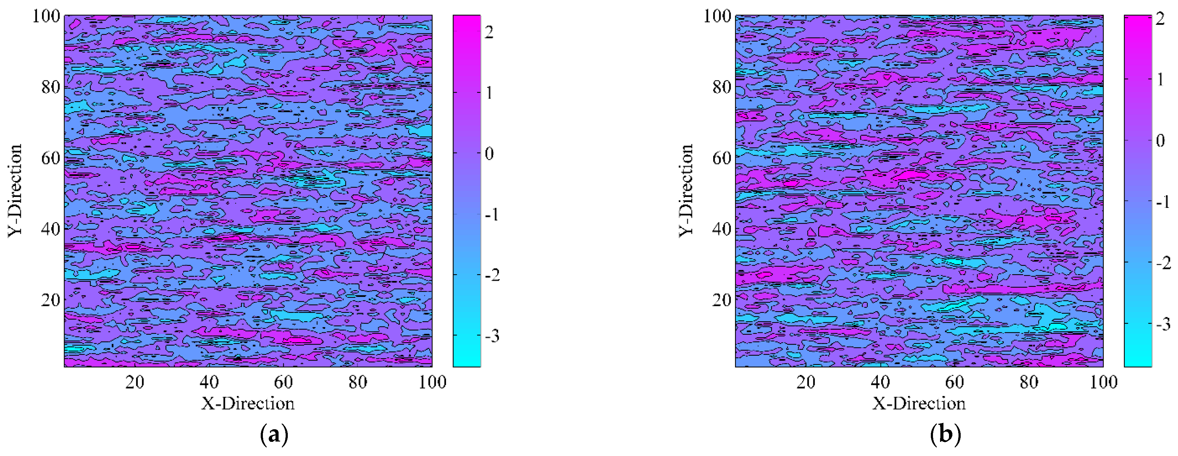
2.2. Transversely Anisotropic Random Field
2.3. Discretization of Transversely Anisotropic Random Field
3. Copula Theory
4. Simulation of CCRF from Copula Aspect
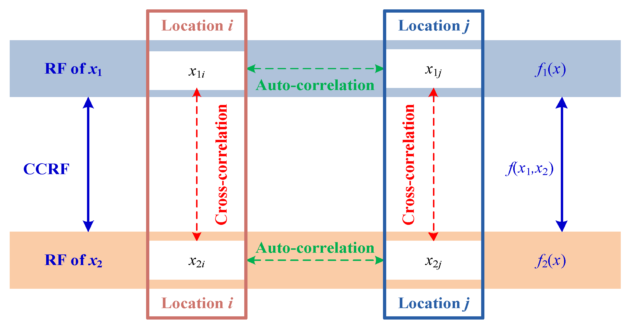
4.1. Cross-Correlation of Soil Parameters
4.2. Transformation of CCRF by Copulas
| Algorithm 1 Simulation algorithm of copula-based standard uniform CCRF |
| (1) Define the correlation structure between multivariate correlation standard uniform random fields as Ci = C (H1CAU, H2CAU, ⋯, HiCAU), where i = 2, 3, ⋯, n; (2) Extract H1IAU from the standard uniform distribution U(0, 1), let H1CAU = H1IAU; (3) Extract H2CAU from C2 (H2CAU|H1CAU); (4) Similarly, extract HnCAU from Cn (HnCAU|H1CAU, H2CAU, ⋯, Hn−1CAU). |
4.3. Gaussian Copula-Based CCRF
| Algorithm 2 Simulation algorithm of Gaussian copula-based CCRF |
| (1) Define the independent standard normal random fields of x and y as HIAG = [ HxIAG, HyIAG ]T. (2) Perform Cholesky decomposition on the correlation coefficient matrix θ composed of Gaussian copula parameter θ to obtain the lower triangular matrix L0. (3) Let HCAG = L0HIAG, then the cross-correlation standard normal random fields HCAG = [HxCAG, HyCAG ]T can be obtained. (4) Let HCAU = Φ(HCAG), where Φ(·) is the CDF of the standard normal distribution, and the cross-correlation standard uniform random fields of x and y can be obtained HCAU = [HxCAU, HyCAU ]T. (5) Define Fx−1(·) and Fy−1(·) as the inverse functions of the CDF of x and y, respectively. Perform isoprobabilistic transformation on HCAU to obtain the cross-correlation non-normal random fields of x and y HCAN = [HxCAN, HyCAN ]T = [Fx−1(HxCAU), Fy−1(HyCAU)]T. |
4.4. Plackett Copula-Based CCRF
| Algorithm 3 Simulation algorithm of Plackett copula-based CCRF |
| (1) Define the independent standard normal random fields x and y HIAG = [HxIAG, HyIAG ]T. (2) Let HIAU = Φ(HIAG), then the independent standard uniform random fields of x and y HIAU = [HxIAU, HyIAU]T can be obtained. (3) Define a = HyIAU (1−HyIAU), b =θ +a(θ−1)2, c = 2a (HxIAUθ2 + 1-HxIAU) + θ (1–2a0), d = θ1/2[ θ + 4aHxIAU(1−HxIAU)(1−θ)2 ]1/2. (4) Let HxCAU = HxIAU, HyCAU = [c-(1–2HyIAU)d ]/2b, and obtain the cross-correlation standard uniform random fields x and y HCAU = [ HxCAU, HyCAU]T. (5) Use Fx−1(·) and Fy−1(·) to perform isoprobabilistic transformation on HCAU = [HxCAU, HyCAU]. Then the cross-correlation non-normal random fields of x and y HCAN = [HxCAN, HyCAN ]T = [Fx−1(HxCAU), Fy−1(HyCAU)]T can be obtained. |
4.5. Frank Copula-Based CCRF
| Algorithm 4 Simulation algorithm of Frank copula-based CCRF |
| (1) Define the independent standard normal random fields of x and y HIAG = [HxIAG, HyIAG ]T. (2) Let HIAU = Φ(HIAG), then the independent standard uniform random fields of x and y HIAU = [HxIAU, HyIAU]T can be obtained. (3) Let HxCAU = HxIAU, HyCAU be inversely calculated according to the Frank copula, as shown below: (4) Solve the above equation in (3) to get the cross-correlation standard uniform random fields HCAU = [HxCAU, HyCAU]T of x and y. (5) Use Fx−1(·) and Fy−1(·) to perform isoprobabilistic transformation on HCAU = [HxCAU, HyCAU]. Then the cross-correlation non-normal random fields of x and y HCAN = [HxCAN, HyCAN ]T = [Fx−1(HxCAU), Fy−1(HyCAU)]T can be obtained. |
4.6. No. 16 Copula-Based CCRF
| Algorithm 5 Simulation algorithm of No. 16 copula-based CCRF |
| (1) Define the independent standard normal random fields of x and y as HIAG = [ HxIAG, HyIAG ]T. (2) Let HIAU = Φ(HIAG), then the independent standard uniform random fields of x and y HIAU = [HxIAU, HyIAU]T can be obtained. (3) Let HxCAU = HxIAU, HyCAU be calculated according to the following equation: (4) Solve equations in (3) to get the cross-correlation standard uniform random fields HCAU = [HxCAU, HyCAU]T of x and y. (5) Use Fx−1(·) and Fy−1(·) to perform isoprobabilistic transformation on HCAU = [HxCAU, HyCAU]. Then the cross-correlation non-normal random fields of x and y HCAN = [HxCAN, HyCAN ]T = [Fx−1(HxCAU), Fy−1(HyCAU)]T can be obtained. |
5. Simulation Process of Transversely Anisotropic CCRF
6. Numerical Illustrations
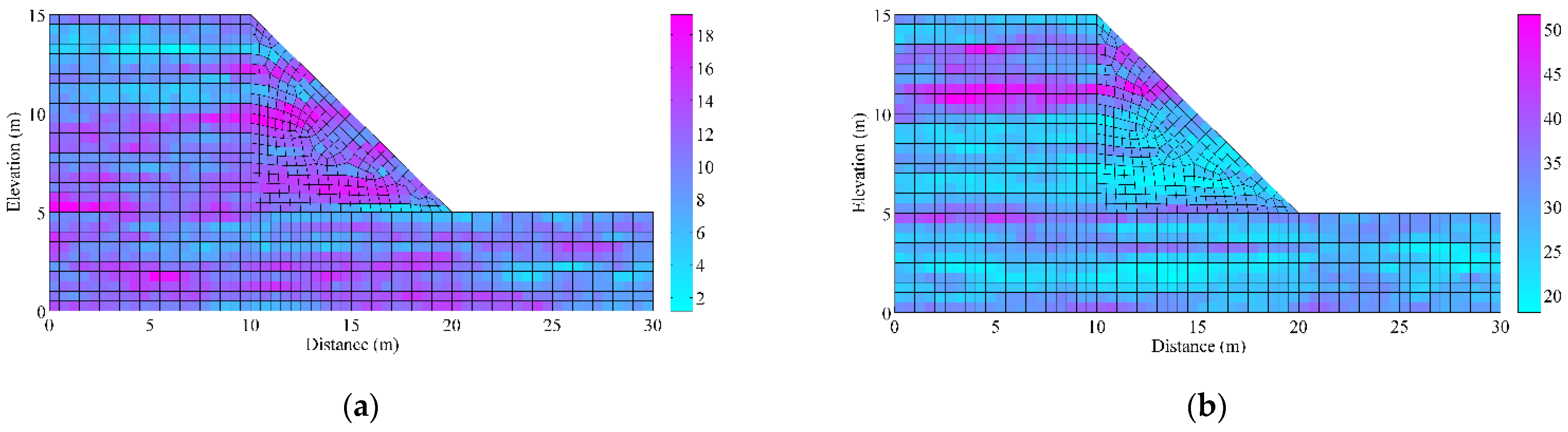
6.1. Example 1: Assumed c-ϕ Soil Slope
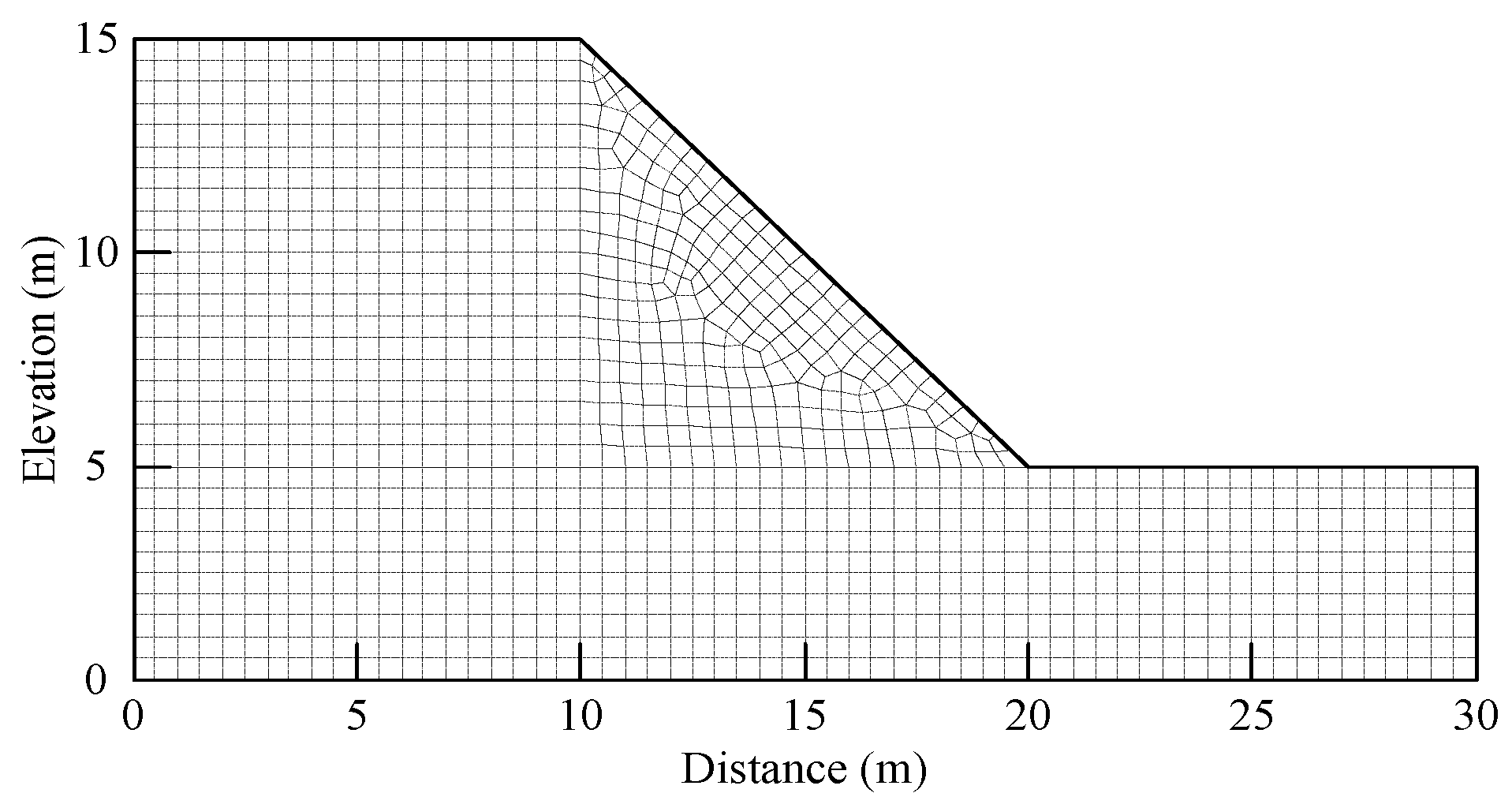
6.1.1. Profiles of c-ϕ Soil Slope
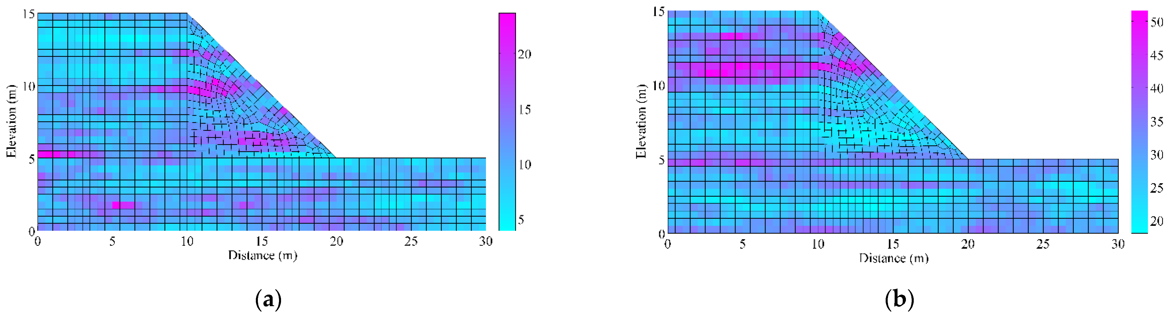
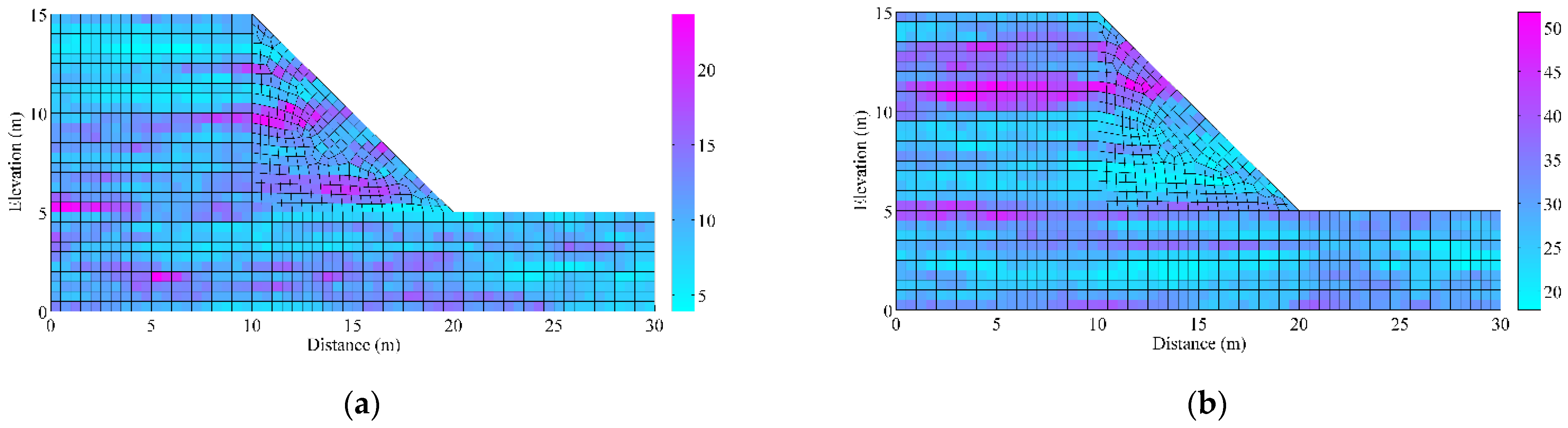
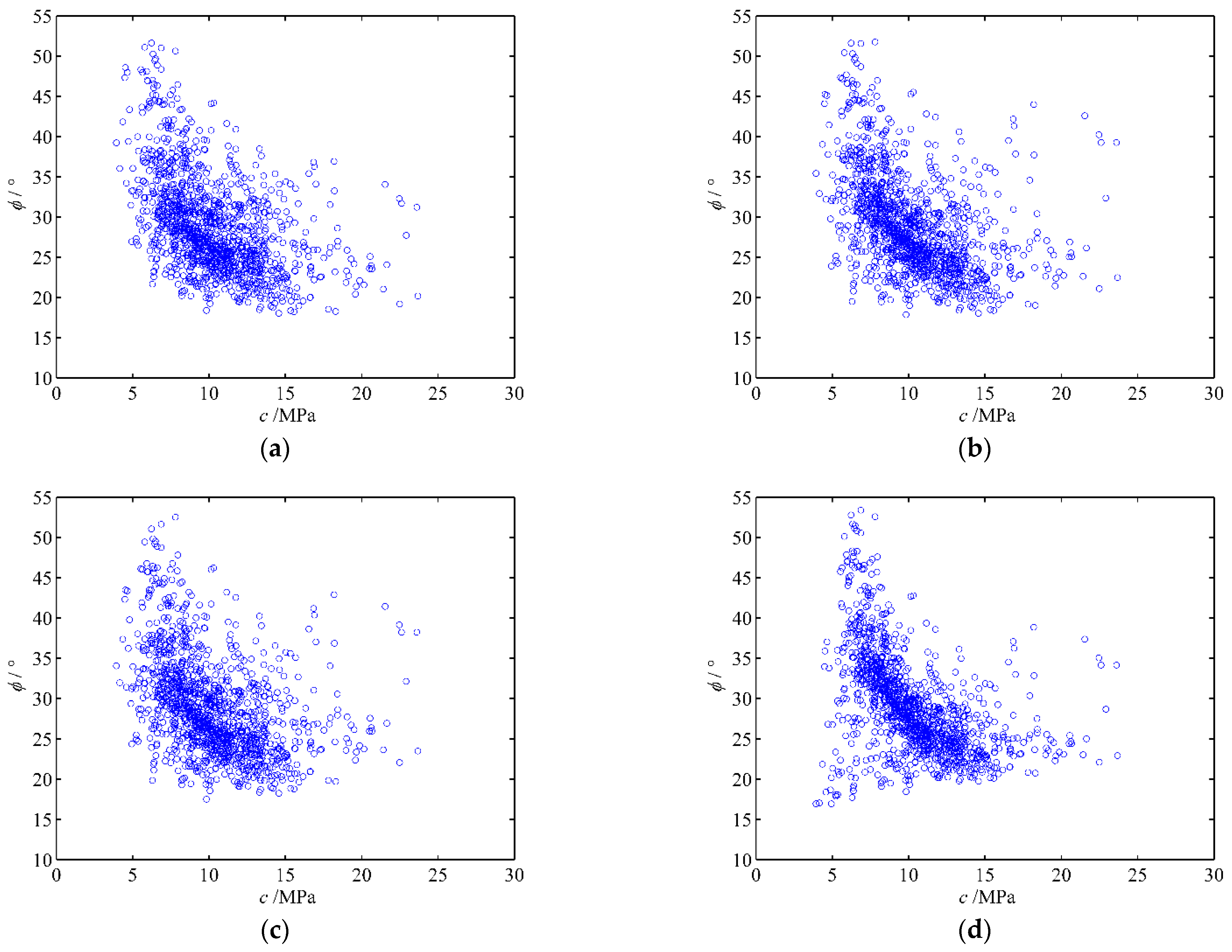
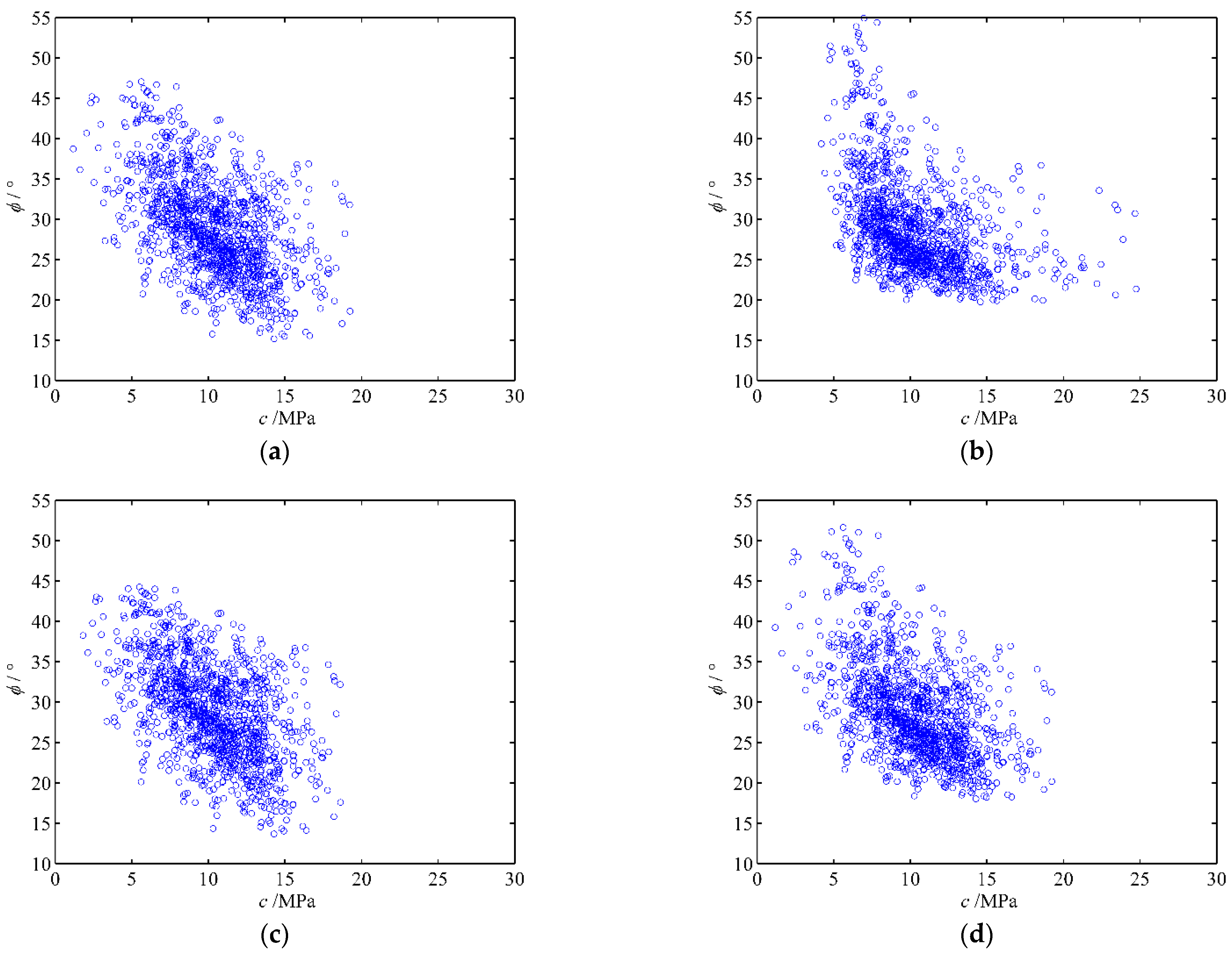
6.1.2. Simulation of CCRF
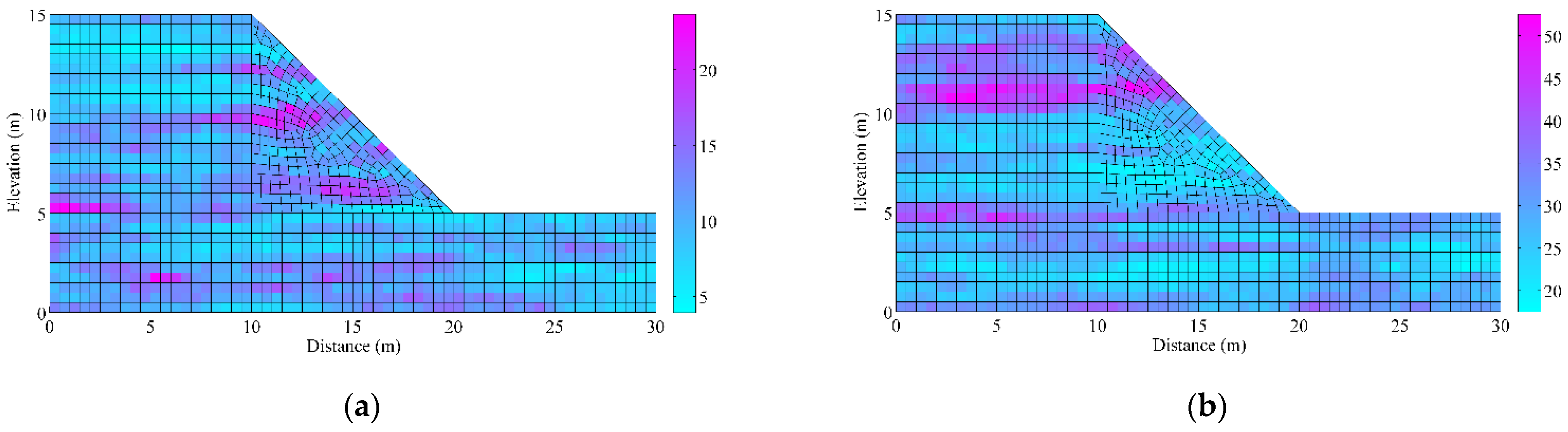
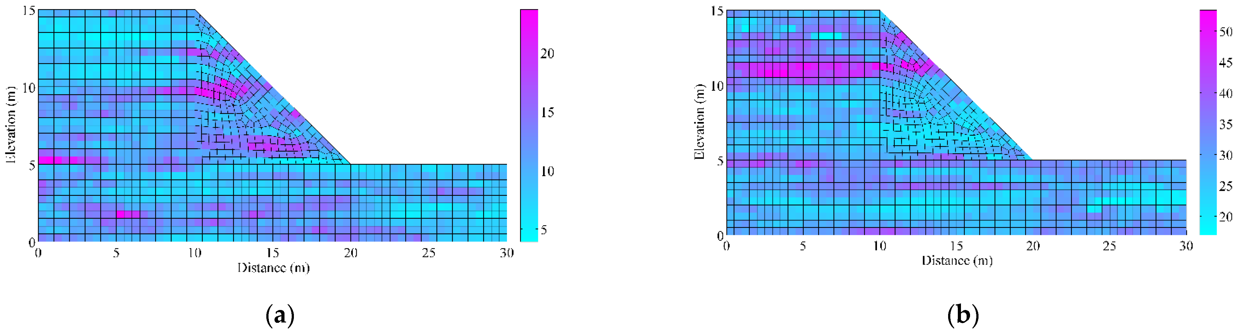
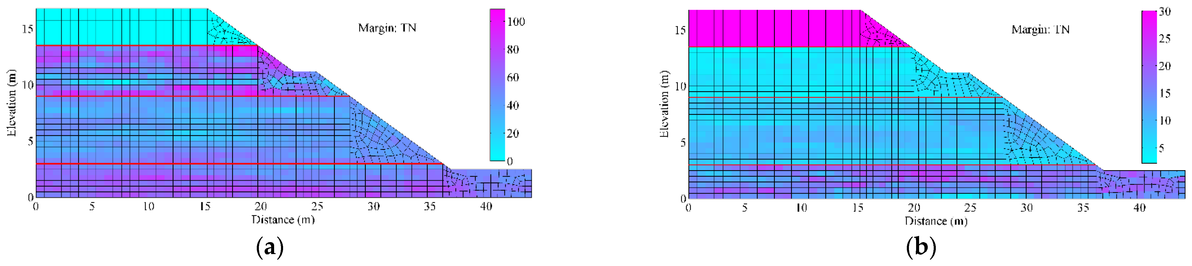
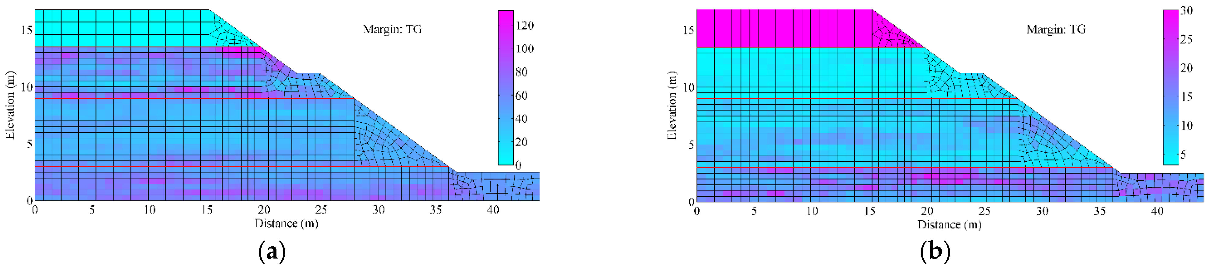
6.1.3. Effect of Marginal Distribution on CCRF
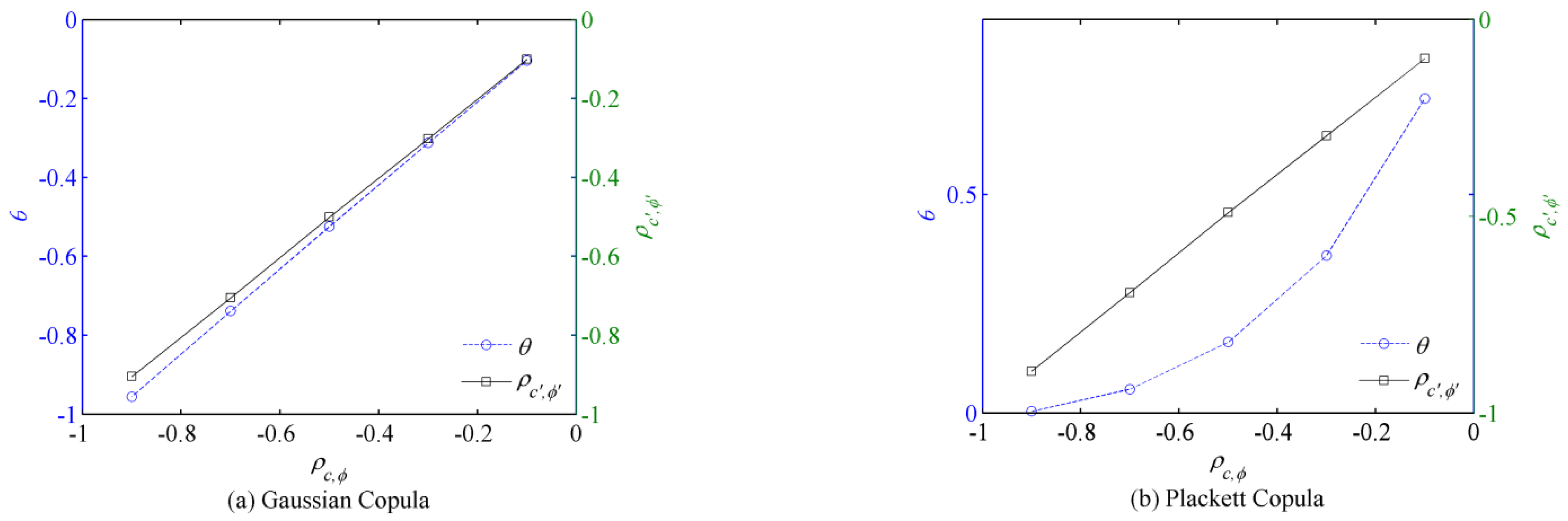
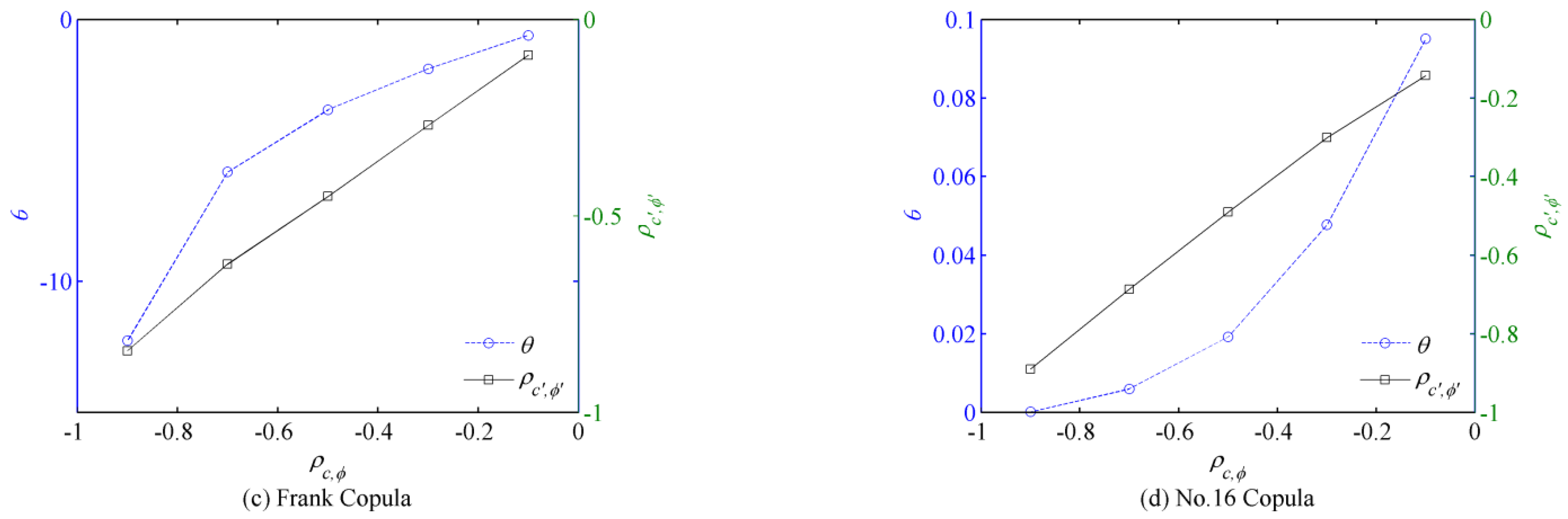
6.1.4. Effect of Correlation Coefficient on CCRF
6.2. Example 2: Chicago Congress Street Cut Slope
6.2.1. The Profile of Chicago Congress Street Cut Slope
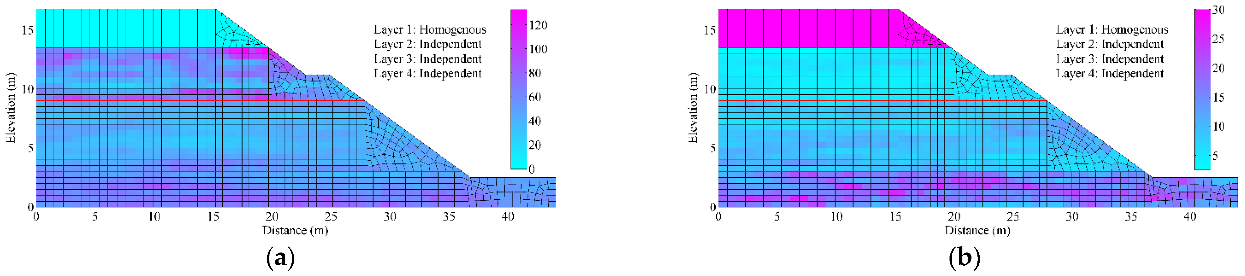
6.2.2. Simulation of Multi-Layer CCRF
6.3. Example 3: Papillion River Basin Slope
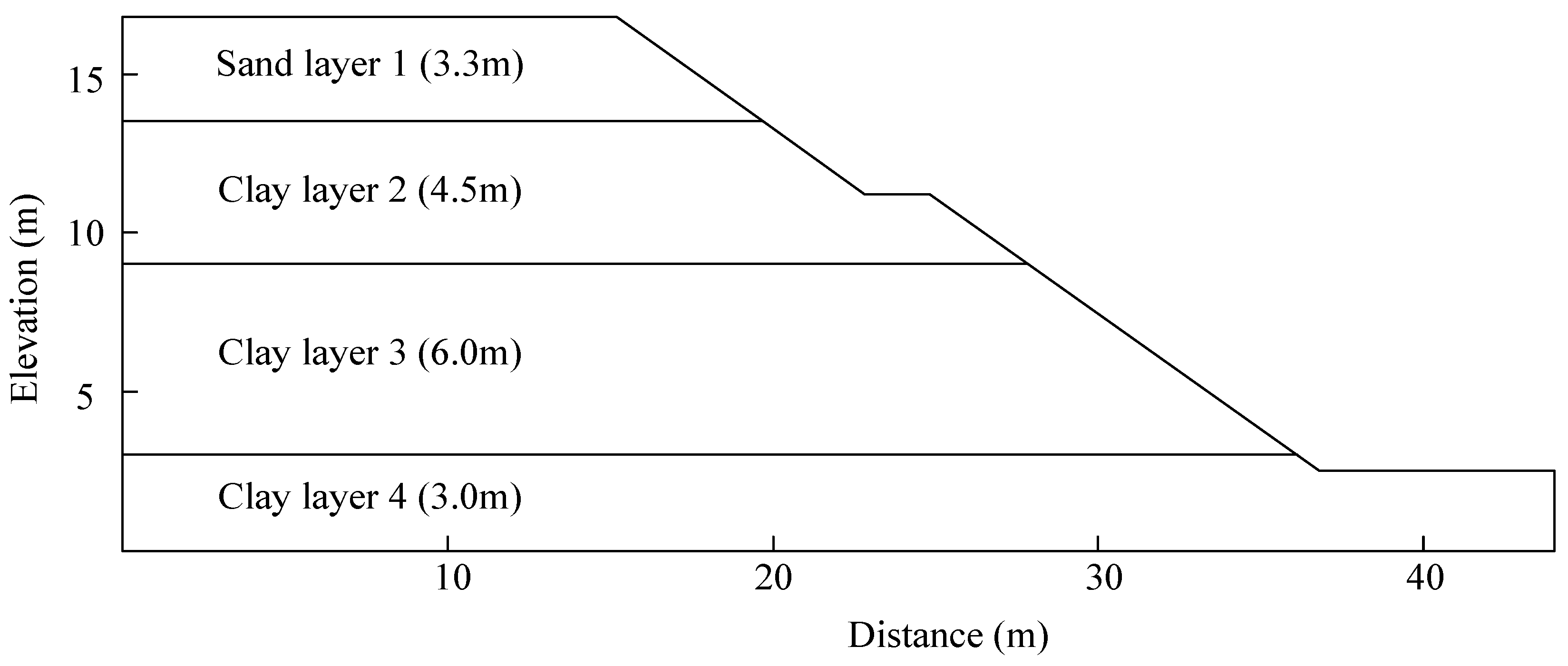
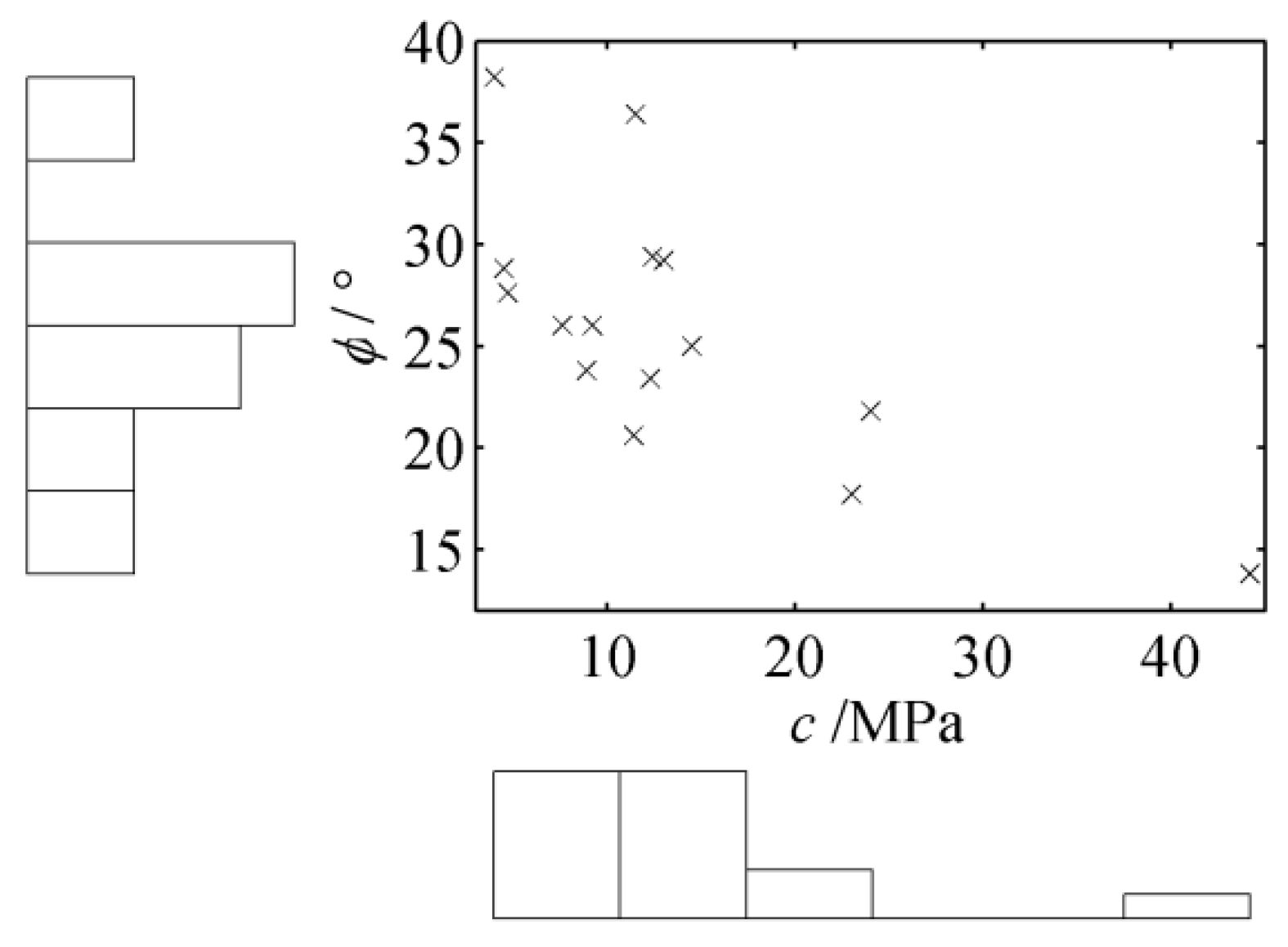
6.3.1. Soil Profile
6.3.2. Probability Distribution Estimation of Soil Parameters
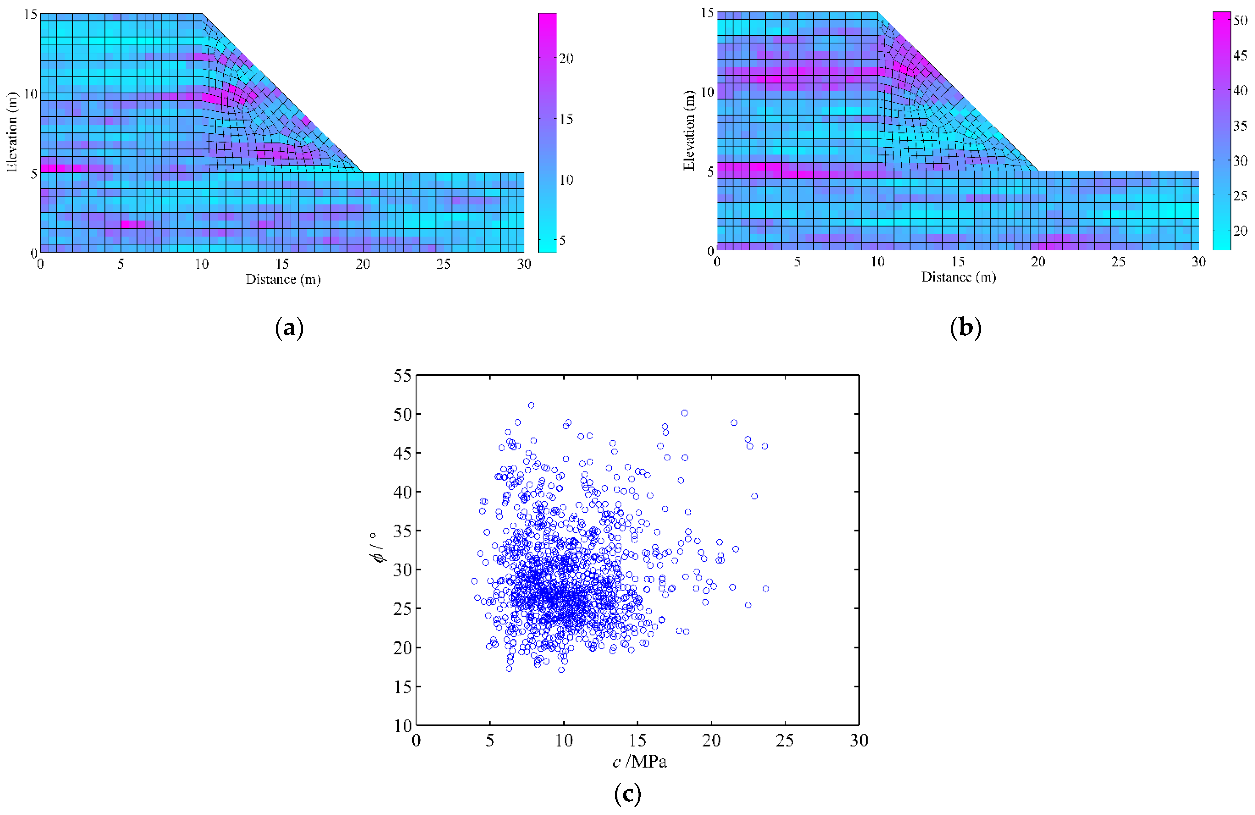
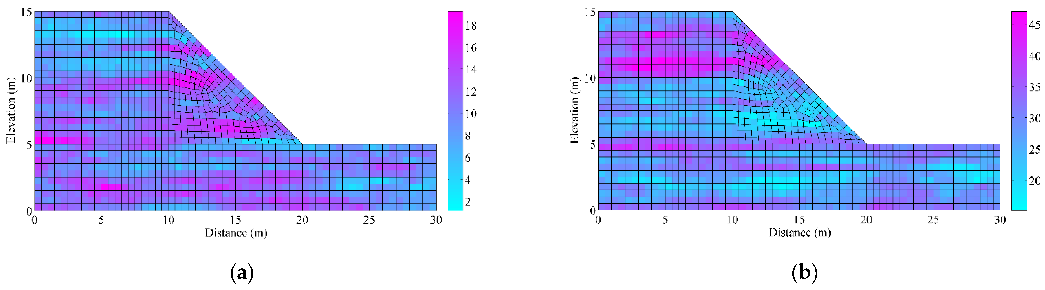
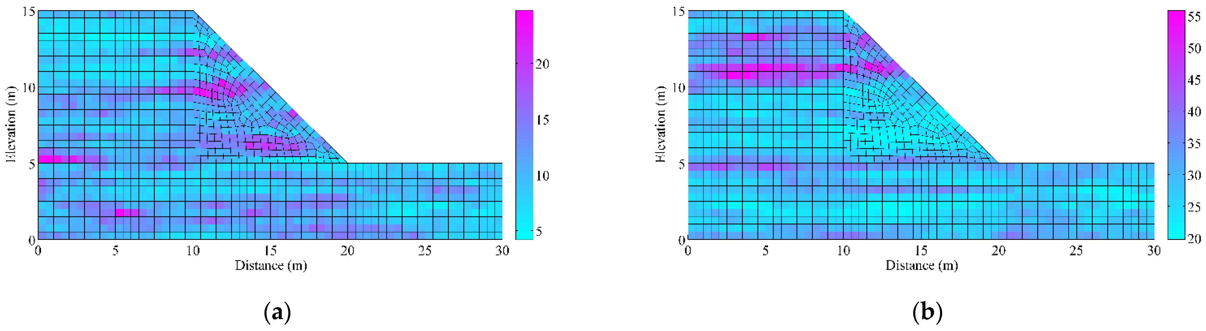
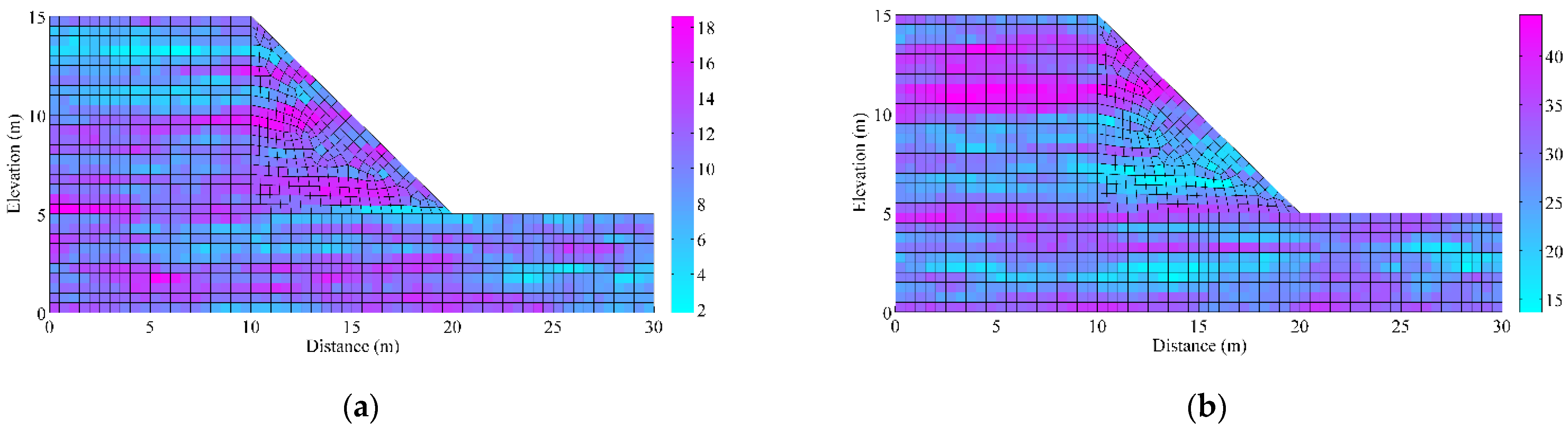
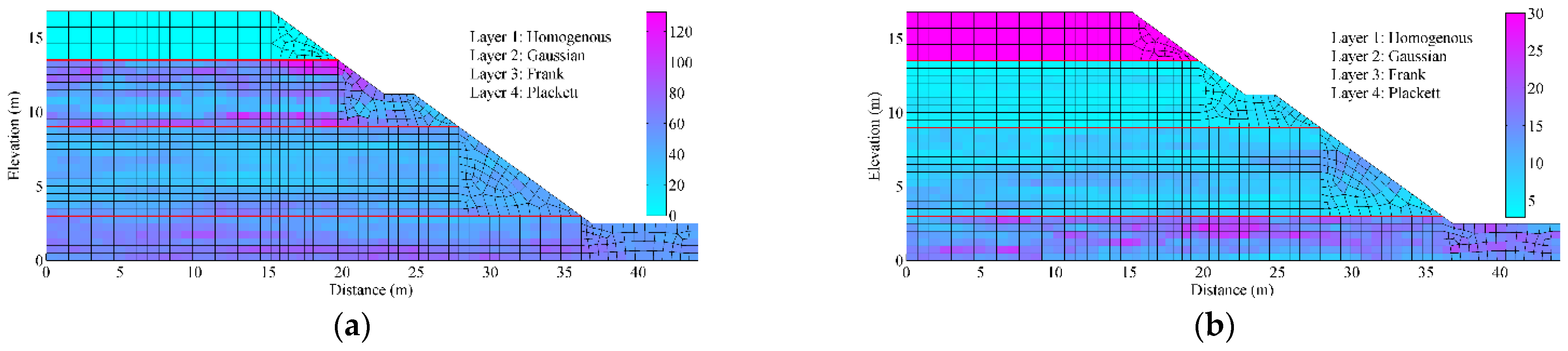
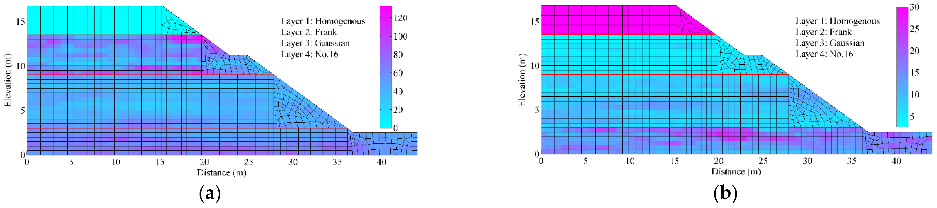
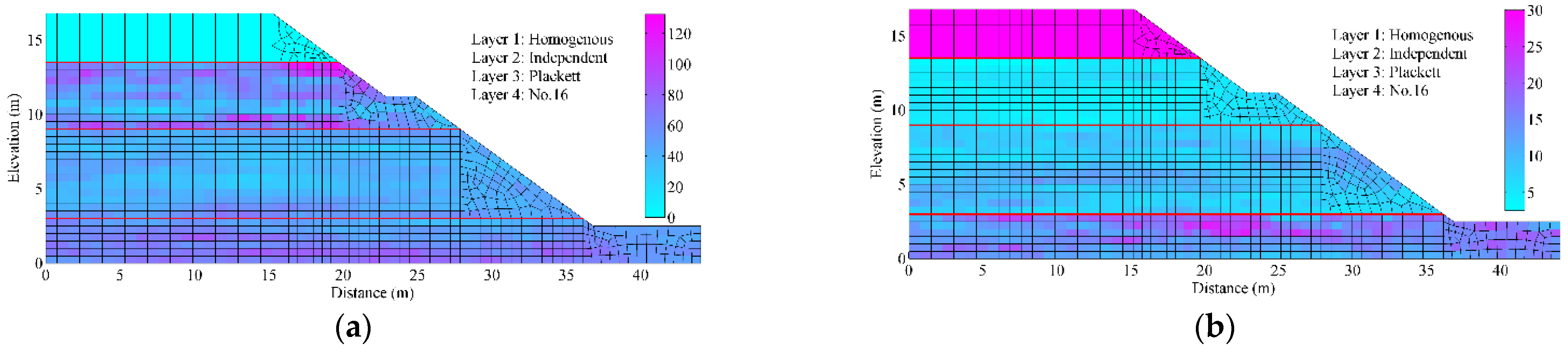
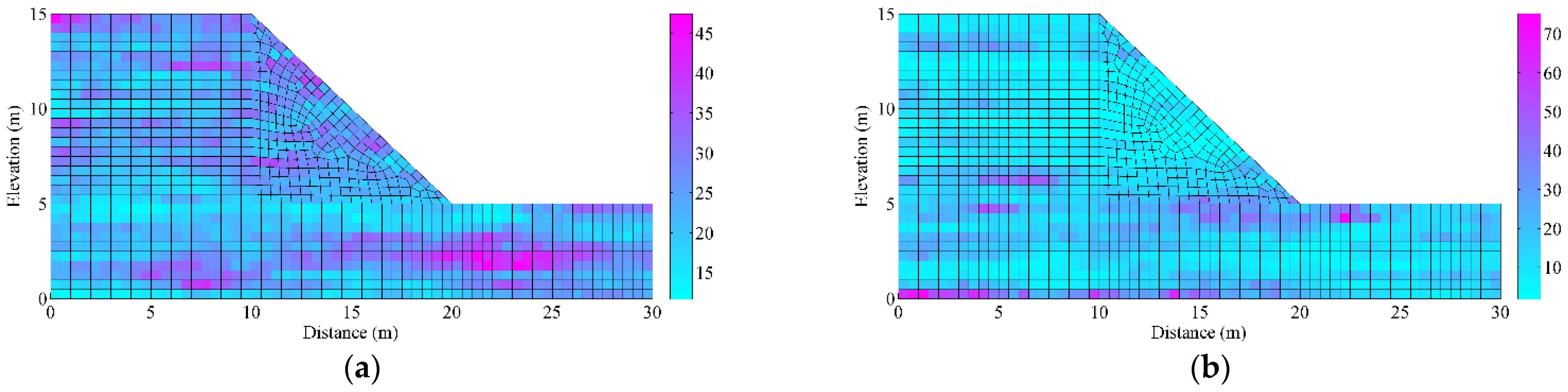
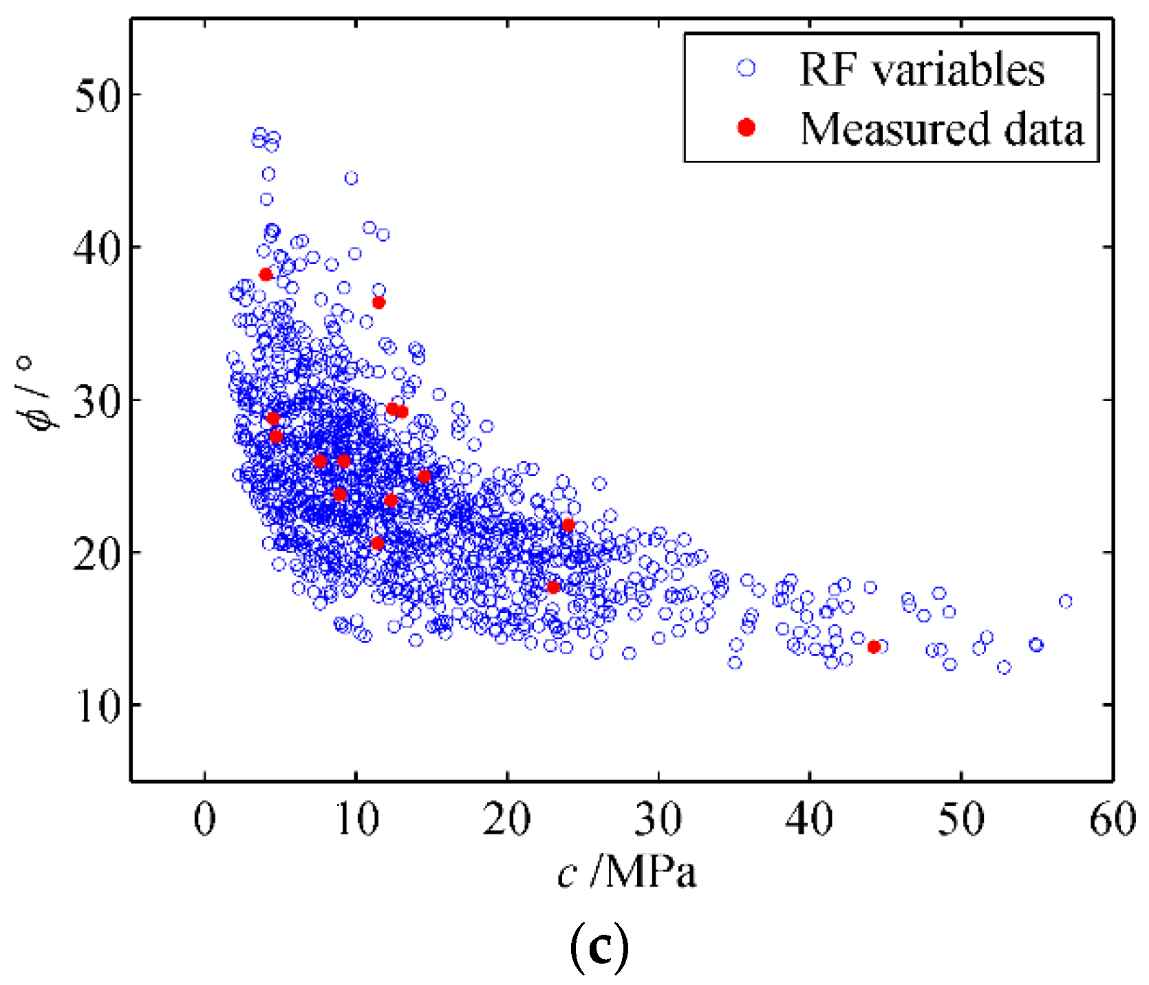
6.3.3. Simulation of CCRF for Soil Parameters
7. Conclusions
Author Contributions
Funding
Institutional Review Board Statement
Informed Consent Statement
Data Availability Statement
Conflicts of Interest
References
- Ali, A.; Huang, J.; Lyamin, A.V.; Sloan, S.W.; Griffiths, D.V.; Cassidy, M.J.; Li, J.H. Simplified quantitative risk assessment of rainfall-induced landslides modelled by infinite slopes. Eng. Geol. 2014, 179, 102–116. [Google Scholar] [CrossRef]
- Jiang, S.H.; Papaioannou, I.; Straub, D. Bayesian updating of slope reliability in spatially variable soils with in-situ measurements. Eng. Geol. 2018, 239, 310–320. [Google Scholar] [CrossRef]
- Liu, L.; Zhang, S.; Cheng, Y.M.; Liang, L. Advanced reliability analysis of slopes in spatially variable soils using multivariate adaptive regression splines. Geosci. Front. 2019, 10, 671–682. [Google Scholar] [CrossRef]
- Tang, X.S.; Wang, M.X.; Li, D.Q. Modeling multivariate cross-correlated geotechnical random fields using vine copulas for slope reliability analysis. Comput. Geotech. 2020, 127, 103784. [Google Scholar] [CrossRef]
- Wang, M.X.; Tang, X.S.; Li, D.Q.; Qi, X.H. Subset simulation for efficient slope reliability analysis involving copula-based cross-correlated random fields. Comput. Geotech. 2020, 118, 103326. [Google Scholar] [CrossRef]
- Dasaka, S.M. Probabilistic Site Characterization and Reliability Analysis of Shallow Foundations and Slopes. Ph.D. Dissertation, Indian Institute of Science, Bengaluru, India, 2005. [Google Scholar]
- Fenton, G.A.; Griffiths, D.V. Bearing-capacity prediction of spatially random c-ϕ soils. Can. Geotech. J. 2003, 40, 54–65. [Google Scholar] [CrossRef]
- Zhou, X.; Zhang, G.; Hu, S.; Li, J. Optimal estimation of shear strength parameters based on copula theory coupling information diffusion technique. Adv. Civ. Eng. 2019, 2019, 873869. [Google Scholar] [CrossRef] [Green Version]
- Zhou, X.; Zhang, G.; Hu, S.; Li, J.; Xuan, D.; Lv, C. Copula-based approach coupling information diffusion distribution for slope reliability analysis. Bull. Eng. Geol. Environ. 2020, 79, 2255–2270. [Google Scholar] [CrossRef]
- Dasgupta, U.S.; Chauhan, V.B.; Dasaka, S.M. Influence of spatially random soil on lateral thrust and failure surface in earth retaining walls. Georisk Assess. Manag. Risk Eng. Syst. Geohazards 2017, 11, 247–256. [Google Scholar] [CrossRef]
- Bayramoglu, I.; Gebizlioglu, O.L. A max–min model of random variables in bivariate random sequences. J. Comput. Appl. Math. 2021, 388, 113304. [Google Scholar] [CrossRef]
- Cheng, H.; Chen, J.; Chen, R.; Chen, G. Comparison of Modeling Soil Parameters Using Random Variables and Random Fields in Reliability Analysis of Tunnel Face. Int. J. Geomech. 2019, 19, 04018184. [Google Scholar] [CrossRef]
- Vanmarcke, E.H. Probabilistic modeling of soil profiles. J. Geotech. Eng. Div. 1977, 103, 1227–1246. [Google Scholar] [CrossRef]
- Zhang, L.; Li, D.Q.; Tang, X.S.; Cao, Z.J.; Phoon, K.K. Bayesian model comparison and characterization of bivariate distribution for shear strength parameters of soil. Comput. Geotech. 2018, 95, 110–118. [Google Scholar] [CrossRef]
- Tang, X.S.; Li, D.Q.; Zhou, C.B.; Phoon, K.K. Copula-based approaches for evaluating slope reliability under incomplete probability information. Struct. Saf. 2015, 52, 90–99. [Google Scholar] [CrossRef]
- Do, D.M.; Gao, K.; Yang, W.; Li, C.Q. Hybrid uncertainty analysis of functionally graded plates via multiple-imprecise-random-field modelling of uncertain material properties. Comput. Methods Appl. Mech. Eng. 2020, 368, 113116. [Google Scholar] [CrossRef]
- Yang, Z.; Li, X.; Qi, X. Efficient simulation of multivariate three-dimensional cross-correlated random fields conditioning on non-lattice measurement data. Comput. Methods Appl. Mech. Eng. 2022, 388, 114208. [Google Scholar] [CrossRef]
- Dasaka, S.M.; Zhang, L.M. Spatial variability of in situ weathered soil. Geotechnique 2012, 62, 375–384. [Google Scholar] [CrossRef] [Green Version]
- Napoli, M.L.; Barbero, M.; Ravera, E.; Scavia, C. A stochastic approach to slope stability analysis in bimrocks. Int. J. Rock Mech. Min. Sci. 2018, 101, 41–49. [Google Scholar] [CrossRef]
- Pandit, B.; Tiwari, G.; Latha, G.M.; Babu, G.L.S. Probabilistic Characterization of Rock Mass from Limited Laboratory Tests and Field Data: Associated Reliability Analysis and Its Interpretation. Rock Mech. Rock Eng. 2019, 52, 2985–3001. [Google Scholar] [CrossRef]
- Yang, R.; Huang, J.; Griffiths, D.V.; Sheng, D. Probabilistic stability analysis of slopes by conditional random fields. Geo-Risk 2017, 2017, 450–459. [Google Scholar] [CrossRef]
- Liu, Y.; Zhang, W.; Zhang, L.; Zhu, Z.; Hu, J.; Wei, H. Probabilistic stability analyses of undrained slopes by 3D random fields and finite element methods. Geosci. Front. 2018, 9, 1657–1664. [Google Scholar] [CrossRef]
- Jiang, S.H.; Huang, J.; Griffiths, D.V.; Deng, Z.P. Advances in reliability and risk analyses of slopes in spatially variable soils: A state-of-the-art review. Comput. Geotech. 2022, 141, 104498. [Google Scholar] [CrossRef]
- Zhu, H.; Zhang, L.M.; Xiao, T.; Li, X.Y. Generation of multivariate cross-correlated geotechnical random fields. Comput. Geotech. 2017, 86, 95–107. [Google Scholar] [CrossRef]
- Cho, S.E. Probabilistic Assessment of Slope Stability That Considers the Spatial Variability of Soil Properties. J. Geotech. Geoenviron. Eng. 2009, 136, 975–984. [Google Scholar] [CrossRef]
- Jiang, S.H.; Li, D.Q.; Zhang, L.M.; Zhou, C.B. Slope reliability analysis considering spatially variable shear strength parameters using a non-intrusive stochastic finite element method. Eng. Geol. 2014, 168, 120–128. [Google Scholar] [CrossRef]
- Nelsen, R.B. An Introduction to Copulas; Springer: New York, NY, USA, 2006. [Google Scholar]
- Nguyen, T.S.; Likitlersuang, S.; Tanapalungkorn, W.; Phan, T.N.; Keawsawasvong, S. Influence of copula approaches on reliability analysis of slope stability using random adaptive finite element limit analysis. Int. J. Numer. Anal. Met. 2022, 12, 46. [Google Scholar] [CrossRef]
- Wu, X.Z. Trivariate analysis of soil ranking-correlated characteristics and its application to probabilistic stability assessments in geotechnical engineering problems. Soils Found. 2013, 53, 540–556. [Google Scholar] [CrossRef] [Green Version]
- Wang, F.; Li, H. On the need for dependence characterization in random fields: Findings from cone penetration test (CPT) data. Can. Geotech. J. 2019, 56, 710–719. [Google Scholar] [CrossRef]
- Masoudian, M.S.; Hashemi Afrapoli, M.A.; Tasalloti, A.; Marshall, A.M. A general framework for coupled hydro-mechanical modelling of rainfall-induced instability in unsaturated slopes with multivariate random fields. Comput. Geotech. 2019, 115, 103162. [Google Scholar] [CrossRef]
- Griffiths, D.V.; Huang, J.; Fenton, G.A. Probabilistic infinite slope analysis. Comput. Geotech. 2011, 38, 577–584. [Google Scholar] [CrossRef]
- Savvas, D.; Papaioannou, I.; Stefanou, G. Bayesian identification and model comparison for random property fields derived from material microstructure. Comput. Methods Appl. Mech. Eng. 2020, 365, 113026. [Google Scholar] [CrossRef]
- Zheng, Z.; Dai, H. Simulation of multi-dimensional random fields by Karhunen–Loève expansion. Comput. Methods Appl. Mech. Eng. 2017, 324, 221–247. [Google Scholar] [CrossRef]
- Zhu, H. Probabilistic Evaluation and Field Testing of the Stability and Erodibility of Vegetated Slopes; The Hong Kong University of Science and Technology: Hongkong, China, 2014. [Google Scholar]
- Akaike, H. A New Look at the Statistical Model Identification. IEEE Trans. Automat. Contr. 1974, 19, 716–723. [Google Scholar] [CrossRef]
- Lan, W.; Wang, H.; Tsai, C.L. A Bayesian information criterion for portfolio selection. Comput. Stat. Data Anal. 2012, 56, 88–99. [Google Scholar] [CrossRef]
- Jiang, S.H.; Huang, J.S. Efficient slope reliability analysis at low-probability levels in spatially variable soils. Comput. Geotech. 2016, 75, 18–27. [Google Scholar] [CrossRef]
- Soenksen, P.J.; Turner, M.J.; Dietsch, B.J.; Simon, A. Stream Bank Stability in Eastern Nebraska; USGS Rep 03-4265; U.S. Geological Survey: Lincoln, NE, USA, 2003; p. 102.
- Smirnov, N. Table for Estimating the Goodness of Fit of Empirical Distributions. Ann. Math. Stat. 2007, 19, 279–281. [Google Scholar] [CrossRef]


| Copula | C(u,v; θ) | c(u,v; θ) | θ |
|---|---|---|---|
| Gaussian | [–1, 1] | ||
| Plackett | , | (0, +∞)\{1} | |
| Frank | (-∞, +∞)\{0} | ||
| No. 16 | , | , | [0, +∞) |
| Parameters | μ | COV | Margin | SOF | Cross-Correlation |
|---|---|---|---|---|---|
| c | 10 kPa | 0.3 | Lognormal | δh = 20 m, δv = 2 m | ρc,ϕ = −0.5 |
| ϕ | 30° | 0.2 | Lognormal | δh = 20 m, δv = 2 m |
| Parameter | Height | Slope Angle | Elastic Modulus | Poisson’s Ratio | Unit Weight |
|---|---|---|---|---|---|
| Value | 10 m | 45° | 35 MPa | 0.35 | 20 kN/m3 |
| Copulas | ρ | τ | μc | σc | COVc | μϕ | σϕ | COVϕ |
|---|---|---|---|---|---|---|---|---|
| Gaussian | −0.5031 | −0.3519 | 10.0787 | 3.0053 | 0.2982 | 29.9707 | 5.9839 | 0.1997 |
| Plackett | −0.4932 | −0.3739 | 10.0787 | 3.0053 | 0.2982 | 29.9686 | 5.9893 | 0.1999 |
| Frank | −0.4462 | −0.3326 | 10.0787 | 3.0053 | 0.2982 | 29.9658 | 5.9739 | 0.1994 |
| No.16 | −0.4879 | −0.4133 | 10.0787 | 3.0053 | 0.2982 | 29.8598 | 6.0121 | 0.2011 |
| Margins | ρ | τ | μc | σc | COVc | μϕ | σϕ | COVϕ |
|---|---|---|---|---|---|---|---|---|
| TN | −0.5238 | −0.3682 | 10.297 | 2.995 | 0.2909 | 28.918 | 6 | 0.2075 |
| TG | −0.4468 | −0.3682 | 10.293 | 3.132 | 0.3043 | 29.038 | 6.036 | 0.2079 |
| WB | −0.5266 | −0.3682 | 10.29 | 2.999 | 0.2915 | 28.893 | 6.003 | 0.2078 |
| LN and TN | −0.5181 | −0.3682 | 10.297 | 2.995 | 0.2909 | 28.963 | 6.024 | 0.2080 |
| Soil Layer | γ (kN/m3) | c (kPa) | ϕ (°) | ||||
|---|---|---|---|---|---|---|---|
| Margin | μc | COVc | Margin | μϕ | COVϕ | ||
| Sand layer 1 | 21.0 | - | 0 | - | - | - | |
| Clay layer 2 | 19.5 | LN | 55 | 0.37 | LN | 5 | 0.2 |
| Clay layer 3 | 19.5 | LN | 43 | 0.19 | LN | 7 | 0.21 |
| Clay layer 4 | 20.0 | LN | 56 | 0.20 | LN | 15 | 0.24 |
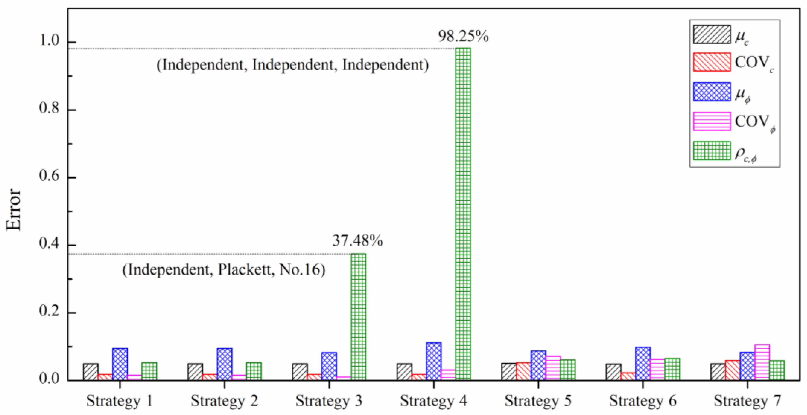
| Strategies | Margins | Copulas |
|---|---|---|
| Strategy 1 | (LN, LN) | (Gaussian, Frank, Plackett) |
| Strategy 2 | (LN, LN) | (Frank, Gaussian, No. 16) |
| Strategy 3 | (LN, LN) | (Independent, Plackett, No. 16) |
| Strategy 4 | (LN, LN) | (Independent, Independent, Independent) |
| Strategy 5 | (TN, TN) | (Gaussian, Frank, Plackett) |
| Strategy 6 | (TG, TG) | (Gaussian, Frank, Plackett) |
| Strategy 7 | (WB, WB) | (Gaussian, Frank, Plackett) |
| Copulas | Soil Layers | μc | COVc | μϕ | COVϕ | ρ |
|---|---|---|---|---|---|---|
| Strategy 1 | Layer 2 | 57.8521 | 0.3629 | 4.8705 | 0.2021 | −0.5091 |
| Layer 3 | 41.5108 | 0.1901 | 8.6453 | 0.2109 | −0.4383 | |
| Layer 4 | 59.4741 | 0.1931 | 15.3436 | 0.2321 | −0.5080 | |
| Strategy 2 | Layer 2 | 57.8521 | 0.3629 | 4.8747 | 0.2073 | −0.4639 |
| Layer 3 | 41.5108 | 0.1901 | 8.6081 | 0.2112 | −0.5181 | |
| Layer 4 | 59.4741 | 0.1931 | 15.0663 | 0.2375 | −0.5602 | |
| Strategy 3 | Layer 2 | 57.8521 | 0.3629 | 4.9316 | 0.1971 | −0.0244 |
| Layer 3 | 41.5108 | 0.1901 | 8.6091 | 0.2115 | −0.4735 | |
| Layer 4 | 59.4741 | 0.1931 | 15.0663 | 0.2375 | −0.5602 | |
| Strategy 4 | Layer 2 | 57.8521 | 0.3629 | 4.9316 | 0.1971 | −0.0244 |
| Layer 3 | 41.5108 | 0.1901 | 8.7082 | 0.2040 | −0.0098 | |
| Layer 4 | 59.4741 | 0.1931 | 16.1749 | 0.2279 | 0.0080 | |
| Strategy 5 | Layer 2 | 58.0809 | 0.3468 | 4.8671 | 0.2055 | −0.5254 |
| Layer 3 | 41.4723 | 0.1970 | 8.4923 | 0.1738 | −0.4457 | |
| Layer 4 | 59.4304 | 0.1885 | 15.3504 | 0.2365 | −0.5116 | |
| Strategy 6 | Layer 2 | 57.8589 | 0.3628 | 4.8763 | 0.1994 | −0.4954 |
| Layer 3 | 41.5646 | 0.1848 | 8.7449 | 0.2400 | −0.4179 | |
| Layer 4 | 59.4177 | 0.1955 | 15.3251 | 0.2299 | −0.4889 | |
| Strategy 7 | Layer 2 | 57.9215 | 0.3550 | 4.8668 | 0.2071 | −0.5243 |
| Layer 3 | 41.4660 | 0.2018 | 8.3971 | 0.1535 | −0.4396 | |
| Layer 4 | 59.3558 | 0.1849 | 15.3588 | 0.2365 | −0.5031 |
| Soil Parameters | Statistics | ||||
|---|---|---|---|---|---|
| μ | σ | COV | Pearson | Kendall | |
| c | 13.68 | 10.27 | 0.7511 | −0.716 | −0.4857 |
| ϕ | 25.85 | 6.36 | 0.2460 | ||
| Margins | c | ϕ | ||||
|---|---|---|---|---|---|---|
| Dn | AIC | BIC | Dn | AIC | BIC | |
| TN | 0.2682 | 112.58 | 114.00 | 0.1548 | 101.06 | 102.48 |
| LN | 0.1367 | 105.11 | 106.52 | 0.1237 | 101.71 | 103.12 |
| TG | 0.2164 | 108.03 | 109.45 | 0.1320 | 103.48 | 104.90 |
| WB | 0.1817 | 108.73 | 110.14 | 0.1688 | 101.44 | 102.85 |
| Copulas | Gaussian | Plackett | Frank | No. 16 |
|---|---|---|---|---|
| AIC | −6.2223 | −2.9015 | −3.3795 | 3.2895 |
| BIC | −5.5143 | −2.1934 | −2.6714 | 3.9976 |
| Margins | Copula | μc | COVc | μϕ | COVϕ | ρc,ϕ | τc,ϕ |
|---|---|---|---|---|---|---|---|
| (LN, LN) | Gaussian | 14.1232 | 0.7055 | 23.6476 | 0.2466 | −0.6255 | −0.4945 |
| (LN, LN) | Plackett | 14.1232 | 0.7055 | 23.4610 | 0.2513 | −0.5815 | −0.4755 |
| (LN, LN) | Frank | 14.1232 | 0.7055 | 23.5756 | 0.2527 | −0.5777 | −0.4855 |
| (LN, LN) | No.16 | 14.1232 | 0.7055 | 23.4873 | 0.2622 | −0.4617 | −0.3938 |
| (TN, TN) | Gaussian | 16.0378 | 0.5499 | 23.5136 | 0.2704 | −0.7000 | −0.4945 |
| (TG, TG) | Gaussian | 14.9426 | 0.6617 | 23.7249 | 0.2364 | −0.6355 | −0.4945 |
| (WB, WB) | Gaussian | 14.2407 | 0.7232 | 23.4831 | 0.2770 | −0.7033 | −0.4945 |
Disclaimer/Publisher’s Note: The statements, opinions and data contained in all publications are solely those of the individual author(s) and contributor(s) and not of MDPI and/or the editor(s). MDPI and/or the editor(s) disclaim responsibility for any injury to people or property resulting from any ideas, methods, instructions or products referred to in the content. |
© 2023 by the authors. Licensee MDPI, Basel, Switzerland. This article is an open access article distributed under the terms and conditions of the Creative Commons Attribution (CC BY) license (https://creativecommons.org/licenses/by/4.0/).
Share and Cite
Zhou, X.; Sun, Y.; Xiao, H. Simulation of Cross-Correlated Random Fields for Transversely Anisotropic Soil Slope by Copulas. Appl. Sci. 2023, 13, 4234. https://doi.org/10.3390/app13074234
Zhou X, Sun Y, Xiao H. Simulation of Cross-Correlated Random Fields for Transversely Anisotropic Soil Slope by Copulas. Applied Sciences. 2023; 13(7):4234. https://doi.org/10.3390/app13074234
Chicago/Turabian StyleZhou, Xinlong, Yueyang Sun, and Henglin Xiao. 2023. "Simulation of Cross-Correlated Random Fields for Transversely Anisotropic Soil Slope by Copulas" Applied Sciences 13, no. 7: 4234. https://doi.org/10.3390/app13074234