
ShuffleDetect: Detecting Adversarial Images against Convolutional Neural Networks


Abstract
:1. Introduction
2. CNNs and Adversarial Images
3. Related Works and Evaluation Criteria
- Detection rate (DR) represents the percentage of adversarial images that are correctly identified as such by the detector.
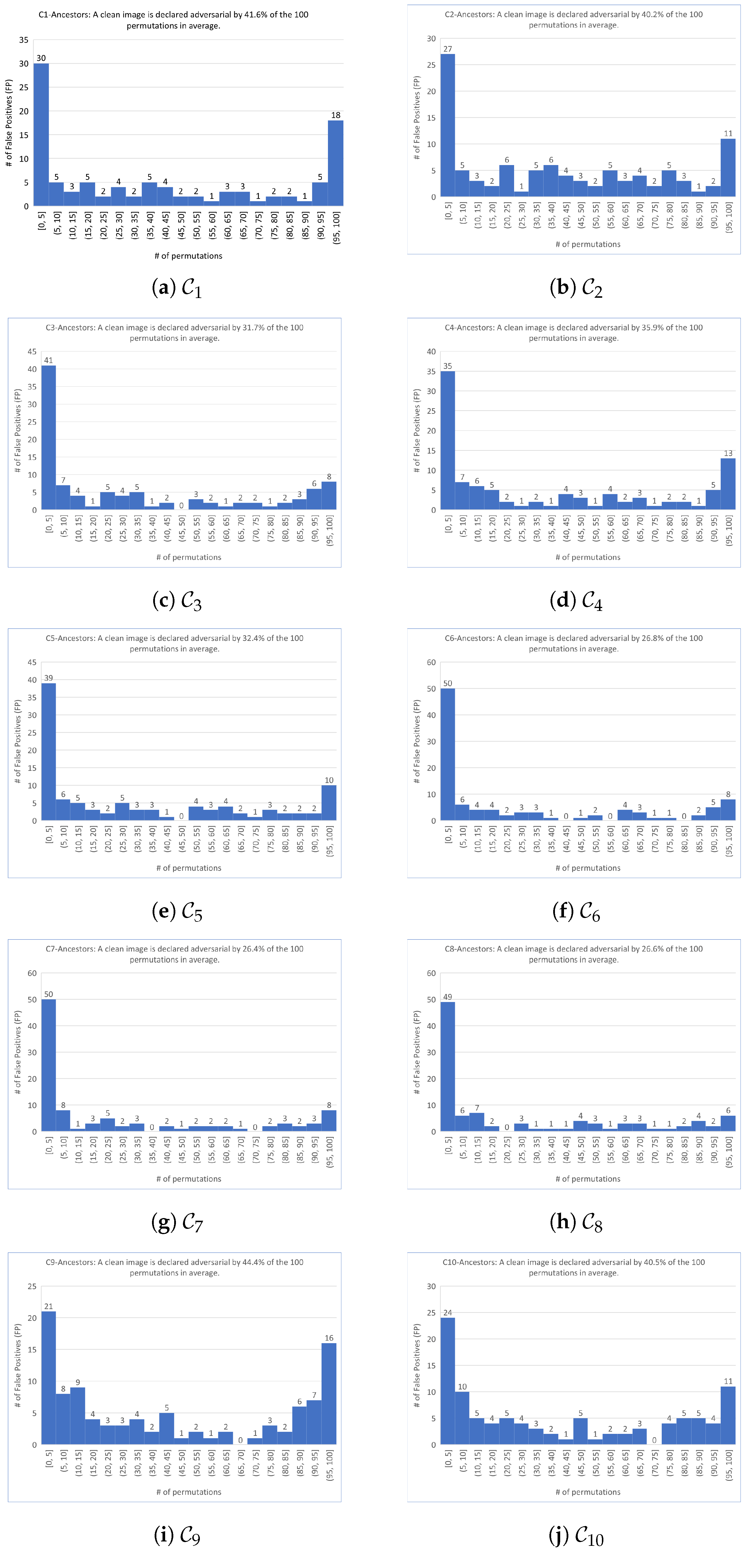
- False positive rate (FPR) represents the percentage of clean ancestor images that are identified as adversarial by the detector.
- Complexity refers to the time required to train a supervised detector.
- Overhead refers to the overall memory and computation resources necessary to use the detector (supervised or not). It depends on the number of parameters and size of the architecture of the detector, when applicable.
- Inference time latency is the amount of time required by the detector to run on an image. If the method is supervised, the inference time latency does not take into account the time needed to train the detector (this part is already taken into account in the Complexity measurements).
- Precision, Recall, and F1 scores used to quantify the detection performance are defined by the following formulae:where TP (true positive) is the number of correctly detected adversarial images, FN (false negative) is the number of adversarial images that escaped the detector, and FP (false positive) is the number of clean images declared adversarial by the detector. These formulae are pertinent whenever the number of clean images is equal to the number of adversarial images created by a given attack for a given CNN. This aspect is taken into account in Section 9.
4. ShuffleDetect
- as “adversarial” for if the output of is -adversarial for more than of the t permutations ,
- and as “clean” otherwise.
| Algorithm 1 pseudo-code |
|
5. The CNNs, the Scenarios, the Ancestor Images
6. The 8 Attacks
6.1. EA
6.2. FGSM
6.3. BIM
6.4. PGD Inf
6.5. PGD
6.6. PGD
6.7. CW Inf
6.8. DeepFool
7. The Adversarial Images Obtained by the 8 Attacks
8. Parameters and Experiments Performed on
9. Intrinsic Performance of
- matches the requirement that most permutations declare an image as adversarial.
- is motivated by the fact that the smallest among the 100 permutations and the four targeted attacks is .
- is motivated by the fact that the average of the among the 100 permutations and the four targeted attacks is .
- as a demanding ratio compromise.
- for the same reason as for the target case.
- because it makes sense to keep the same demanding value for the detector independently on the scenario of the attack, hence the same value for the targeted attack.
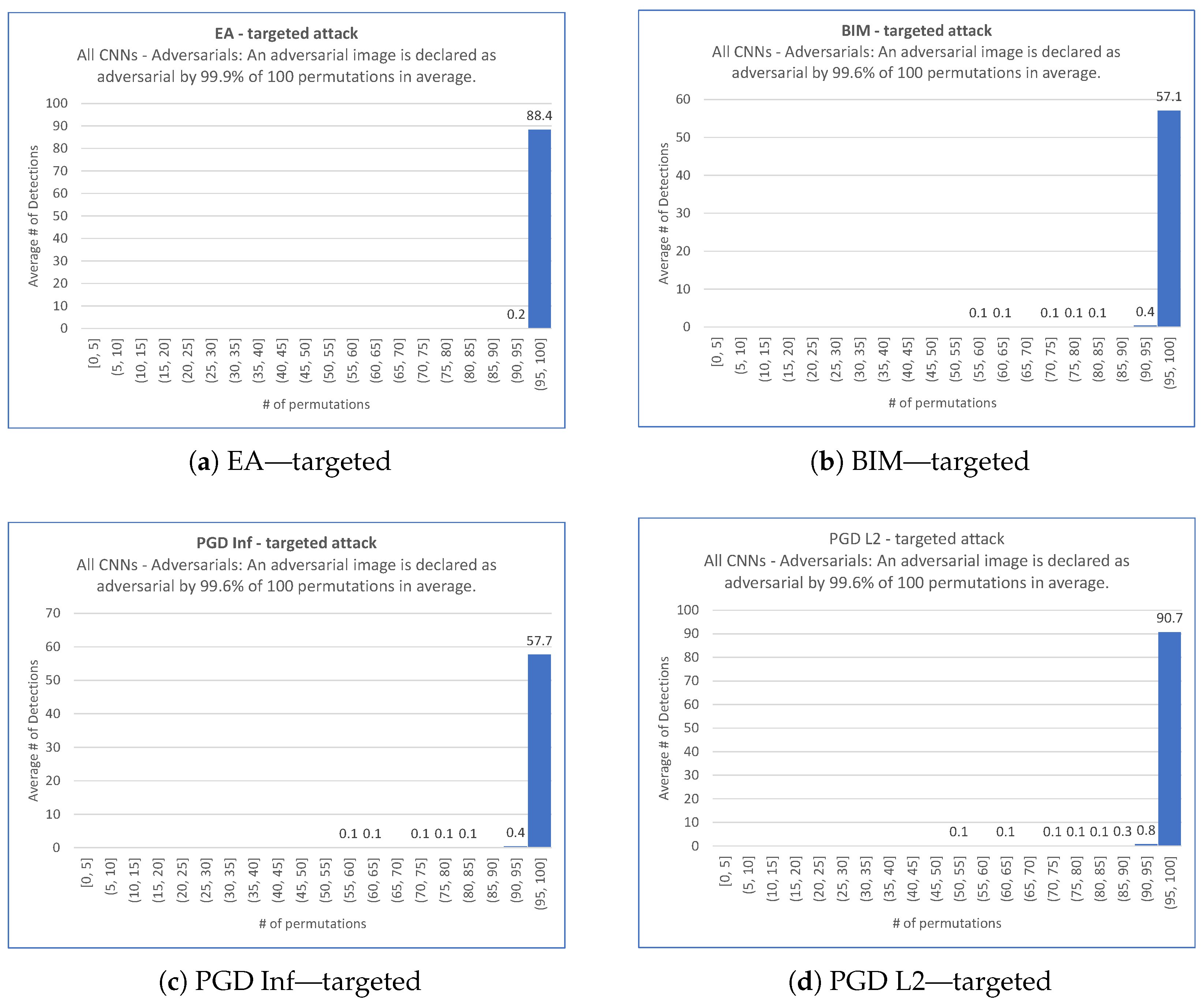
- For all targeted attacks, the detection rate is , the value is , and the average values of these indicators are and , respectively.
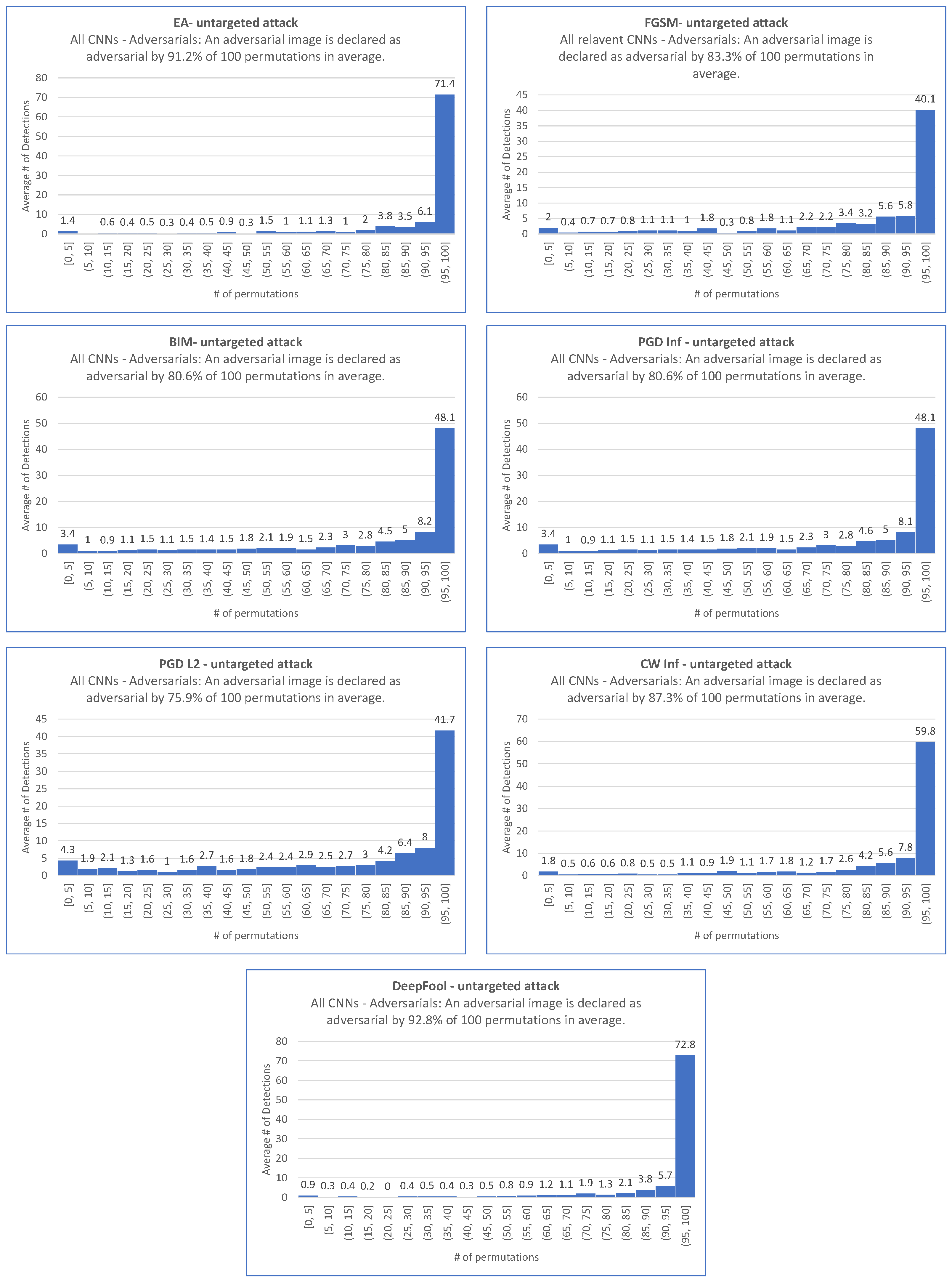
- For untargeted attacks, the detection rate is , the value is , and the average values are and , respectively.
10. Performance Comparison of ShuffleDetect and Feature Squeezer (FS)
- Color depth reduction: the image color depth is decreased to 5 bits.
- Median smoothing: the filter size is set to .
- Non-local means: the search window size is set to , the patch size is set to , and the filter strength is set to 4.
- The threshold is set to .
11. Conclusions
Author Contributions
Funding
Institutional Review Board Statement
Informed Consent Statement
Data Availability Statement
Acknowledgments
Conflicts of Interest
Appendix A


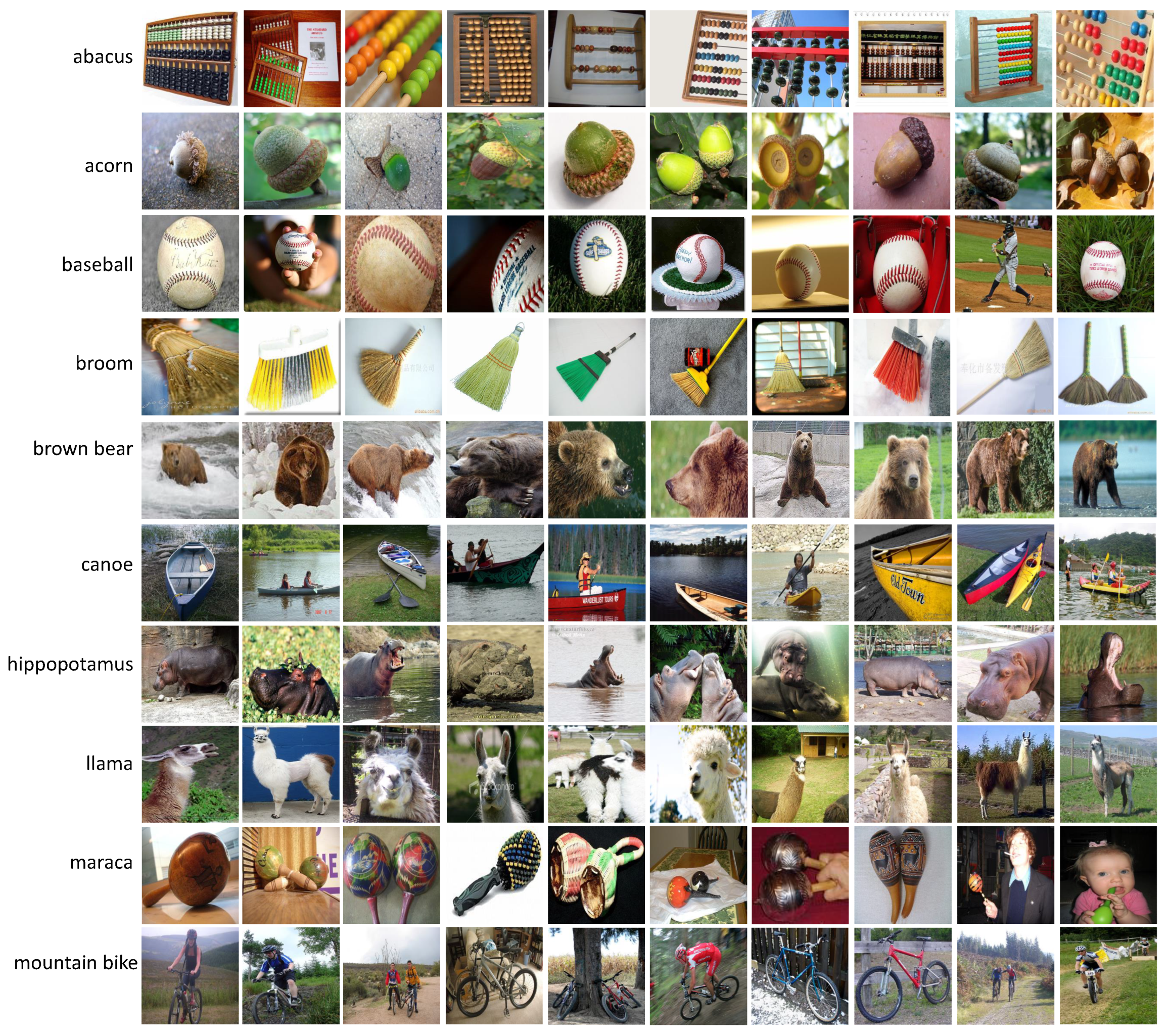
| Ancestor Images and Their Original Size | ||||||||||||
|---|---|---|---|---|---|---|---|---|---|---|---|---|
| 1 | 2 | 3 | 4 | 5 | 6 | 7 | 8 | 9 | 10 | |||
| abacus | 1 | (206, 250) | (960, 1280) | (262, 275) | (598, 300) | (377, 500) | (501, 344) | (375, 500) | (448, 500) | (500, 500) | (150, 200) | |
| acorn | 2 | (374, 500) | (500, 469) | (375, 500) | (500, 375) | (500, 500) | (500, 500) | (375, 500) | (374, 500) | (461, 500) | (333, 500) | |
| baseball | 3 | (398, 543) | (240, 239) | (180, 240) | (333, 500) | (262, 350) | (310, 310) | (404, 500) | (344, 500) | (375, 500) | (285, 380) | |
| broom | 4 | (113, 160) | (150, 150) | (333, 500) | (500, 333) | (497, 750) | (336, 500) | (188, 250) | (375, 500) | (334, 500) | (419, 640) | |
| brown bear | 5 | (500, 333) | (286, 490) | (360, 480) | (298, 298) | (413, 550) | (366, 500) | (400, 400) | (348, 500) | (346, 500) | (640, 480) | |
| canoe | 6 | (500, 332) | (450, 600) | (500, 375) | (375, 500) | (406, 613) | (600, 400) | (1067, 1600) | (333, 500) | (1536, 2048) | (375, 500) | |
| hippopotamus | 7 | (375, 500) | (1200, 1600) | (333, 500) | (450, 291) | (525, 525) | (375, 500) | (500, 457) | (424, 475) | (500, 449) | (339, 500) | |
| llama | 8 | (500, 333) | (618, 468) | (500, 447) | (253, 380) | (500, 333) | (333, 500) | (375, 500) | (375, 500) | (290, 345) | (375, 500) | |
| maraca | 9 | (375, 500) | (375, 500) | (470, 627) | (151, 220) | (250, 510) | (375, 500) | (99, 104) | (375, 500) | (375, 500) | (500, 375) | |
| mountain bike | 10 | (375, 500) | (500, 375) | (375, 500) | (333, 500) | (500, 375) | (300, 402) | (375, 500) | (446, 500) | (375, 500) | (500, 333) | |
Appendix B
| Left Grid | Right Grid | ||||||
|---|---|---|---|---|---|---|---|
| t = 100 | |||
|---|---|---|---|
| Round | Permutation | Round | Permutation |
| 1 | (1,13,4,6)(2,14,10)(3,11,12,5,9)(7,16,15,8) | 51 | (1,9,10,8,13,6,2,15,5,14,4,7,11)(3,16) |
| 2 | (1,8,9,2,6,11,15,12)(3,4,5,10,7)(14,16) | 52 | (1,11,15,4,10,2,3,5,12,9,13,8,16,7)(6,14) |
| 3 | (1,2,10,12)(3,11,16,15)(4,6,13,7,14,9,5) | 53 | (1,12,3,7,2,5,6,15,16,14,4,10)(8,13)(9,11) |
| 4 | (1,12,7,6,9,5,13,16)(2,4,14,10)(3,11,15,8) | 54 | (1,2,13,12,7)(3,6,4,8)(9,10)(11,15) |
| 5 | (3,5,14,16,7,4,12,6,13,11)(8,15,9,10) | 55 | (1,6,3)(2,12,14,4,15,7)(5,9)(8,13,10,11,16) |
| 6 | (1,7,4,9,2,5)(3,14)(6,16,8,13,10,15,12,11) | 56 | (1,8,3,4,13,10,9,16,5,2,7,11,12)(6,15) |
| 7 | (1,7,15,5,10,4,2,13,14,12,6,9)(3,11,16,8) | 57 | (1,5,12,9,15,4,7,11,2,10,6,16,8,3,14) |
| 8 | (1,2,5)(3,11,16,10,12,9,7,6,15,4,13,8) | 58 | (1,12)(2,6,13,10,7,8)(3,15,5,16,11,9)(4,14) |
| 9 | (1,7,15,8,13,5,9,11)(2,12)(3,16,14,4)(6,10) | 59 | (2,11,13,6)(3,12,10,7,16,4)(5,8)(9,15,14) |
| 10 | (1,16,8,15,4,5,6)(3,14,13)(7,12)(9,10,11) | 60 | (1,13,15,8,4,14,5,9,12,7,10,11,16,3,6,2) |
| 11 | (1,8,10,13,9,6,2)(3,12,5,15,14,4,7)(11,16) | 61 | (1,2,14,6,10,7)(4,5,12,9,8,16,11) |
| 12 | (1,4,14,16,5,6,11,13,15,9)(2,12,10,3,8) | 62 | (1,11)(2,7,4,5,10,12,14,9)(3,6,8,13,15,16) |
| 13 | (1,5,14,13,10)(2,6,7,4,8)(3,15,11,9,16,12) | 63 | (1,9,14,15,11,5,8,10,2,4,3,12,16,13,6,7) |
| 14 | (1,16,9,4,3,2,5,7,6,11,12,10,8,15,14,13) | 64 | (2,11,12,10,5)(3,16,14,13,4,8,6,15)(7,9) |
| 15 | (1,16,5,13,8,6)(2,15,14,10,11,12,9,3,7,4) | 65 | (1,5,12,3,2,6,11,13,16,14)(7,10,15) |
| 16 | (1,14,12,2,13,7,10,8,3,15,11,6,16,4) | 66 | (1,15,7,11,12,2)(3,10,4,14,5,8,6,16,9,13) |
| 17 | (1,2,5,13)(4,11,8,10,16,14,15)(6,7)(9,12) | 67 | (1,4)(2,6,15,11,12,16)(3,5,14)(7,8)(9,10) |
| 18 | (1,12,13,16,3,8,10,2,11,14,7,4,15,6) | 68 | (1,13,6,14,2,10,5,15,11,9,4,12,8,3,7,16) |
| 19 | (1,8,4,16,3,13,6,7,15)(2,12)(5,14,11)(9,10) | 69 | (1,9,15,6,8,10,11,2,12,16,4,13,14,7)(3,5) |
| 20 | (1,14,15,5)(2,4,12,13)(3,8,16,11)(6,7)(9,10) | 70 | (1,2,6,8,3)(4,12)(5,7,13,10,15)(9,11,14,16) |
| 21 | (1,2,6)(3,8,14,10,13,12)(5,9,16,15) | 71 | (2,10,16,6,13,3,14,12)(4,5,8,15,7,9,11) |
| 22 | (1,3,11,14,2,10)(4,12,6,7,15,5,16,9)(8,13) | 72 | (1,8,13,7)(2,10,15,6,14,9,3,16,5,11) |
| 23 | (1,4,11,9,14,7,2,5,3,8,6)(10,15) | 73 | (1,5,16,12,6,2,8,11,4,10,9,13,14)(7,15) |
| 24 | (1,12,8,7)(2,4,5,14,6,9,3,13,16)(10,15,11) | 74 | (1,6,16,13,11,5,14,4,3,9,15,2,8,10,7) |
| 25 | (1,14,6,4,10,16,5,13,12,2,8,15,9,3,7,11) | 75 | (1,12,9,6,15,4,5,14,2,3)(7,11,16)(8,13) |
| 26 | (1,15,5)(2,13,4,9,16,8,11,12,3,6,10,14,7) | 76 | (1,11,15,16,9)(2,12,5,3,8,13,6)(7,10,14) |
| 27 | (1,10,8,12,14,7,2)(3,13,11,5,6)(4,15) | 77 | (2,8,15,10,16,9,12,7,4)(3,5,11,14)(6,13) |
| 28 | (1,8,11,7,16,5,6,12,4,14)(2,15,3,10,9) | 78 | (1,15,11,8,16,5,2,12,3,13,6,10,14)(4,9) |
| 29 | (1,5,3,12,15,11)(2,14,10,6,8,9,7,13,16) | 79 | (1,16,13,5,3,10,6,4,15,2,11)(7,14,9) |
| 30 | (1,10,8,15)(3,9,7,4,12)(5,11,6) | 80 | (2,10,13,11,15,6,5,8,3,16,4,7,9,14) |
| 31 | (1,3,10,6,9,7,16,2,8)(4,5,14)(12,13) | 81 | (1,5,15,2,16,10,9,14,11,4,12,6,3) |
| 32 | (1,2,11,16,10,15)(3,14,6,5,9)(4,7,13,12) | 82 | (1,13,5,10,2,15,11,4,16,7,12,9,14,3,8,6) |
| 33 | (1,16,14,13,10,7,12,3,6,11,9,5)(2,4) | 83 | (1,14,8,9,15,3,5,2,7,10,4,12,6,11,16) |
| 34 | (1,6,14)(2,10,3,15,9,12,11,4,16,13,8,7) | 84 | (1,15,8,9,4,3,16,6,7,14,5,12,2,10,13,11) |
| 35 | (1,2)(3,15,16,13,12,4,5,6,7,9,10,11)(8,14) | 85 | (1,9,3,13)(4,11,15,12)(5,16,6,10,7,8,14) |
| 36 | (3,12,8,6,7,10,16,5,15,13)(4,9) | 86 | (1,9,15,8,13,14,6,11,7)(2,10,12,3,16,5,4) |
| 37 | (1,3,10,4,15,8,16,12,13,7,14,9,2) | 87 | (1,3,9,7,6,4,5)(10,12,14,16,11)(13,15) |
| 38 | (1,4,16)(2,9,5,13,10,14,3,11,8,7)(12,15) | 88 | (1,9,8,12,14,5,10,6,15,4,3)(2,11,16,13) |
| 39 | (1,4,5,2,11,10,12,9,14,15,3,16,13)(7,8) | 89 | (1,13,2,9,16)(3,14,11,8,7,15,6)(5,12,10) |
| 40 | (1,9,8,15,5,10,11,12,4,14,2,3,13,16,6,7) | 90 | (1,8,16,2,6,3,10,14,7,13,4,9,12,5,11) |
| 41 | (1,8,9,11,16,4)(2,13,14,15,7,12)(3,10,5) | 91 | (1,5,16,6,10,3,11,15,9,12,14,8,7,2,4) |
| 42 | (1,9,4,15,14,5)(2,11,12,3,6,10,13)(7,8,16) | 92 | (1,10,16,11,4,8,5,12,13,3,14,9)(2,7,15) |
| 43 | (2,8,14,9,7,16,12,10,13,6,15,3,11,4,5) | 93 | (1,4,2,13,6,9,14,3,10,8,16,11,15,7) |
| 44 | (1,11,12,14,2,13,8,9,3,10,6)(5,15,16) | 94 | (1,16,15,3,9,2,6,7,11,4)(5,8,14,12)(10,13) |
| 45 | (1,3,16,4)(2,5,6,15,7,11)(8,9,10)(13,14) | 95 | (3,10,13,15,12,9,14,16,7,5,4,6,8,11) |
| 46 | (1,6,12,10,8,15,5)(2,4,16,3,13)(7,14,9,11) | 96 | (1,6,15,4,5,3,16,13,9,10,12,2,8,7) |
| 47 | (1,7,14,3,4,16,8,13)(2,9)(5,12,6,11)(10,15) | 97 | (1,14,2,7,3,13,8,16,5,11,15,4,6,10,9,12) |
| 48 | (1,8,14,6,11,13,3,10,12,16,2,15,5,7,4) | 98 | (1,13,3,16)(2,11,6,14,5)(4,9,10,7,12,8,15) |
| 49 | (1,8,12,10,11,6,9,15)(3,13,4,7)(5,16,14) | 99 | (1,6,13,5,12,15,2)(3,14,8)(7,11)(9,16,10) |
| 50 | (1,5,16,2,11,4,13,15,12,3,8,7,14,6) | 100 | (1,12,11,8,2,3)(4,14,16,7,10,6)(5,13,15) |
| Per Permutation | |||||
|---|---|---|---|---|---|
| Steps: 8–12 | Shuffling | Predicting | Shuff% | Pred% | |
| Step: 8 | Steps: 9–10 | ||||
| 0.0955 | 0.0014 | 0.0941 | 1.483 | 98.511 | |
| 0.1176 | 0.0014 | 0.1162 | 1.228 | 98.767 | |
| 0.0578 | 0.0016 | 0.0563 | 2.727 | 97.264 | |
| 0.0933 | 0.0016 | 0.0917 | 1.664 | 98.330 | |
| 0.1262 | 0.0016 | 0.1246 | 1.233 | 98.763 | |
| 0.0660 | 0.0016 | 0.0644 | 2.449 | 97.542 | |
| 0.0844 | 0.0017 | 0.0828 | 1.975 | 98.018 | |
| 0.1017 | 0.0017 | 0.1000 | 1.678 | 98.316 | |
| 0.0213 | 0.0015 | 0.0198 | 6.930 | 93.047 | |
| 0.0196 | 0.0015 | 0.0182 | 7.563 | 92.411 | |
| AVG | 0.0784 | 0.0015 | 0.077 | 1.978 | 98.015 |
Appendix C


References
- Touvron, H.; Cord, M.; Douze, M.; Massa, F.; Sablayrolles, A.; Jégou, H. Training data-efficient image transformers & distillation through attention. In Proceedings of the International Conference on Machine Learning, PMLR, Virtual, 18–24 July 2021; pp. 10347–10357. [Google Scholar]
- Chakraborty, A.; Alam, M.; Dey, V.; Chattopadhyay, A.; Mukhopadhyay, D. Adversarial Attacks and Defences: A Survey. arXiv 2018, arXiv:1810.00069. [Google Scholar] [CrossRef]
- Kurakin, A.; Goodfellow, I.J.; Bengio, S. Adversarial examples in the physical world. In Artificial Intelligence Safety and Security; Chapman and Hall/CRC: Boca Raton, FL, USA, 2018; pp. 99–112. [Google Scholar]
- Goodfellow, I.J.; Shlens, J.; Szegedy, C. Explaining and Harnessing Adversarial Examples. arXiv 2015, arXiv:1810.00069. [Google Scholar]
- Carlini, N.; Wagner, D. Towards evaluating the robustness of neural networks. In Proceedings of the 2017 IEEE Symposium on Security and Privacy (SP), IEEE, San Jose, CA, USA, 22–26 May 2017; pp. 39–57. [Google Scholar]
- Wiyatno, R.; Xu, A. Maximal Jacobian-based Saliency Map Attack. arXiv 2018, arXiv:1808.07945. [Google Scholar]
- Tramèr, F.; Papernot, N.; Goodfellow, I.; Boneh, D.; McDaniel, P. The Space of Transferable Adversarial Examples. arXiv 2017, arXiv:1704.03453. [Google Scholar]
- Liu, Y.; Chen, X.; Liu, C.; Song, D. Delving into Transferable Adversarial Examples and Black-box Attacks. arXiv 2016, arXiv:1611.02770. [Google Scholar]
- Ilyas, A.; Engstrom, L.; Athalye, A.; Lin, J. Black-box adversarial attacks with limited queries and information. In Proceedings of the International Conference on Machine Learning, PMLR, Stockholm, Sweden, 10–15 July 2018; pp. 2137–2146. [Google Scholar]
- Narodytska, N.; Kasiviswanathan, S.P. Simple Black-Box Adversarial Perturbations for Deep Networks. arXiv 2016, arXiv:1612.06299. [Google Scholar]
- Feinman, R.; Curtin, R.R.; Shintre, S.; Gardner, A.B. Detecting adversarial samples from artifacts. arXiv 2017, arXiv:1703.00410. [Google Scholar]
- Grosse, K.; Manoharan, P.; Papernot, N.; Backes, M.; McDaniel, P. On the (statistical) detection of adversarial examples. arXiv 2017, arXiv:1702.06280. [Google Scholar]
- Xu, W.; Evans, D.; Qi, Y. Feature Squeezing: Detecting Adversarial Examples in Deep Neural Networks. arXiv 2017, arXiv:1704.01155. [Google Scholar]
- Liang, B.; Li, H.; Su, M.; Li, X.; Shi, W.; Wang, X. Detecting adversarial image examples in deep neural networks with adaptive noise reduction. IEEE Trans. Dependable Secure Comput. 2018, 18, 72–85. [Google Scholar] [CrossRef] [Green Version]
- Van Rossum, G.; Drake, F.L. Python 3 Reference Manual; CreateSpace: Scotts Valley, CA, USA, 2009. [Google Scholar]
- Oliphant, T.E. A Guide to NumPy; Trelgol Publishing: Austin, TX, USA, 2006. [Google Scholar]
- Paszke, A.; Gross, S.; Massa, F.; Lerer, A.; Bradbury, J.; Chanan, G.; Killeen, T.; Lin, Z.; Gimelshein, N.; Antiga, L.; et al. Pytorch: An imperative style, high-performance deep learning library. Adv. Neural Inf. Process. Syst. 2019, 32, 8026–8037. [Google Scholar]
- Varrette, S.; Bouvry, P.; Cartiaux, H.; Georgatos, F. Management of an Academic HPC Cluster: The UL Experience. In Proceedings of the 2014 International Conference on High Performance Computing & Simulation (HPCS 2014), IEEE, Bologna, Italy, 21–25 July 2014; pp. 959–967. [Google Scholar]
- Topal, A.O.; Chitic, R.; Leprévost, F. One evolutionary algorithm deceives humans and ten convolutional neural networks trained on ImageNet at image recognition. ASC, 2022; under review. [Google Scholar]
- Aldahdooh, A.; Hamidouche, W.; Fezza, S.A.; Déforges, O. Adversarial example detection for DNN models: A review and experimental comparison. Artif. Intell. Rev. 2022, 55, 4403–4462. [Google Scholar] [CrossRef]
- Ma, X.; Li, B.; Wang, Y.; Erfani, S.M.; Wijewickrema, S.N.R.; Houle, M.E.; Schoenebeck, G.; Song, D.; Bailey, J. Characterizing Adversarial Subspaces Using Local Intrinsic Dimensionality. arXiv 2018, arXiv:1801.02613. [Google Scholar]
- Ma, S.; Liu, Y. Nic: Detecting adversarial samples with neural network invariant checking. In Proceedings of the 26th Network and Distributed System Security Symposium (NDSS 2019), San Diego, CA, USA, 24–27 February 2019. [Google Scholar]
- Chitic, R.; Topal, A.O.; Leprévost, F. Empirical Perturbation Analysis of Two Adversarial Attacks: Black Box versus White Box. Appl. Sci. 2022, 12, 7339. [Google Scholar] [CrossRef]
- Leprévost, F. How Big is Big? How Fast is Fast? A Hands—On Tutorial on Mathematics of Computation; Amazon: New York, NY, USA, 2020. [Google Scholar]
- Deng, J.; Dong, W.; Socher, R.; Li, L.J.; Li, K.; Li, F.-F. The ImageNet Image Database. 2009. Available online: http://image-net.org (accessed on 20 September 2022).
- Simonyan, K.; Zisserman, A. Very deep convolutional networks for large-scale image recognition. arXiv 2014, arXiv:1409.1556. [Google Scholar]
- He, K.; Zhang, X.; Ren, S.; Sun, J. Deep residual learning for image recognition. In Proceedings of the IEEE Conference on Computer Vision and Pattern Recognition, Las Vegas, NV, USA, 26 June–1 July 2016; pp. 770–778. [Google Scholar]
- Huang, G.; Liu, Z.; Van Der Maaten, L.; Weinberger, K.Q. Densely connected convolutional networks. In Proceedings of the IEEE Conference on Computer Vision and Pattern Recognition, Honolulu, HI, USA, 21–26 July 2017; pp. 4700–4708. [Google Scholar]
- Howard, A.G.; Zhu, M.; Chen, B.; Kalenichenko, D.; Wang, W.; Weyand, T.; Andreetto, M.; Adam, H. Mobilenets: Efficient convolutional neural networks for mobile vision applications. arXiv 2017, arXiv:1704.04861. [Google Scholar]
- Tan, M.; Chen, B.; Pang, R.; Vasudevan, V.; Le, Q.V. MnasNet: Platform-Aware Neural Architecture Search for Mobile. arXiv 2018, arXiv:1807.11626. [Google Scholar]
- Agrafiotis, D. Chapter 9—Video Error Concealment. In Academic Press Library in Signal Processing; Theodoridis, S., Chellappa, R., Eds.; Elsevier: Amsterdam, The Netherlands, 2014; Volume 5, pp. 295–321. [Google Scholar] [CrossRef]
- Nicolae, M.; Sinn, M.; Minh, T.N.; Rawat, A.; Wistuba, M.; Zantedeschi, V.; Molloy, I.M.; Edwards, B. Adversarial Robustness Toolbox v1.0.0. arXiv 2018, arXiv:1807.01069. [Google Scholar]
- Madry, A.; Makelov, A.; Schmidt, L.; Tsipras, D.; Vladu, A. Towards Deep Learning Models Resistant to Adversarial Attacks. arXiv 2019, arXiv:1706.06083. [Google Scholar]
- Moosavi-Dezfooli, S.M.; Fawzi, A.; Frossard, P. Deepfool: A simple and accurate method to fool deep neural networks. In Proceedings of the IEEE Conference on Computer Vision and Pattern Recognition, Las Vegas, NV, USA, 26 June–1 July 2016; pp. 2574–2582. [Google Scholar]
- Meng, D.; Chen, H. Magnet: A two-pronged defense against adversarial examples. In Proceedings of the 2017 ACM SIGSAC Conference on Computer and Communications Security, Abu Dhabi, United Arab Emirates, 2–6 April 2017; pp. 135–147. [Google Scholar]


| p | ||
|---|---|---|
| 1 | (abacus, 398) | (bannister, 421) |
| 2 | (acorn, 988) | (rhinoceros beetle, 306) |
| 3 | (baseball, 429) | (ladle, 618) |
| 4 | (broom, 462) | (dingo, 273) |
| 5 | (brown bear, 294) | (pirate, 724) |
| 6 | (canoe, 472) | (saluki, 176) |
| 7 | (hippopotamus, 344) | (trifle, 927) |
| 8 | (llama, 355) | (agama, 42) |
| 9 | (maraca, 641) | (conch, 112) |
| 10 | (mountain bike, 671) | (strainer, 828) |
| Total | |||||||||||
|---|---|---|---|---|---|---|---|---|---|---|---|
| EA | (96, 91) | (97, 90) | (99, 88) | (98, 84) | (98, 79) | (99, 85) | (97, 89) | (98, 86) | (99, 97) | (99, 97) | (980, 886) |
| FGSM | (11, 0) | (83, 3) | (82, 2) | (81, 3) | (80, 2) | (86, 3) | (77, 4) | (80, 2) | (92, 13) | (89, 9) | (761, 41) |
| BIM | (93, 43) | (91, 38) | (96, 57) | (96, 52) | (93, 46) | (98, 56) | (95, 73) | (95, 50) | (95, 87) | (94, 78) | (946, 580) |
| PGD Inf | (93, 49) | (91, 38) | (96, 57) | (96, 52) | (93, 46) | (98, 56) | (95, 73) | (95, 50) | (95, 87) | (94, 78) | (946, 586) |
| PGD L1 | (26, 0) | (28, 1) | (19, 0) | (17, 1) | (12, 0) | (19, 1) | (15, 0) | (10, 0) | (33, 0) | (32, 0) | (211, 3) |
| PGD L2 | (93, 90) | (91, 88) | (97, 94) | (99, 92) | (96, 89) | (99, 94) | (98, 94) | (97, 86) | (96, 97) | (95, 99) | (961, 923) |
| CW Inf | (94, 0) | (95, 0) | (98, 0) | (99, 0) | (98, 0) | (100, 0) | (97, 0) | (99, 0) | (93, 0) | (94, 0) | (967, 0) |
| DeepFool | 94 | 97 | 92 | 97 | 94 | 100 | 94 | 97 | 96 | 94 | 955 |
| Total | (600, 273) | (673, 258) | (679, 298) | (683, 284) | (664, 262) | (699, 295) | (668, 333) | (671, 274) | (699, 381) | (691, 361) | (6727, 3019) |
| Total | |||||||||||
|---|---|---|---|---|---|---|---|---|---|---|---|
| EA | (96, 91) | (97, 90) | (99, 88) | (98, 84) | (98, 79) | (99, 85) | (97, 89) | (98, 86) | (99, 97) | (99, 97) | (980, 886) |
| FGSM | 83 | 82 | 81 | 80 | 86 | 77 | 80 | 92 | 89 | 750 | |
| BIM | (93, 43) | (91, 38) | (96, 57) | (96, 52) | (93, 46) | (98, 56) | (95, 73) | (95, 50) | (95, 87) | (94, 78) | (946, 580) |
| PGD Inf | (93, 49) | (91, 38) | (96, 57) | (96, 52) | (93, 46) | (98, 56) | (95, 73) | (95, 50) | (95, 87) | (94, 78) | (946, 586) |
| PGD L2 | (93, 90) | (91, 88) | (97, 94) | (99, 92) | (96, 89) | (99, 94) | (98, 94) | (97, 86) | (96, 97) | (95, 99) | (961, 923) |
| CW Inf | 94 | 95 | 98 | 99 | 98 | 100 | 97 | 99 | 93 | 94 | 967 |
| DeepFool | 94 | 97 | 92 | 97 | 94 | 100 | 94 | 97 | 96 | 94 | 955 |
| Total | (563, 273) | (645, 254) | (660, 296) | (666, 280) | (652, 260) | (680, 291) | (653, 329) | (661, 272) | (666, 368) | (659, 352) | (6505, 2975) |
| s | Number of Patches | |||
|---|---|---|---|---|
| 16 | 196 | 0.4, 0.1, 0.1 | 99.6, 99.9, 99.9 | 0.0, 0.0, 0.0 |
| 32 | 49 | 18.0, 9.2, 5.3 | 82.0, 90.8, 94.4 | 0.0, 0.0, 0.3 |
| 56 | 16 | 67.6, 39.3, 15.8 | 32.4, 60.3, 70.1 | 0.0, 0.4, 14.1 |
| 112 | 4 | 88.4, 62.3, 22.3 | 11.6, 33.2, 35.9 | 0.0, 4.5, 41.8 |
| Average | |||||||||||
|---|---|---|---|---|---|---|---|---|---|---|---|
| s | 41.6 | 40.2 | 31.7 | 35.9 | 32.4 | 26.8 | 26.4 | 26.6 | 44.4 | 40.5 | 34.7 |
| 18 | 11 | 8 | 13 | 10 | 8 | 8 | 6 | 16 | 11 | 10.9 | |
| 5 | 2 | 6 | 5 | 2 | 5 | 3 | 2 | 7 | 4 | 4.1 | |
| 23 | 13 | 14 | 18 | 12 | 13 | 11 | 8 | 23 | 15 | 15 |
| Targeted Attacks | Average | ||||||||||
|---|---|---|---|---|---|---|---|---|---|---|---|
| EA-targeted | 100 | 100 | 100 | 99.8 | 99.8 | 99.9 | 99.9 | 100 | 100 | 99.9 | 99.9 |
| 100 | 100 | 100 | 100 | 100 | 100 | 100 | 100 | 100 | 100 | 100 | |
| 100 | 100 | 100 | 100 | 100 | 100 | 100 | 100 | 100 | 100 | 100 | |
| 100 | 100 | 100 | 93 | 95 | 96 | 98 | 100 | 100 | 96 | 97.8 | |
| BIM-targeted | 100 | 99.7 | 99.8 | 99.4 | 99.2 | 99.6 | 99.6 | 99.9 | 99.9 | 99.2 | 99.6 |
| 100 | 100 | 100 | 98 | 97.8 | 98.2 | 98.6 | 100 | 100 | 98.7 | 99.1 | |
| 100 | 100 | 100 | 100 | 100 | 100 | 100 | 100 | 100 | 100 | 100 | |
| 100 | 92 | 97 | 72 | 64 | 85 | 77 | 99 | 98 | 58 | 84.2 | |
| PGD Inf-targeted | 99.9 | 99.7 | 99.8 | 99.4 | 99.2 | 99.6 | 99.6 | 99.9 | 99.9 | 99.2 | 99.6 |
| 100 | 100 | 100 | 98 | 97.8 | 98.2 | 98.6 | 100 | 100 | 98.7 | 99.1 | |
| 100 | 100 | 100 | 100 | 100 | 100 | 100 | 100 | 100 | 100 | 100 | |
| 99 | 92 | 97 | 72 | 64 | 85 | 77 | 99 | 98 | 58 | 84.1 | |
| PGD L2-targeted | 99.7 | 99.6 | 99.8 | 99.6 | 99.5 | 99.6 | 99.5 | 99.7 | 99.9 | 99.2 | 99.6 |
| 100 | 100 | 100 | 98.9 | 98.8 | 97.8 | 98.9 | 98.8 | 100 | 97.9 | 99.1 | |
| 100 | 100 | 100 | 100 | 100 | 100 | 100 | 100 | 100 | 100 | 100 | |
| 95 | 92 | 96 | 72 | 62 | 85 | 78 | 87 | 98 | 54 | 81.9 |
| Untargeted Attacks | Average | ||||||||||
|---|---|---|---|---|---|---|---|---|---|---|---|
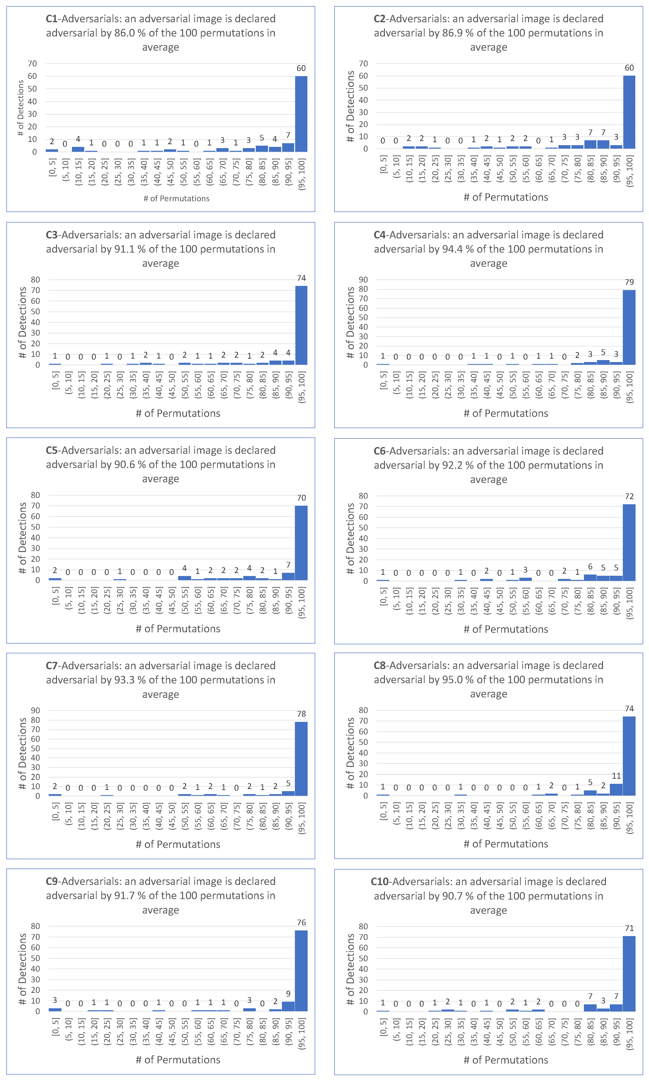
| EA-untargeted | 86.0 | 86.9 | 91.1 | 94.4 | 90.6 | 92.2 | 93.3 | 95.0 | 91.7 | 90.7 | 91.2 |
| 69.7 | 64.9 | 78.7 | 83.6 | 78.5 | 77.7 | 85.5 | 86.7 | 85.8 | 78.7 | 79.0 | |
| 100 | 100 | 98.9 | 100 | 100 | 100 | 100 | 100 | 98.9 | 98.9 | 99.6 | |
| 2 | 15 | 22 | 1 | 1 | 1 | 2 | 4 | 3 | 24 | 7.5 | |
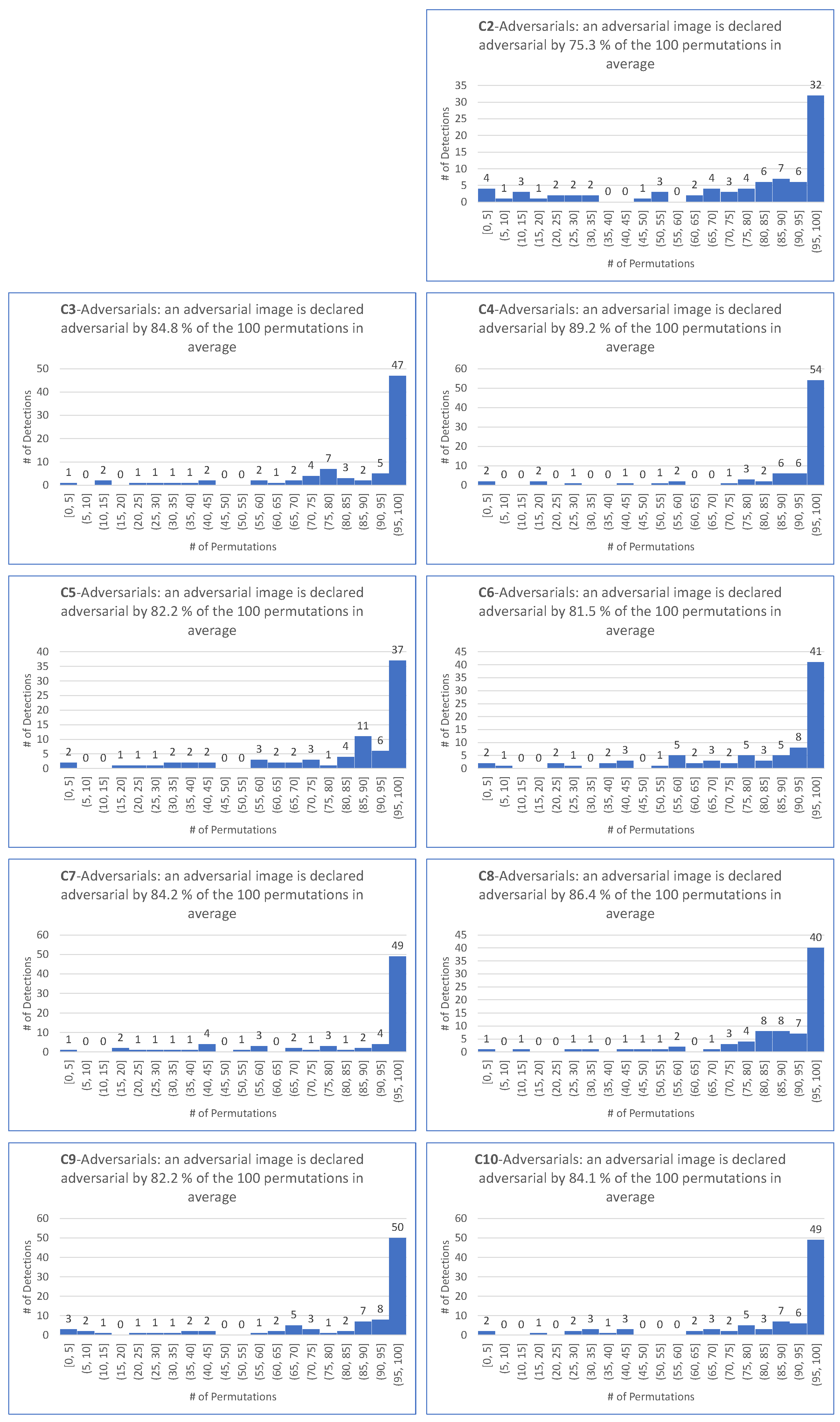
| FGSM-untargeted | NA | 75.3 | 84.8 | 89.2 | 82.2 | 81.5 | 84.2 | 86.4 | 82.2 | 84.1 | 83.3 |
| NA | 45.7 | 63.4 | 74.0 | 53.7 | 56.9 | 68.8 | 58.7 | 63.0 | 61.7 | 60.7 | |
| NA | 97.5 | 98.7 | 98.7 | 98.8 | 98.7 | 98.7 | 98.9 | 97.7 | 99.7 | 98.6 | |
| NA | 2 | 12 | 4 | 1 | 1 | 16 | 12 | 3 | 17 | 7.5 | |
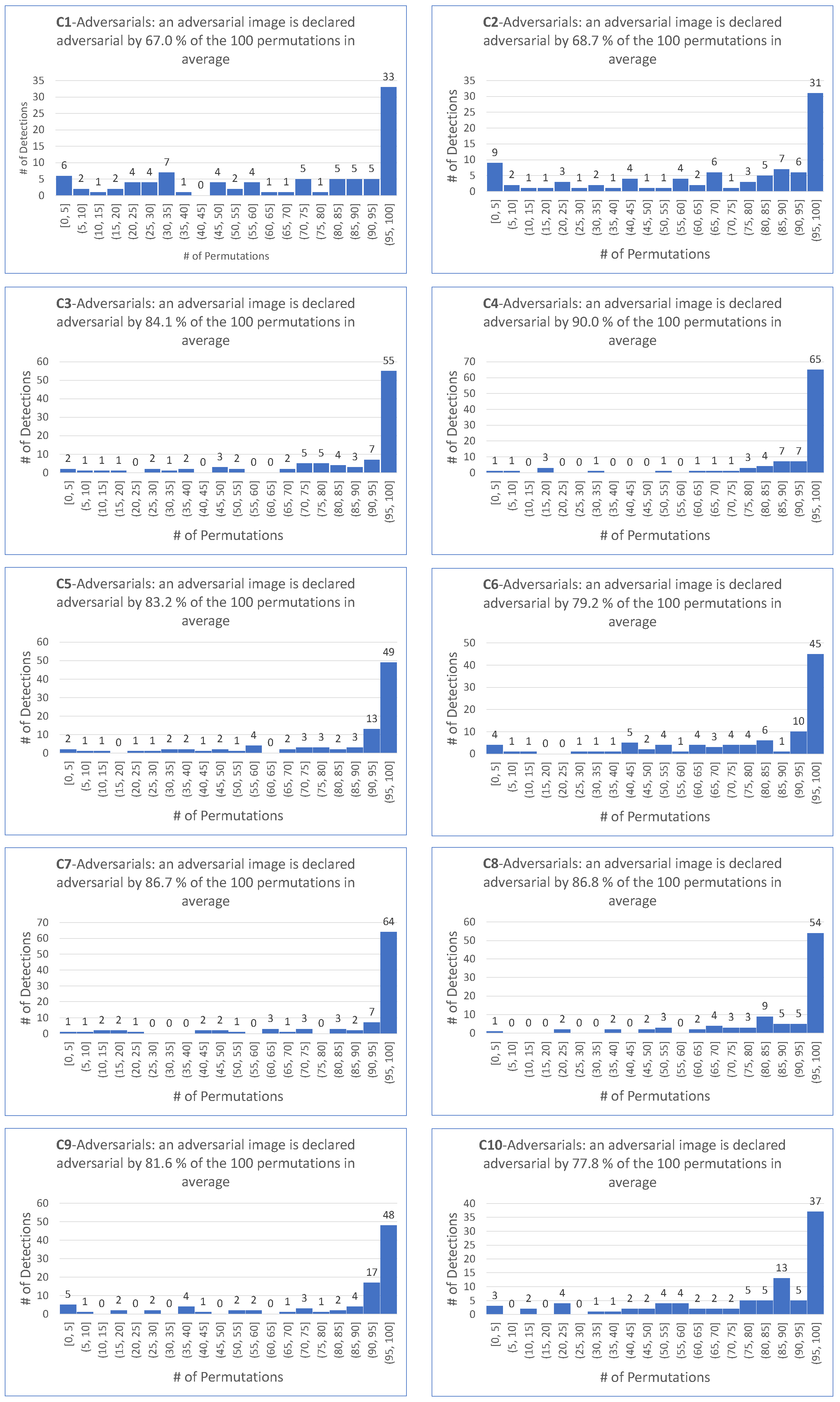
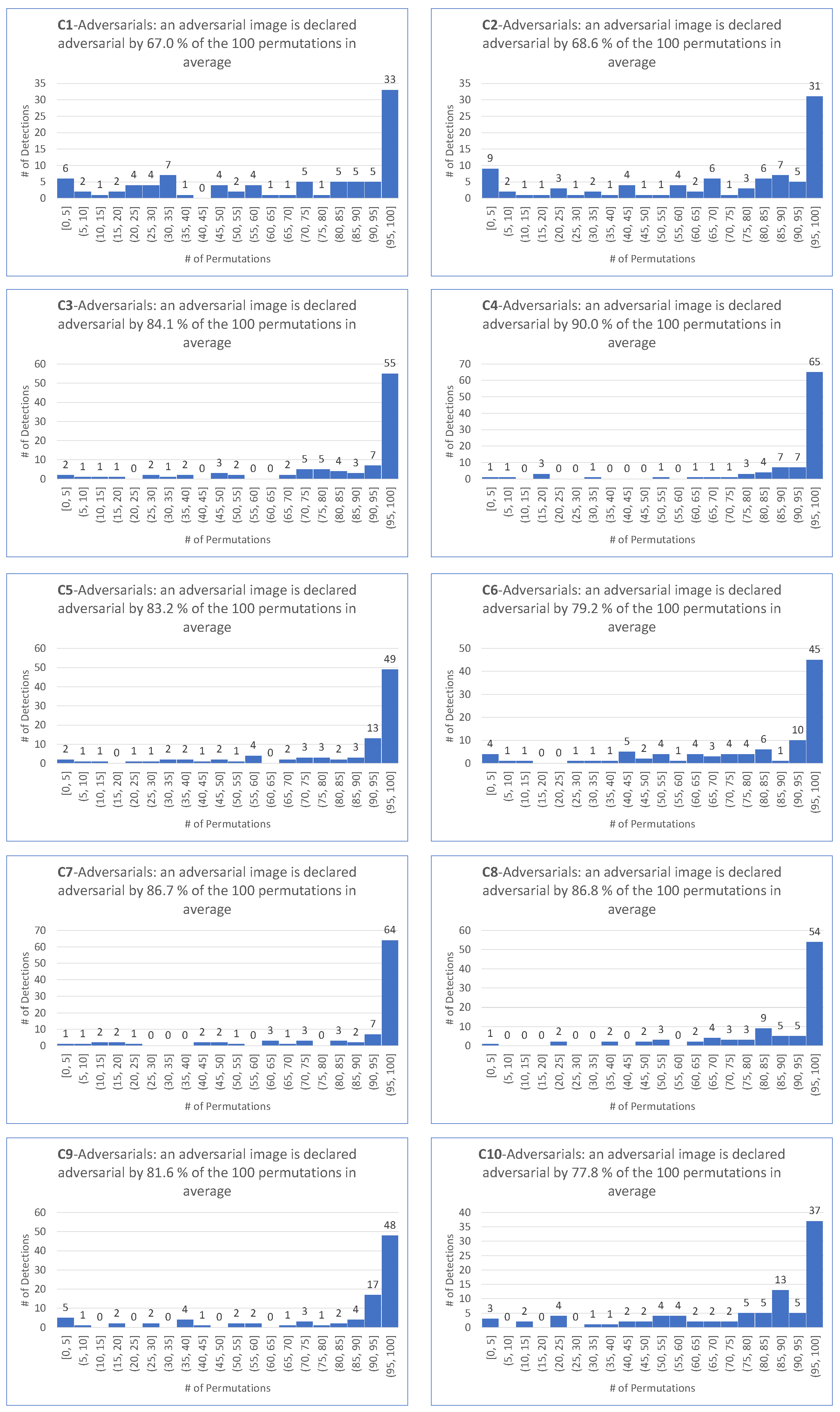
| BIM-untargeted | 67.0 | 68.7 | 84.1 | 90.1 | 83.2 | 79.2 | 86.7 | 86.8 | 81.6 | 77.8 | 80.6 |
| 40.8 | 40.6 | 64.5 | 75 | 66.6 | 56.1 | 74.7 | 62.1 | 68.4 | 44.6 | 59.3 | |
| 97.8 | 94.5 | 98.9 | 98.9 | 97.8 | 97.9 | 98.9 | 98.9 | 97.8 | 98.9 | 98.0 | |
| 1 | 1 | 3 | 9 | 9 | 3 | 10 | 21 | 1 | 2 | 6.0 | |
| PGD Inf-untargeted | 67.0 | 68.6 | 84.1 | 90.0 | 83.2 | 79.2 | 86.7 | 86.8 | 81.6 | 77.8 | 80.6 |
| 40.8 | 39.5 | 64.5 | 75 | 66.6 | 56.1 | 74.7 | 62.1 | 68.4 | 44.6 | 59.2 | |
| 97.8 | 94.5 | 98.9 | 98.9 | 97.8 | 97.9 | 98.9 | 98.9 | 97.8 | 98.9 | 98.0 | |
| 1 | 1 | 3 | 9 | 9 | 3 | 10 | 21 | 1 | 2 | 6.0 | |
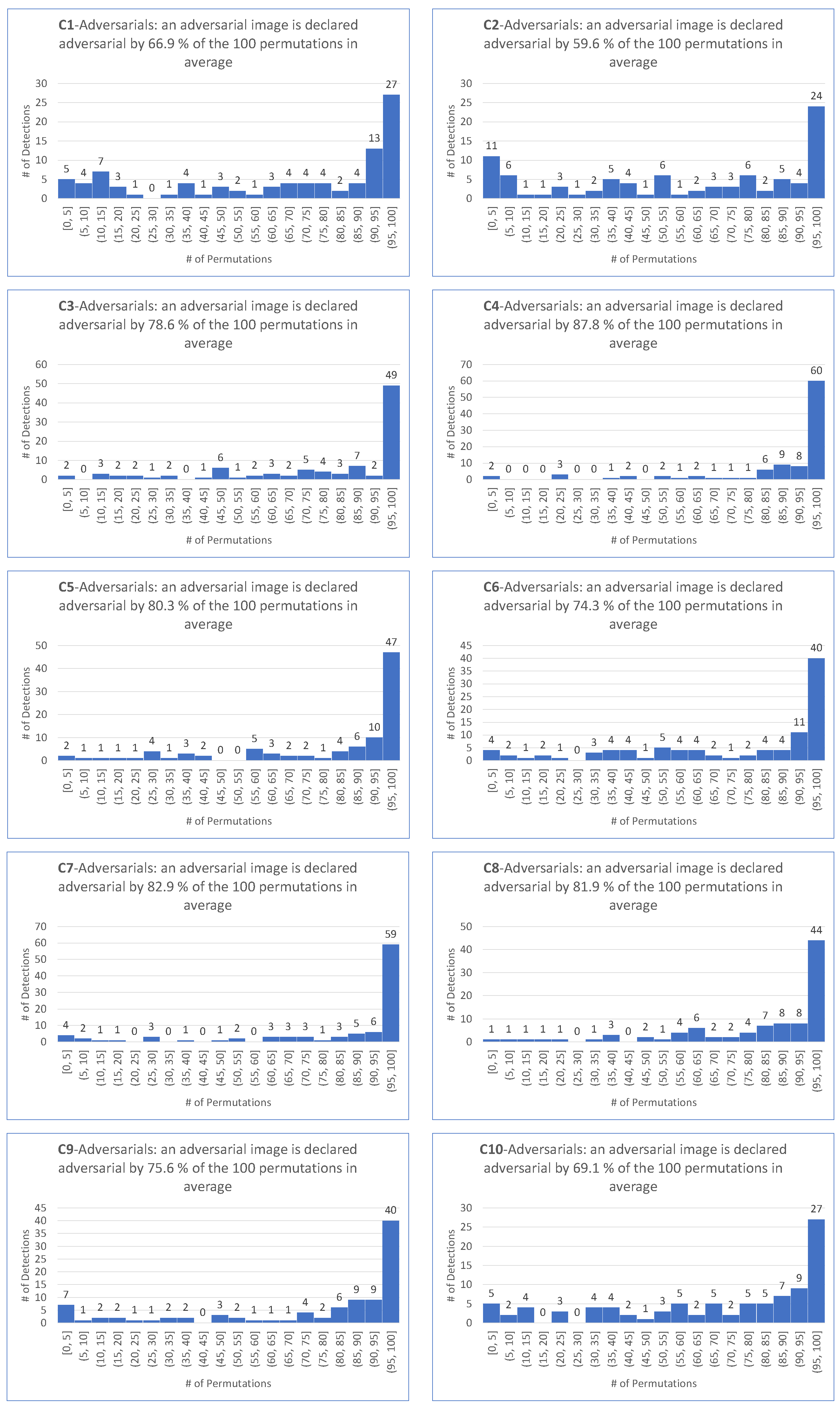
| PGD L2-untargeted | 66.9 | 59.6 | 78.6 | 87.8 | 80.3 | 74.3 | 82.9 | 81.9 | 75.6 | 69.1 | 75.9 |
| 43.0 | 30.7 | 52.5 | 68.6 | 59.3 | 51.5 | 66.3 | 53.6 | 51.0 | 37.8 | 51.4 | |
| 96.7 | 92.3 | 97.9 | 98.9 | 97.9 | 97.9 | 98.9 | 98.9 | 96.8 | 97.8 | 97.4 | |
| 1 | 1 | 13 | 1 | 8 | 2 | 3 | 8 | 1 | 3 | 4.1 | |
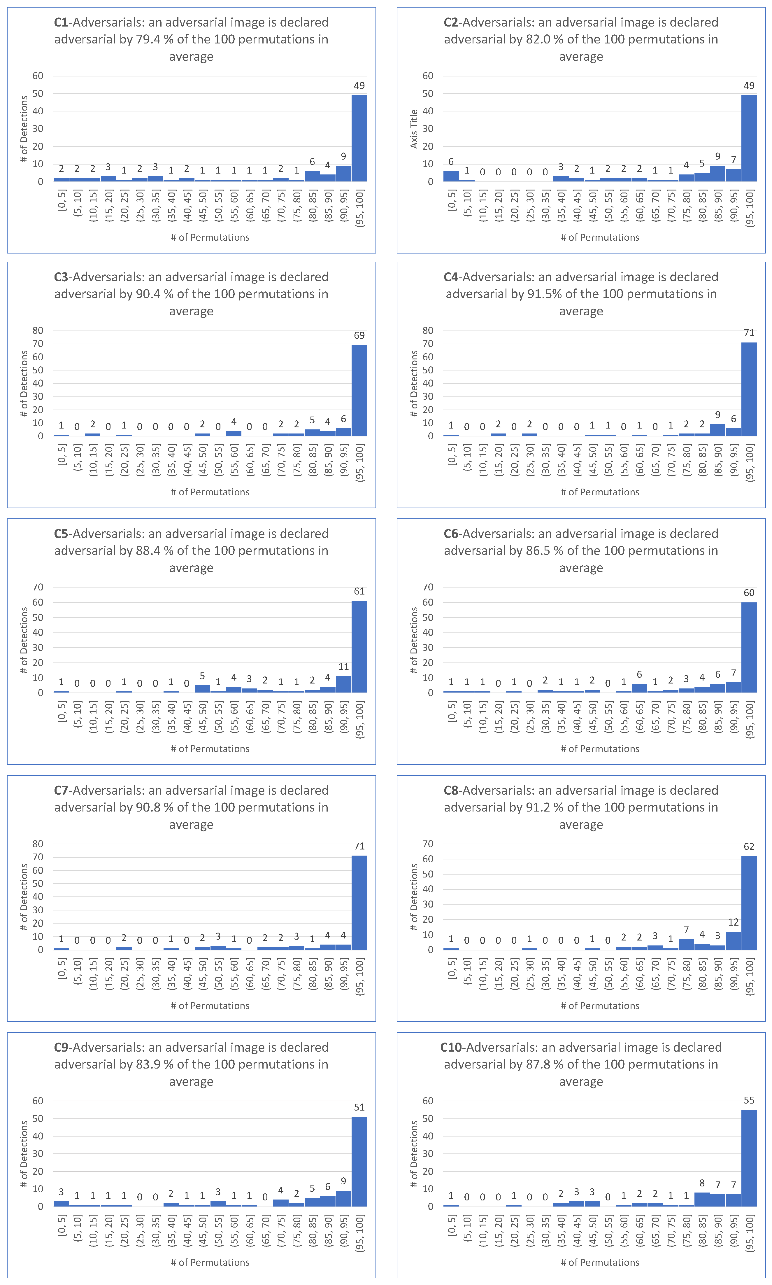
| CW Inf-untargeted | 79.4 | 82.0 | 90.4 | 91.5 | 88.4 | 86.5 | 90.8 | 91.2 | 83.9 | 87.8 | 87.3 |
| 61.7 | 58.9 | 76.5 | 77.7 | 73.4 | 67.0 | 77.3 | 74.7 | 64.5 | 65.9 | 69.7 | |
| 97.8 | 98.9 | 98.9 | 98.9 | 98.9 | 99 | 98.9 | 98.9 | 97.8 | 98.9 | 98.7 | |
| 7 | 1 | 15 | 18 | 24 | 10 | 24 | 27 | 1 | 25 | 15.2 | |
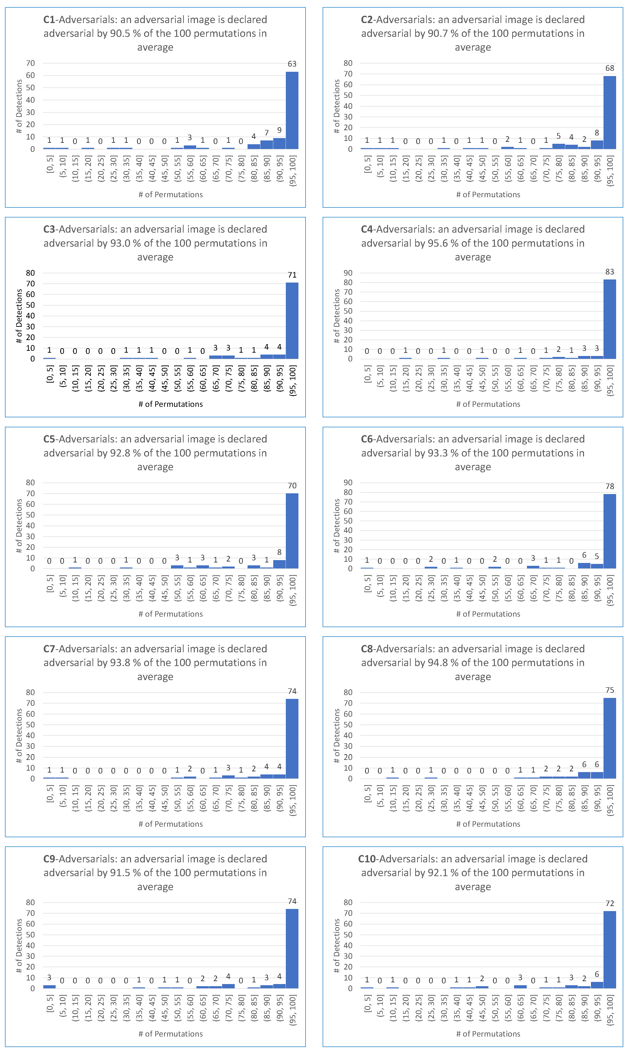
| DeepFool-untargeted | 90.5 | 90.7 | 93.0 | 95.6 | 92.8 | 93.3 | 93.8 | 94.8 | 91.5 | 92.1 | 92.8 |
| 76.5 | 78.3 | 81.5 | 88.6 | 82.9 | 83 | 82.9 | 83.5 | 81.2 | 82.9 | 82.1 | |
| 100 | 100 | 98.9 | 100 | 100 | 99 | 100 | 100 | 98.9 | 98.9 | 99.5 | |
| 1 | 2 | 35 | 16 | 12 | 28 | 5 | 12 | 1 | 12 | 12.4 |
| 51 | 38 | 38 | 30 | 34 | 33 | 26 | 25 | 26 | 40 | 37 | 32.7 |
| 54 | 37 | 36 | 29 | 33 | 30 | 25 | 23 | 25 | 40 | 36 | 31.4 |
| 87 | 24 | 13 | 16 | 19 | 14 | 15 | 13 | 12 | 29 | 19 | 17.4 |
| 91 | 23 | 13 | 14 | 18 | 12 | 13 | 11 | 8 | 23 | 15 | 15 |
| Targeted Attack | Metrics | Avg | |||||||||||
|---|---|---|---|---|---|---|---|---|---|---|---|---|---|
| 0.51 | EA | DR | 100 | 100 | 100 | 100 | 100 | 100 | 100 | 100 | 100 | 100 | 100 |
| TP | 91 | 90 | 88 | 84 | 79 | 85 | 89 | 86 | 97 | 97 | 88.6 | ||
| FP | 37 | 37 | 28 | 32 | 29 | 25 | 23 | 25 | 39 | 37 | 31.2 | ||
| FN | 0 | 0 | 0 | 0 | 0 | 0 | 0 | 0 | 0 | 0 | 0 | ||
| Precision | 0.71 | 0.70 | 0.75 | 0.72 | 0.73 | 0.77 | 0.79 | 0.77 | 0.71 | 0.72 | 0.73 | ||
| Recall | 1 | 1 | 1 | 1 | 1 | 1 | 1 | 1 | 1 | 1 | 1 | ||
| F1 | 0.83 | 0.82 | 0.85 | 0.83 | 0.84 | 0.87 | 0.88 | 0.87 | 0.83 | 0.83 | 0.84 | ||
| BIM | DR | 100 | 100 | 100 | 100 | 100 | 100 | 100 | 100 | 100 | 100 | 100 | |
| TP | 43 | 38 | 57 | 52 | 46 | 56 | 73 | 50 | 87 | 78 | 58 | ||
| FP | 23 | 23 | 20 | 19 | 21 | 18 | 17 | 15 | 35 | 31 | 22.2 | ||
| FN | 0 | 0 | 0 | 0 | 0 | 0 | 0 | 0 | 0 | 0 | 0 | ||
| Precision | 0.65 | 0.62 | 0.74 | 0.73 | 0.68 | 0.75 | 0.81 | 0.76 | 0.71 | 0.71 | 0.71 | ||
| Recall | 1 | 1 | 1 | 1 | 1 | 1 | 1 | 1 | 1 | 1 | 1 | ||
| F1 | 0.78 | 0.76 | 0.85 | 0.84 | 0.8 | 0.85 | 0.89 | 0.86 | 0.83 | 0.83 | 0.82 | ||
| PGD Inf | DR | 100 | 100 | 100 | 100 | 100 | 100 | 100 | 100 | 100 | 100 | 100 | |
| TP | 49 | 38 | 57 | 52 | 46 | 56 | 73 | 50 | 87 | 78 | 58.6 | ||
| FP | 23 | 23 | 20 | 19 | 21 | 18 | 17 | 15 | 35 | 31 | 22.2 | ||
| FN | 0 | 0 | 0 | 0 | 0 | 0 | 0 | 0 | 0 | 0 | 0 | ||
| Precision | 0.68 | 0.62 | 0.74 | 0.73 | 0.68 | 0.75 | 0.81 | 0.76 | 0.71 | 0.71 | 0.71 | ||
| Recall | 1 | 1 | 1 | 1 | 1 | 1 | 1 | 1 | 1 | 1 | 1 | ||
| F1 | 0.80 | 0.76 | 0.85 | 0.84 | 0.80 | 0.85 | 0.89 | 0.86 | 0.83 | 0.83 | 0.83 | ||
| PGD L2 | DR | 100 | 100 | 100 | 100 | 100 | 100 | 100 | 100 | 100 | 100 | 100 | |
| TP | 90 | 88 | 94 | 92 | 89 | 94 | 94 | 86 | 97 | 99 | 92.3 | ||
| FP | 23 | 23 | 20 | 31 | 29 | 26 | 24 | 24 | 38 | 36 | 27.4 | ||
| FN | 0 | 0 | 0 | 0 | 0 | 0 | 0 | 0 | 0 | 0 | 0 | ||
| Precision | 0.79 | 0.79 | 0.82 | 0.74 | 0.75 | 0.78 | 0.79 | 0.78 | 0.71 | 0.73 | 0.76 | ||
| Recall | 1 | 1 | 1 | 1 | 1 | 1 | 1 | 1 | 1 | 1 | 1 | ||
| F1 | 0.88 | 0.88 | 0.90 | 0.85 | 0.85 | 0.87 | 0.88 | 0.87 | 0.83 | 0.84 | 0.86 | ||
| 0.54 | EA | DR | 100 | 100 | 100 | 100 | 100 | 100 | 100 | 100 | 100 | 100 | 100 |
| TP | 91 | 90 | 88 | 84 | 79 | 85 | 89 | 86 | 97 | 97 | 88.6 | ||
| FP | 36 | 35 | 27 | 31 | 26 | 24 | 21 | 24 | 39 | 36 | 29.9 | ||
| FN | 0 | 0 | 0 | 0 | 0 | 0 | 0 | 0 | 0 | 0 | 0 | ||
| Precision | 0.71 | 0.72 | 0.76 | 0.73 | 0.75 | 0.77 | 0.80 | 0.78 | 0.71 | 0.72 | 0.74 | ||
| Recall | 1 | 1 | 1 | 1 | 1 | 1 | 1 | 1 | 1 | 1 | 1 | ||
| F1 | 0.83 | 0.83 | 0.86 | 0.84 | 0.85 | 0.87 | 0.88 | 0.87 | 0.83 | 0.83 | 0.84 | ||
| BIM | DR | 100 | 100 | 100 | 100 | 100 | 100 | 100 | 100 | 100 | 100 | 100 | |
| TP | 43 | 38 | 57 | 52 | 46 | 56 | 73 | 50 | 87 | 78 | 58 | ||
| FP | 22 | 22 | 19 | 19 | 19 | 18 | 16 | 14 | 35 | 30 | 21.4 | ||
| FN | 0 | 0 | 0 | 0 | 0 | 0 | 0 | 0 | 0 | 0 | 0 | ||
| Precision | 0.66 | 0.63 | 0.75 | 0.73 | 0.70 | 0.75 | 0.82 | 0.78 | 0.71 | 0.72 | 0.72 | ||
| Recall | 1 | 1 | 1 | 1 | 1 | 1 | 1 | 1 | 1 | 1 | 1 | ||
| F1 | 0.79 | 0.77 | 0.85 | 0.84 | 0.82 | 0.85 | 0.90 | 0.87 | 0.83 | 0.83 | 0.83 | ||
| PGD Inf | DR | 100 | 100 | 100 | 100 | 100 | 100 | 100 | 100 | 100 | 100 | 100 | |
| TP | 49 | 38 | 57 | 52 | 46 | 56 | 73 | 50 | 87 | 78 | 58.6 | ||
| FP | 22 | 22 | 19 | 19 | 19 | 18 | 16 | 14 | 35 | 30 | 21.4 | ||
| FN | 0 | 0 | 0 | 0 | 0 | 0 | 0 | 0 | 0 | 0 | 0 | ||
| Precision | 0.69 | 0.63 | 0.75 | 0.73 | 0.70 | 0.75 | 0.82 | 0.78 | 0.71 | 0.72 | 0.72 | ||
| Recall | 1 | 1 | 1 | 1 | 1 | 1 | 1 | 1 | 1 | 1 | 1 | ||
| F1 | 0.81 | 0.77 | 0.85 | 0.84 | 0.82 | 0.85 | 0.9 | 0.87 | 0.83 | 0.83 | 0.83 | ||
| PGD L2 | DR | 100 | 100 | 100 | 100 | 100 | 100 | 100 | 100 | 100 | 100 | 100 | |
| TP | 90 | 88 | 94 | 92 | 89 | 94 | 94 | 86 | 97 | 99 | 92.3 | ||
| FP | 22 | 22 | 19 | 30 | 26 | 25 | 22 | 23 | 38 | 35 | 26.2 | ||
| FN | 0 | 0 | 0 | 0 | 0 | 0 | 0 | 0 | 0 | 0 | 0 | ||
| Precision | 0.80 | 0.80 | 0.83 | 0.75 | 0.77 | 0.78 | 0.81 | 0.78 | 0.71 | 0.73 | 0.77 | ||
| Recall | 1 | 1 | 1 | 1 | 1 | 1 | 1 | 1 | 1 | 1 | 1 | ||
| F1 | 0.88 | 0.88 | 0.90 | 0.85 | 0.87 | 0.87 | 0.89 | 0.87 | 0.83 | 0.84 | 0.86 |
| Targeted Attack | Metrics | Avg | |||||||||||
|---|---|---|---|---|---|---|---|---|---|---|---|---|---|
| 0.87 | EA | DR | 100 | 100 | 100 | 100 | 100 | 100 | 100 | 100 | 100 | 100 | 100 |
| TP | 91 | 90 | 88 | 84 | 79 | 85 | 89 | 86 | 97 | 97 | 88.6 | ||
| FP | 23 | 13 | 16 | 18 | 12 | 15 | 12 | 12 | 29 | 19 | 16.9 | ||
| FN | 0 | 0 | 0 | 0 | 0 | 0 | 0 | 0 | 0 | 0 | 0 | ||
| Precision | 0.79 | 0.87 | 0.84 | 0.82 | 0.86 | 0.85 | 0.88 | 0.87 | 0.76 | 0.83 | 0.83 | ||
| Recall | 1 | 1 | 1 | 1 | 1 | 1 | 1 | 1 | 1 | 1 | 1 | ||
| F1 | 0.88 | 0.93 | 0.91 | 0.90 | 0.92 | 0.91 | 0.93 | 0.93 | 0.86 | 0.90 | 0.9 | ||
| BIM | DR | 100 | 100 | 100 | 98.1 | 97.8 | 98.2 | 98.6 | 100 | 100 | 98.7 | 99.1 | |
| TP | 43 | 38 | 57 | 51 | 45 | 55 | 72 | 50 | 87 | 77 | 57.5 | ||
| FP | 17 | 9 | 11 | 15 | 11 | 11 | 11 | 9 | 27 | 18 | 13.9 | ||
| FN | 0 | 0 | 0 | 1 | 1 | 1 | 1 | 0 | 0 | 1 | 0.5 | ||
| Precision | 0.71 | 0.80 | 0.83 | 0.77 | 0.80 | 0.83 | 0.86 | 0.84 | 0.76 | 0.81 | 0.8 | ||
| Recall | 1 | 1 | 1 | 0.98 | 0.978 | 0.982 | 0.986 | 1 | 1 | 0.987 | 0.99 | ||
| F1 | 0.83 | 0.88 | 0.90 | 0.86 | 0.88 | 0.89 | 0.91 | 0.91 | 0.86 | 0.88 | 0.87 | ||
| PGD Inf | DR | 100 | 100 | 100 | 98 | 97.8 | 98.2 | 98.6 | 100 | 100 | 98.7 | 99.1 | |
| TP | 49 | 38 | 57 | 51 | 45 | 55 | 72 | 50 | 87 | 77 | 58.1 | ||
| FP | 17 | 9 | 11 | 15 | 11 | 11 | 11 | 9 | 27 | 18 | 13.9 | ||
| FN | 0 | 0 | 0 | 1 | 1 | 1 | 1 | 0 | 0 | 1 | 0.5 | ||
| Precision | 0.74 | 0.80 | 0.83 | 0.77 | 0.80 | 0.83 | 0.86 | 0.84 | 0.76 | 0.81 | 0.8 | ||
| Recall | 1 | 1 | 1 | 0.98 | 0.978 | 0.982 | 0.986 | 1 | 1 | 0.987 | 0.99 | ||
| F1 | 0.85 | 0.88 | 0.90 | 0.86 | 0.88 | 0.89 | 0.91 | 0.91 | 0.86 | 0.88 | 0.88 | ||
| PGD L2 | DR | 100 | 100 | 100 | 98.9 | 98.8 | 98.9 | 98.9 | 100 | 100 | 98.9 | 99.4 | |
| TP | 90 | 88 | 94 | 91 | 88 | 93 | 93 | 86 | 97 | 98 | 91.8 | ||
| FP | 17 | 9 | 11 | 19 | 12 | 15 | 12 | 11 | 28 | 19 | 15.3 | ||
| FN | 0 | 0 | 0 | 1 | 1 | 1 | 1 | 0 | 0 | 1 | 0.5 | ||
| Precision | 0.84 | 0.90 | 0.89 | 0.82 | 0.88 | 0.86 | 0.88 | 0.88 | 0.77 | 0.83 | 0.85 | ||
| Recall | 1 | 1 | 1 | 0.98 | 0.98 | 0.98 | 0.98 | 1 | 1 | 0.98 | 0.99 | ||
| F1 | 0.91 | 0.94 | 0.94 | 0.89 | 0.92 | 0.91 | 0.92 | 0.93 | 0.87 | 0.89 | 0.91 | ||
| 0.91 | EA | DR | 100 | 100 | 100 | 100 | 100 | 100 | 100 | 100 | 100 | 100 | 100 |
| TP | 91 | 90 | 88 | 84 | 79 | 85 | 89 | 86 | 97 | 97 | 88.6 | ||
| FP | 23 | 13 | 14 | 17 | 11 | 13 | 10 | 8 | 23 | 15 | 14.7 | ||
| FN | 0 | 0 | 0 | 0 | 0 | 0 | 0 | 0 | 0 | 0 | 0 | ||
| Precision | 0.79 | 0.87 | 0.86 | 0.83 | 0.87 | 0.86 | 0.89 | 0.91 | 0.80 | 0.86 | 0.85 | ||
| Recall | 1 | 1 | 1 | 1 | 1 | 1 | 1 | 1 | 1 | 1 | 1 | ||
| F1 | 0.88 | 0.93 | 0.92 | 0.90 | 0.93 | 0.92 | 0.94 | 0.95 | 0.88 | 0.92 | 0.91 | ||
| BIM | DR | 100.00 | 100.00 | 100.00 | 98.00 | 97.80 | 98.20 | 98.60 | 100.00 | 100.00 | 98.70 | 99.10 | |
| TP | 43 | 38 | 57 | 51 | 45 | 55 | 72 | 50 | 87 | 77 | 57.5 | ||
| FP | 17 | 9 | 9 | 15 | 10 | 9 | 9 | 7 | 22 | 14 | 12.1 | ||
| FN | 0 | 0 | 0 | 1 | 1 | 1 | 1 | 0 | 0 | 1 | 0.5 | ||
| Precision | 0.71 | 0.80 | 0.86 | 0.77 | 0.81 | 0.85 | 0.88 | 0.87 | 0.79 | 0.84 | 0.81 | ||
| Recall | 1 | 1 | 1 | 0.98 | 0.978 | 0.982 | 0.986 | 1 | 1 | 0.987 | 0.99 | ||
| F1 | 0.83 | 0.88 | 0.92 | 0.86 | 0.88 | 0.91 | 0.92 | 0.93 | 0.88 | 0.90 | 0.89 | ||
| PGD Inf | DR | 100 | 100 | 100 | 98 | 97.8 | 98.2 | 98.6 | 100 | 100 | 98.7 | 99.1 | |
| TP | 49 | 38 | 57 | 51 | 45 | 55 | 72 | 50 | 87 | 77 | 58.1 | ||
| FP | 17 | 9 | 9 | 15 | 10 | 9 | 9 | 7 | 22 | 14 | 12.1 | ||
| FN | 0 | 0 | 0 | 1 | 1 | 1 | 1 | 0 | 0 | 1 | 0.5 | ||
| Precision | 0.74 | 0.80 | 0.86 | 0.77 | 0.81 | 0.85 | 0.88 | 0.87 | 0.79 | 0.84 | 0.82 | ||
| Recall | 1 | 1 | 1 | 0.98 | 0.97 | 0.98 | 0.98 | 1 | 1 | 0.98 | 0.99 | ||
| F1 | 0.85 | 0.88 | 0.92 | 0.86 | 0.88 | 0.91 | 0.92 | 0.93 | 0.88 | 0.90 | 0.89 | ||
| PGD L2 | DR | 100 | 100 | 100 | 98.9 | 98.8 | 97.8 | 98.9 | 98.8 | 100 | 97.9 | 99.1 | |
| TP | 90 | 88 | 94 | 91 | 88 | 92 | 93 | 85 | 97 | 97 | 91.5 | ||
| FP | 17 | 9 | 9 | 18 | 11 | 13 | 10 | 8 | 22 | 15 | 13.2 | ||
| FN | 0 | 0 | 0 | 1 | 1 | 2 | 1 | 1 | 0 | 2 | 0.8 | ||
| Precision | 0.84 | 0.90 | 0.91 | 0.83 | 0.88 | 0.87 | 0.90 | 0.91 | 0.81 | 0.86 | 0.87 | ||
| Recall | 1 | 1 | 1 | 0.989 | 0.988 | 0.978 | 0.989 | 0.988 | 1 | 0.979 | 0.99 | ||
| F1 | 0.91 | 0.94 | 0.95 | 0.9 | 0.93 | 0.92 | 0.94 | 0.94 | 0.89 | 0.91 | 0.91 |
| Untargeted Attack | Metrics | Avg | |||||||||||
|---|---|---|---|---|---|---|---|---|---|---|---|---|---|
| 0.51 | EA | DR | 88.5 | 90.7 | 93.9 | 96.9 | 96.9 | 95.9 | 96.9 | 97.9 | 93.9 | 93.9 | 94.5 |
| TP | 85 | 88 | 93 | 95 | 95 | 95 | 94 | 96 | 93 | 93 | 92.7 | ||
| FP | 38 | 38 | 29 | 34 | 33 | 26 | 25 | 26 | 39 | 36 | 32.4 | ||
| FN | 11 | 9 | 6 | 3 | 3 | 4 | 3 | 2 | 6 | 6 | 5.3 | ||
| Precision | 0.69 | 0.69 | 0.76 | 0.73 | 0.74 | 0.78 | 0.78 | 0.78 | 0.70 | 0.72 | 0.74 | ||
| Recall | 0.88 | 0.90 | 0.93 | 0.96 | 0.96 | 0.95 | 0.96 | 0.97 | 0.93 | 0.93 | 0.94 | ||
| F1 | 0.77 | 0.78 | 0.83 | 0.82 | 0.83 | 0.85 | 0.86 | 0.86 | 0.79 | 0.81 | 0.82 | ||
| FGSM | DR | 80.7 | 89.0 | 92.5 | 86.2 | 87.2 | 85.7 | 92.5 | 85.8 | 86.5 | 87.3 | ||
| TP | 67 | 73 | 75 | 69 | 75 | 66 | 74 | 79 | 77 | 72.7 | |||
| FP | 33 | 28 | 31 | 29 | 23 | 22 | 23 | 34 | 30 | 28.1 | |||
| FN | 16 | 9 | 6 | 11 | 11 | 11 | 6 | 13 | 12 | 10.5 | |||
| Precision | 0.67 | 0.72 | 0.70 | 0.70 | 0.76 | 0.75 | 0.76 | 0.69 | 0.71 | 0.72 | |||
| Recall | 0.80 | 0.89 | 0.92 | 0.86 | 0.87 | 0.85 | 0.92 | 0.85 | 0.86 | 0.87 | |||
| F1 | 0.72 | 0.79 | 0.79 | 0.77 | 0.81 | 0.79 | 0.83 | 0.76 | 0.77 | 0.78 | |||
| BIM | DR | 66.6 | 72.5 | 86.4 | 93.7 | 86.0 | 83.6 | 88.4 | 92.6 | 84.2 | 84.0 | 83.8 | |
| TP | 62 | 66 | 83 | 90 | 80 | 82 | 84 | 88 | 80 | 79 | 79.4 | ||
| FP | 34 | 32 | 28 | 32 | 29 | 24 | 22 | 24 | 33 | 31 | 28.9 | ||
| FN | 31 | 25 | 13 | 6 | 13 | 16 | 11 | 7 | 15 | 15 | 15.2 | ||
| Precision | 0.64 | 0.67 | 0.74 | 0.73 | 0.73 | 0.77 | 0.79 | 0.78 | 0.70 | 0.71 | 0.73 | ||
| Recall | 0.66 | 0.72 | 0.86 | 0.93 | 0.86 | 0.83 | 0.88 | 0.92 | 0.84 | 0.84 | 0.83 | ||
| F1 | 0.64 | 0.69 | 0.79 | 0.81 | 0.78 | 0.79 | 0.83 | 0.84 | 0.76 | 0.76 | 0.77 | ||
| PGD Inf | DR | 66.6 | 72.5 | 86.4 | 93.7 | 86.0 | 83.6 | 88.4 | 92.6 | 84.2 | 84.0 | 83.8 | |
| TP | 62 | 66 | 83 | 90 | 80 | 82 | 84 | 88 | 80 | 79 | 79.4 | ||
| FP | 34 | 32 | 28 | 32 | 29 | 24 | 22 | 24 | 33 | 31 | 28.9 | ||
| FN | 31 | 25 | 13 | 6 | 13 | 16 | 11 | 7 | 15 | 15 | 15.2 | ||
| Precision | 0.64 | 0.67 | 0.74 | 0.73 | 0.73 | 0.77 | 0.79 | 0.78 | 0.70 | 0.71 | 0.73 | ||
| Recall | 0.66 | 0.72 | 0.86 | 0.93 | 0.86 | 0.83 | 0.88 | 0.92 | 0.84 | 0.84 | 0.83 | ||
| F1 | 0.64 | 0.69 | 0.79 | 0.81 | 0.78 | 0.79 | 0.83 | 0.84 | 0.76 | 0.76 | 0.77 | ||
| PGD L2 | DR | 68.8 | 61.5 | 80.4 | 91.9 | 83.3 | 77.7 | 86.7 | 88.6 | 78.1 | 73.6 | 79.0 | |
| TP | 64 | 56 | 78 | 91 | 80 | 77 | 85 | 86 | 75 | 70 | 76.2 | ||
| FP | 34 | 31 | 27 | 32 | 29 | 24 | 22 | 24 | 34 | 32 | 28.9 | ||
| FN | 29 | 35 | 19 | 8 | 16 | 22 | 13 | 11 | 21 | 25 | 19.9 | ||
| Precision | 0.65 | 0.64 | 0.74 | 0.73 | 0.73 | 0.76 | 0.79 | 0.78 | 0.68 | 0.68 | 0.72 | ||
| Recall | 0.68 | 0.61 | 0.80 | 0.91 | 0.83 | 0.77 | 0.86 | 0.88 | 0.78 | 0.73 | 0.79 | ||
| F1 | 0.66 | 0.62 | 0.76 | 0.81 | 0.77 | 0.76 | 0.82 | 0.82 | 0.72 | 0.7 | 0.75 | ||
| CW Inf | DR | 79.7 | 86.3 | 93.8 | 93.9 | 91.8 | 90.0 | 93.8 | 96.9 | 88.1 | 89.3 | 90.3 | |
| TP | 75 | 82 | 92 | 93 | 90 | 90 | 91 | 96 | 82 | 84 | 87.5 | ||
| FP | 34 | 33 | 28 | 32 | 30 | 25 | 21 | 24 | 31 | 30 | 28.8 | ||
| FN | 19 | 13 | 6 | 6 | 8 | 10 | 6 | 3 | 11 | 10 | 9.2 | ||
| Precision | 0.68 | 0.71 | 0.76 | 0.74 | 0.75 | 0.78 | 0.81 | 0.80 | 0.72 | 0.73 | 0.75 | ||
| Recall | 0.79 | 0.86 | 0.93 | 0.93 | 0.91 | 0.90 | 0.93 | 0.96 | 0.88 | 0.89 | 0.90 | ||
| F1 | 0.73 | 0.77 | 0.83 | 0.82 | 0.82 | 0.83 | 0.86 | 0.87 | 0.79 | 0.8 | 0.81 | ||
| DeepFool | DR | 94.6 | 93.8 | 95.6 | 96.9 | 97.8 | 96.0 | 97.8 | 97.9 | 94.7 | 93.6 | 95.8 | |
| TP | 89 | 91 | 88 | 94 | 92 | 96 | 92 | 95 | 91 | 88 | 91.6 | ||
| FP | 36 | 37 | 27 | 33 | 28 | 25 | 22 | 25 | 37 | 32 | 30.2 | ||
| FN | 5 | 6 | 4 | 3 | 2 | 4 | 2 | 2 | 5 | 6 | 3.9 | ||
| Precision | 0.71 | 0.71 | 0.76 | 0.74 | 0.76 | 0.79 | 0.80 | 0.79 | 0.71 | 0.73 | 0.75 | ||
| Recall | 0.94 | 0.93 | 0.95 | 0.96 | 0.97 | 0.96 | 0.97 | 0.97 | 0.94 | 0.93 | 0.95 | ||
| F1 | 0.8 | 0.8 | 0.84 | 0.83 | 0.85 | 0.86 | 0.87 | 0.87 | 0.8 | 0.81 | 0.83 |
| Untargeted Attack | Metrics | Avg | |||||||||||
|---|---|---|---|---|---|---|---|---|---|---|---|---|---|
| 0.91 | EA | DR | 69.7 | 64.9 | 78.7 | 83.6 | 78.5 | 77.7 | 85.5 | 86.7 | 85.8 | 78.7 | 78.9 |
| TP | 67 | 63 | 78 | 82 | 77 | 77 | 83 | 85 | 85 | 78 | 77.5 | ||
| FP | 23 | 13 | 13 | 18 | 12 | 13 | 11 | 8 | 22 | 14 | 14.7 | ||
| FN | 29 | 34 | 21 | 16 | 21 | 22 | 14 | 13 | 14 | 21 | 20.5 | ||
| Precision | 0.74 | 0.82 | 0.85 | 0.82 | 0.86 | 0.85 | 0.88 | 0.91 | 0.79 | 0.84 | 0.83 | ||
| Recall | 0.69 | 0.64 | 0.78 | 0.83 | 0.78 | 0.77 | 0.85 | 0.86 | 0.85 | 0.78 | 0.78 | ||
| F1 | 0.71 | 0.71 | 0.81 | 0.82 | 0.81 | 0.8 | 0.86 | 0.88 | 0.81 | 0.8 | 0.8 | ||
| FGSM | DR | 45.7 | 63.4 | 74.0 | 53.7 | 56.9 | 68.8 | 58.7 | 63.0 | 61.7 | 60.7 | ||
| TP | 38 | 52 | 60 | 43 | 49 | 53 | 47 | 58 | 55 | 50.6 | |||
| FP | 11 | 13 | 16 | 9 | 12 | 10 | 8 | 17 | 11 | 11.9 | |||
| FN | 45 | 30 | 21 | 37 | 37 | 24 | 33 | 34 | 34 | 32.8 | |||
| Precision | 0.77 | 0.80 | 0.78 | 0.82 | 0.80 | 0.84 | 0.85 | 0.77 | 0.83 | 0.8 | |||
| Recall | 0.45 | 0.63 | 0.74 | 0.53 | 0.56 | 0.68 | 0.58 | 0.63 | 0.61 | 0.6 | |||
| F1 | 0.56 | 0.7 | 0.75 | 0.64 | 0.65 | 0.75 | 0.68 | 0.69 | 0.7 | 0.68 | |||
| BIM | DR | 40.8 | 40.6 | 64.5 | 75.0 | 66.6 | 56.1 | 74.7 | 62.1 | 68.4 | 44.6 | 59.3 | |
| TP | 38 | 37 | 62 | 72 | 62 | 55 | 71 | 59 | 65 | 42 | 56.3 | ||
| FP | 20 | 11 | 13 | 16 | 9 | 12 | 10 | 8 | 16 | 11 | 12.6 | ||
| FN | 55 | 54 | 34 | 24 | 31 | 43 | 25 | 36 | 30 | 52 | 38.4 | ||
| Precision | 0.65 | 0.77 | 0.82 | 0.81 | 0.87 | 0.82 | 0.87 | 0.88 | 0.80 | 0.79 | 0.8 | ||
| Recall | 0.40 | 0.40 | 0.64 | 0.75 | 0.66 | 0.56 | 0.73 | 0.62 | 0.68 | 0.44 | 0.58 | ||
| F1 | 0.49 | 0.52 | 0.71 | 0.77 | 0.75 | 0.66 | 0.79 | 0.72 | 0.73 | 0.56 | 0.67 | ||
| PGD Inf | DR | 40.8 | 39.5 | 64.5 | 75.0 | 66.6 | 56.1 | 74.7 | 62.1 | 68.4 | 44.6 | 59.2 | |
| TP | 38 | 36 | 62 | 72 | 62 | 55 | 71 | 59 | 65 | 42 | 56.2 | ||
| FP | 20 | 13 | 13 | 16 | 9 | 12 | 10 | 8 | 16 | 11 | 12.8 | ||
| FN | 55 | 55 | 34 | 24 | 31 | 43 | 24 | 36 | 30 | 52 | 38.4 | ||
| Precision | 0.65 | 0.73 | 0.82 | 0.81 | 0.87 | 0.82 | 0.87 | 0.88 | 0.80 | 0.79 | 0.8 | ||
| Recall | 0.40 | 0.39 | 0.64 | 0.75 | 0.66 | 0.56 | 0.74 | 0.62 | 0.68 | 0.44 | 0.58 | ||
| F1 | 0.49 | 0.5 | 0.71 | 0.77 | 0.75 | 0.66 | 0.79 | 0.72 | 0.73 | 0.56 | 0.66 | ||
| PGD L2 | DR | 43.0 | 30.7 | 52.5 | 68.6 | 59.3 | 51.5 | 66.3 | 53.6 | 51.0 | 37.8 | 51.4 | |
| TP | 40 | 28 | 51 | 68 | 57 | 51 | 65 | 52 | 49 | 36 | 49.7 | ||
| FP | 20 | 11 | 12 | 16 | 9 | 12 | 10 | 8 | 17 | 12 | 12.7 | ||
| FN | 53 | 63 | 46 | 31 | 39 | 48 | 33 | 45 | 47 | 59 | 46.4 | ||
| Precision | 0.66 | 0.71 | 0.80 | 0.80 | 0.86 | 0.80 | 0.86 | 0.86 | 0.74 | 0.75 | 0.78 | ||
| Recall | 0.43 | 0.30 | 0.52 | 0.68 | 0.59 | 0.51 | 0.66 | 0.53 | 0.51 | 0.37 | 0.51 | ||
| F1 | 0.52 | 0.42 | 0.63 | 0.73 | 0.69 | 0.62 | 0.74 | 0.65 | 0.6 | 0.49 | 0.6 | ||
| CW Inf | DR | 61.7 | 58.9 | 76.5 | 77.7 | 73.4 | 67.0 | 77.3 | 74.7 | 64.5 | 65.9 | 69.7 | |
| TP | 58 | 56 | 75 | 77 | 72 | 67 | 75 | 74 | 60 | 62 | 67.6 | ||
| FP | 20 | 11 | 13 | 16 | 10 | 12 | 9 | 8 | 14 | 11 | 12.4 | ||
| FN | 36 | 39 | 23 | 22 | 26 | 33 | 22 | 25 | 33 | 32 | 29.1 | ||
| Precision | 0.74 | 0.83 | 0.85 | 0.82 | 0.87 | 0.84 | 0.89 | 0.90 | 0.81 | 0.84 | 0.83 | ||
| Recall | 0.61 | 0.58 | 0.76 | 0.77 | 0.73 | 0.67 | 0.77 | 0.74 | 0.64 | 0.65 | 0.69 | ||
| F1 | 0.66 | 0.68 | 0.8 | 0.79 | 0.79 | 0.74 | 0.82 | 0.81 | 0.71 | 0.73 | 0.75 | ||
| DeepFool | DR | 76.5 | 78.3 | 81.5 | 88.6 | 82.9 | 83.0 | 82.9 | 83.5 | 81.2 | 82.9 | 82.1 | |
| TP | 72 | 76 | 75 | 86 | 78 | 83 | 78 | 81 | 78 | 78 | 78.5 | ||
| FP | 22 | 12 | 12 | 17 | 12 | 12 | 9 | 8 | 20 | 12 | 13.6 | ||
| FN | 22 | 21 | 17 | 11 | 16 | 17 | 16 | 16 | 18 | 16 | 17 | ||
| Precision | 0.76 | 0.86 | 0.86 | 0.83 | 0.86 | 0.87 | 0.89 | 0.91 | 0.79 | 0.86 | 0.84 | ||
| Recall | 0.76 | 0.78 | 0.81 | 0.88 | 0.82 | 0.83 | 0.82 | 0.83 | 0.81 | 0.82 | 0.81 | ||
| F1 | 0.76 | 0.81 | 0.83 | 0.85 | 0.83 | 0.84 | 0.85 | 0.86 | 0.79 | 0.83 | 0.82 |
| Targeted Attacks | ||||||||||||
|---|---|---|---|---|---|---|---|---|---|---|---|---|
| Avg | ||||||||||||
| 0.51 | DR | 100 | 100 | 100 | 100 | 100 | 100 | 100 | 100 | 100 | 100 | 100 |
| TP | 68.3 | 63.5 | 74.0 | 70.0 | 65.0 | 72.8 | 82.3 | 68.0 | 92.0 | 88.0 | 74.4 | |
| FP | 26.5 | 26.5 | 22.0 | 25.3 | 25.0 | 21.8 | 20.3 | 19.8 | 36.8 | 33.8 | 25.8 | |
| FN | 0 | 0 | 0 | 0 | 0 | 0 | 0 | 0 | 0 | 0 | 0 | |
| Precision | 0.71 | 0.68 | 0.76 | 0.73 | 0.71 | 0.76 | 0.80 | 0.77 | 0.71 | 0.72 | 0.73 | |
| Recall | 1 | 1 | 1 | 1 | 1 | 1 | 1 | 1 | 1 | 1 | 1 | |
| F1 | 0.82 | 0.81 | 0.86 | 0.84 | 0.82 | 0.86 | 0.89 | 0.87 | 0.83 | 0.83 | 0.84 | |
| F1 | 0.78 | 0.76 | 0.85 | 0.83 | 0.80 | 0.85 | 0.88 | 0.86 | 0.83 | 0.83 | 0.82 | |
| 0.91 | DR | 100 | 100 | 100 | 98.73 | 98.6 | 98.55 | 99.03 | 99.7 | 100 | 98.83 | 99.34 |
| TP | 68.25 | 63.5 | 74 | 69.25 | 64.25 | 71.75 | 81.5 | 67.75 | 92 | 87 | 73.93 | |
| FP | 18.5 | 10 | 10.25 | 16.25 | 10.5 | 11 | 9.5 | 7.5 | 22.25 | 14.5 | 13.03 | |
| FN | 0 | 0 | 0 | 0.75 | 0.75 | 1 | 0.75 | 0.25 | 0 | 1 | 0.45 | |
| Precision | 0.77 | 0.84 | 0.87 | 0.8 | 0.84 | 0.86 | 0.89 | 0.89 | 0.79 | 0.85 | 0.84 | |
| Recall | 1 | 1 | 1 | 0.99 | 0.98 | 0.99 | 0.99 | 0.99 | 1 | 0.99 | 0.99 | |
| F1 | 0.87 | 0.91 | 0.93 | 0.88 | 0.91 | 0.92 | 0.93 | 0.94 | 0.88 | 0.91 | 0.90 | |
| F1 | 0.83 | 0.88 | 0.92 | 0.86 | 0.88 | 0.91 | 0.92 | 0.93 | 0.88 | 0.9 | 0.89 | |
| Untargeted Attacks | ||||||||||||
|---|---|---|---|---|---|---|---|---|---|---|---|---|
| Avg | ||||||||||||
| 0.51 | DR | 77.5 | 79.7 | 89.4 | 94.2 | 89.7 | 87.7 | 91.1 | 94.1 | 87.0 | 86.4 | 87.7 |
| TP | 72.8 | 73.7 | 84.3 | 89.7 | 83.7 | 85.3 | 85.1 | 89.0 | 82.9 | 81.4 | 82.8 | |
| FP | 35.0 | 33.7 | 27.9 | 32.3 | 29.6 | 24.4 | 22.3 | 24.3 | 34.4 | 31.7 | 29.6 | |
| FN | 21.0 | 18.4 | 10.0 | 5.4 | 9.4 | 11.9 | 8.1 | 5.4 | 12.3 | 12.7 | 11.5 | |
| Precision | 0.7 | 0.7 | 0.7 | 0.7 | 0.7 | 0.8 | 0.8 | 0.8 | 0.7 | 0.7 | 0.7 | |
| Recall | 0.8 | 0.8 | 0.9 | 0.9 | 0.9 | 0.9 | 0.9 | 0.9 | 0.9 | 0.9 | 0.9 | |
| F1 | 0.7 | 0.7 | 0.8 | 0.8 | 0.8 | 0.8 | 0.8 | 0.8 | 0.8 | 0.8 | 0.8 | |
| F1 | 0.64 | 0.62 | 0.76 | 0.81 | 0.77 | 0.76 | 0.82 | 0.82 | 0.72 | 0.70 | 0.7 | |
| 0.91 | DR | 55.42 | 51.23 | 68.8 | 77.5 | 68.71 | 64.04 | 75.74 | 68.77 | 68.9 | 59.46 | 65.86 |
| TP | 52.17 | 47.71 | 65 | 73.86 | 64.43 | 62.43 | 70.86 | 65.29 | 65.71 | 56.14 | 62.36 | |
| FP | 20.83 | 11.71 | 12.71 | 16.43 | 10 | 12.14 | 9.857 | 8 | 17.43 | 11.71 | 13.08 | |
| FN | 41.67 | 44.43 | 29.29 | 21.29 | 28.71 | 34.71 | 22.57 | 29.14 | 29.43 | 38 | 31.92 | |
| Precision | 0.70 | 0.78 | 0.83 | 0.81 | 0.86 | 0.83 | 0.87 | 0.88 | 0.79 | 0.81 | 0.82 | |
| Recall | 0.55 | 0.51 | 0.68 | 0.77 | 0.68 | 0.64 | 0.75 | 0.68 | 0.69 | 0.59 | 0.65 | |
| F1 | 0.61 | 0.60 | 0.74 | 0.78 | 0.75 | 0.71 | 0.80 | 0.76 | 0.72 | 0.67 | 0.71 | |
| F1 | 0.49 | 0.42 | 0.63 | 0.73 | 0.69 | 0.62 | 0.74 | 0.65 | 0.6 | 0.49 | 0.61 | |
| All Attacks | ||||||||||||
|---|---|---|---|---|---|---|---|---|---|---|---|---|
| Avg | ||||||||||||
| 0.51 | DR | 88.73 | 89.86 | 94.68 | 97.11 | 94.86 | 93.86 | 95.55 | 97.07 | 93.50 | 93.21 | 93.84 |
| TP | 70.54 | 68.61 | 79.14 | 79.86 | 74.36 | 79.02 | 83.70 | 78.50 | 87.43 | 84.71 | 78.59 | |
| FP | 30.75 | 30.11 | 24.93 | 28.77 | 27.29 | 23.09 | 21.27 | 22.02 | 35.59 | 32.73 | 27.65 | |
| FN | 10.50 | 9.21 | 5.00 | 2.71 | 4.71 | 5.93 | 4.07 | 2.71 | 6.14 | 6.36 | 5.74 | |
| Precision | 0.69 | 0.68 | 0.75 | 0.73 | 0.72 | 0.77 | 0.79 | 0.77 | 0.71 | 0.72 | 0.73 | |
| Recall | 0.88 | 0.90 | 0.94 | 0.97 | 0.95 | 0.94 | 0.95 | 0.97 | 0.93 | 0.93 | 0.94 | |
| F1 | 0.76 | 0.76 | 0.83 | 0.83 | 0.81 | 0.84 | 0.86 | 0.86 | 0.80 | 0.80 | 0.82 | |
| F1 | 0.71 | 0.69 | 0.81 | 0.82 | 0.79 | 0.81 | 0.85 | 0.84 | 0.78 | 0.77 | 0.78 | |
| 0.91 | DR | 77.71 | 75.61 | 84.40 | 88.11 | 83.66 | 81.30 | 87.38 | 84.24 | 84.45 | 79.14 | 82.60 |
| TP | 60.21 | 55.61 | 69.50 | 71.55 | 64.34 | 67.09 | 76.18 | 66.52 | 78.86 | 71.57 | 68.14 | |
| FP | 19.67 | 10.86 | 11.48 | 16.34 | 10.25 | 11.57 | 9.68 | 7.75 | 19.84 | 13.11 | 13.05 | |
| FN | 20.83 | 22.21 | 14.64 | 11.02 | 14.73 | 17.86 | 11.66 | 14.70 | 14.71 | 19.50 | 16.19 | |
| Precision | 0.74 | 0.81 | 0.85 | 0.81 | 0.85 | 0.84 | 0.88 | 0.89 | 0.79 | 0.83 | 0.83 | |
| Recall | 0.77 | 0.75 | 0.84 | 0.88 | 0.83 | 0.81 | 0.87 | 0.84 | 0.84 | 0.79 | 0.82 | |
| F2 | 0.74 | 0.75 | 0.83 | 0.83 | 0.83 | 0.81 | 0.87 | 0.85 | 0.80 | 0.79 | 0.81 | |
| F1 | 0.66 | 0.65 | 0.78 | 0.80 | 0.79 | 0.77 | 0.83 | 0.79 | 0.74 | 0.70 | 0.75 | |
| Optimal Number of Permutations per CNN and Attack | ||||||||||||
|---|---|---|---|---|---|---|---|---|---|---|---|---|
| Scenario | Attacks | |||||||||||
| 0.51 | Untargeted | EA | 3 | 3 | 3 | 3 | 3 | 3 | 3 | 3 | 3 | 3 |
| FGSM | 3 | 19 | 13 | 3 | 9 | 9 | 7 | 13 | 5 | |||
| BIM | 3 | 3 | 11 | 5 | 11 | 19 | 3 | 17 | 13 | 5 | ||
| PGD Inf | 3 | 3 | 11 | 5 | 11 | 19 | 3 | 17 | 13 | 5 | ||
| PGD L2 | 3 | 7 | 3 | 7 | 5 | 15 | 66 | 27 | 7 | 9 | ||
| CW Inf | 3 | 5 | 25 | 17 | 5 | 3 | 5 | 23 | 7 | 3 | ||
| DeepFool | 5 | 3 | 7 | 3 | 37 | 9 | 68 | 3 | 3 | 3 | ||
| Targeted | EA | 12 | 12 | 12 | 12 | 12 | 12 | 12 | 12 | 12 | 12 | |
| BIM | 12 | 12 | 12 | 12 | 12 | 12 | 12 | 12 | 12 | 12 | ||
| PGD Inf | 12 | 12 | 12 | 12 | 12 | 12 | 12 | 12 | 12 | 12 | ||
| PGD L2 | 12 | 12 | 12 | 12 | 12 | 12 | 12 | 12 | 12 | 12 | ||
| per CNN | 12 | 12 | 25 | 17 | 37 | 19 | 68 | 27 | 13 | 12 | ||
| 0.91 | Untargeted | EA | 12 | 12 | 12 | 12 | 12 | 12 | 12 | 12 | 12 | 12 |
| FGSM | 12 | 12 | 12 | 12 | 12 | 12 | 12 | 12 | 12 | |||
| BIM | 12 | 12 | 12 | 12 | 12 | 12 | 12 | 12 | 100 | 12 | ||
| PGD Inf | 12 | 12 | 12 | 12 | 12 | 12 | 12 | 12 | 100 | 12 | ||
| PGD L2 | 12 | 12 | 12 | 12 | 12 | 12 | 12 | 12 | 12 | 12 | ||
| CW Inf | 12 | 12 | 23 | 12 | 34 | 12 | 12 | 12 | 12 | 12 | ||
| DeepFool | 12 | 34 | 12 | 12 | 12 | 12 | 12 | 12 | 12 | 12 | ||
| Targeted | EA | 12 | 12 | 12 | 12 | 12 | 12 | 12 | 12 | 12 | 12 | |
| BIM | 12 | 12 | 12 | 12 | 12 | 12 | 12 | 12 | 12 | 12 | ||
| PGD Inf | 12 | 12 | 12 | 12 | 12 | 12 | 12 | 12 | 12 | 12 | ||
| PGD L2 | 12 | 67 | 12 | 12 | 12 | 12 | 12 | 12 | 12 | 12 | ||
| per CNN | 12 | 67 | 23 | 12 | 34 | 12 | 12 | 12 | 100 | 12 | ||
| Scenario | Attacks | Detectors | AVG | ||||||||||
|---|---|---|---|---|---|---|---|---|---|---|---|---|---|
| Targeted | EA | ShuffleDetect | 100 | 100 | 100 | 100 | 100 | 100 | 100 | 100 | 100 | 100 | 100.0 |
| FS | 89.0 | 100.0 | 90.9 | 94.0 | 91.1 | 90.6 | 89.9 | 91.9 | 93.8 | 95.9 | 92.7 | ||
| BIM | ShuffleDetect | 100 | 100 | 100 | 100 | 100 | 100 | 100 | 100 | 100 | 100 | 100.0 | |
| FS | 100.0 | 94.7 | 98.2 | 100.0 | 97.8 | 98.2 | 97.3 | 98.0 | 96.6 | 97.4 | 97.8 | ||
| PGD Inf | ShuffleDetect | 100 | 100 | 100 | 100 | 100 | 100 | 100 | 100 | 100 | 100 | 100.0 | |
| FS | 98.0 | 94.7 | 98.2 | 100.0 | 97.8 | 98.2 | 97.3 | 98.0 | 96.6 | 97.4 | 97.6 | ||
| PGD L2 | ShuffleDetect | 100 | 100 | 100 | 100 | 100 | 100 | 100 | 100 | 100 | 100 | 100.0 | |
| FS | 100.0 | 100.0 | 100.0 | 100.0 | 97.8 | 100.0 | 100.0 | 100.0 | 100.0 | 100.0 | 99.8 | ||
| Untargeted | EA | ShuffleDetect | 88.5 | 90.7 | 93.9 | 96.9 | 96.9 | 95.9 | 96.9 | 97.9 | 93.9 | 93.9 | 94.5 |
| FS | 53.1 | 43.3 | 45.5 | 39.8 | 40 | 33.3 | 33 | 35.7 | 47.5 | 35.4 | 40.6 | ||
| FGSM | ShuffleDetect | 80.7 | 89.0 | 92.5 | 86.2 | 87.2 | 85.7 | 92.5 | 85.8 | 86.5 | 87.3 | ||
| FS | 81.9 | 86.6 | 86.4 | 85 | 76.7 | 83.1 | 77.5 | 88 | 85.4 | 83.4 | |||
| BIM | ShuffleDetect | 66.6 | 72.5 | 86.4 | 93.7 | 86.0 | 83.6 | 88.4 | 92.6 | 84.2 | 84.0 | 83.8 | |
| FS | 96.8 | 90.1 | 94.8 | 96.9 | 98 | 90.8 | 96.8 | 94.7 | 94.7 | 93.6 | 94.7 | ||
| PGD Inf | ShuffleDetect | 66.6 | 72.5 | 86.4 | 93.7 | 86.0 | 83.6 | 88.4 | 92.6 | 84.2 | 84.0 | 83.8 | |
| FS | 96.8 | 90.1 | 94.8 | 96.9 | 98 | 90.8 | 96.8 | 94.7 | 94.7 | 93.6 | 94.7 | ||
| PGD L2 | ShuffleDetect | 68.8 | 61.5 | 80.4 | 91.9 | 83.3 | 77.7 | 86.7 | 88.6 | 78.1 | 73.6 | 79.1 | |
| FS | 97.8 | 90.1 | 94.8 | 97 | 97 | 90.9 | 94.9 | 93.8 | 95.8 | 91.6 | 94.4 | ||
| CW Inf | ShuffleDetect | 79.7 | 86.3 | 93.8 | 93.9 | 91.8 | 90.0 | 93.8 | 96.9 | 88.1 | 89.3 | 90.4 | |
| FS | 93.6 | 92.6 | 92.9 | 91.9 | 92 | 89 | 96.9 | 91.9 | 95.7 | 91.5 | 92.8 | ||
| DeepFool | ShuffleDetect | 94.6 | 93.8 | 95.6 | 96.9 | 97.8 | 96.0 | 97.8 | 97.9 | 94.7 | 93.6 | 95.9 | |
| FS | 98.9 | 96.9 | 97.8 | 96.9 | 95 | 95 | 97.9 | 96.9 | 99 | 100 | 97.4 | ||
| Overall | ShuffleDetect | 86.5 | 87.1 | 93.2 | 96.3 | 93.5 | 92.2 | 94.3 | 96.3 | 91.7 | 91.4 | 92.2 | |
| FS | 92.4 | 88.6 | 90.4 | 90.9 | 89.9 | 86.7 | 89.4 | 88.5 | 91.1 | 89.3 | 89.7 | ||
Disclaimer/Publisher’s Note: The statements, opinions and data contained in all publications are solely those of the individual author(s) and contributor(s) and not of MDPI and/or the editor(s). MDPI and/or the editor(s) disclaim responsibility for any injury to people or property resulting from any ideas, methods, instructions or products referred to in the content. |
© 2023 by the authors. Licensee MDPI, Basel, Switzerland. This article is an open access article distributed under the terms and conditions of the Creative Commons Attribution (CC BY) license (https://creativecommons.org/licenses/by/4.0/).
Share and Cite
Chitic, R.; Topal, A.O.; Leprévost, F. ShuffleDetect: Detecting Adversarial Images against Convolutional Neural Networks. Appl. Sci. 2023, 13, 4068. https://doi.org/10.3390/app13064068
Chitic R, Topal AO, Leprévost F. ShuffleDetect: Detecting Adversarial Images against Convolutional Neural Networks. Applied Sciences. 2023; 13(6):4068. https://doi.org/10.3390/app13064068
Chicago/Turabian StyleChitic, Raluca, Ali Osman Topal, and Franck Leprévost. 2023. "ShuffleDetect: Detecting Adversarial Images against Convolutional Neural Networks" Applied Sciences 13, no. 6: 4068. https://doi.org/10.3390/app13064068