Multicriteria Analysis of a Solar-Assisted Space Heating Unit with a High-Temperature Heat Pump for the Greek Climate Conditions

Abstract

The goal of this investigation is the thorough analysis and optimization of a solar-assisted heat pump heating unit for covering the space heating demand for a building in Athens, Greece. The novelty of the studied system is the use of a high-temperature heat pump that can operate with radiative terminal units, leading to high thermal comfort standards. The examined system includes flat-plate solar thermal collectors, an insulated thermal storage tank, auxiliary electrical thermal resistance in the tank and a high-temperature heat pump. The economic optimization indicates that the optimal design includes 35 m² of solar thermal collectors connected with a storage tank of 2 m³ for facing the total heating demand of 6785 kWh. In this case, the life cycle cost was calculated at 22,694 EUR, the seasonal system coefficient of performance at 2.95 and the mean solar thermal efficiency at 31.60%. On the other hand, the multi-objective optimization indicates the optimum design is the selection of 50 m² of solar field connected to a thermal tank of 3 m³. In this scenario, the life cycle cost was calculated at 24,084 EUR, the seasonal system coefficient of performance at 4.07 and the mean solar thermal efficiency at 25.33%.

1. Introduction

It is widely known that buildings consist of an intensively energy-consuming sector that is responsible for approximately 40% of the worldwide final energy demand [1]. One of the most important energy demands of the buildings regards the coverage of the heating loads. Usually, fossil fuels such as coal, oil and natural gas are used for covering the heating demand of the buildings with the use of radiative terminal units [2]. Moreover, the exploitation of renewable energy sources can be a vital weapon in the existing energy crisis [3].

On the other hand, there is the possibility of using air-driven high-temperature heat pumps for producing hot water (70–80 °C) for heating purposes. However, air-source heat pumps suffer from a reduced coefficient of performance (COP), usually lower or close to two [4], especially in a cold climate and at relatively low-temperature levels. Thus, this alternative faces the challenge of reduced performance, and this fact makes the superiority of this technology marginal.

An alternative choice is the use of a solar- or geothermal-driven high-temperature heat pump coupled to radiative terminal units for heating purposes [5]. This technology makes the operation possible with an increased COP due to the relatively higher temperature of the water compared to the ambient source [6]. The solar or geothermal energy feeds the heat pump with a heat input of a relatively satisfactory temperature which can be in the range of 20–40 °C [7] for the solar system and around 15–25 °C [8,9] for the geothermal source case. So, these systems can operate without extreme electricity consumption and their operation is not so affected by the variation in the ambient source temperature. Moreover, it is useful to add that an alternative choice is the exploitation of photovoltaic technology for driving the compressor and the pumping system of the unit [10,11]. Another important issue is the application of environmentally friendly working fluids in the heat pump aiming for sustainability [12].

The literature includes a significant number of investigations that study the utilization of solar or geothermally driven heat pumps for heating purposes. The investigation of these systems is a critical weapon for facing the existing energy crisis and developing new and green technologies for covering the buildings’ thermal needs in an adequate way. Thus, this area has attracted more and more interest in the last few years. Li et al. [13] compared the utilization of a solar-assisted heat pump (SAHP) driven by solar flat-plate thermal collectors (FPC) with an air-source heat pump (ASHP). They concluded that the mean seasonal COP of the SAHP is 3.75, the ASHP presents a value of 2.94 and the payback period was found at 6.6 years. Gaonwe et al. [14] studied a SAHP with evacuated tube collectors (ETC) by applying an optimal storage control. They compared their system with a conventional electrical heater, and they found electricity savings of about 75%. In another study with a SAHP with ETC, Li et al. [15] found the yearly COP at 3.5 while the ASHP presented a value of around 3. Jian et al. [16] examined the use of a triangular air heater for feeding a SAHP for heating purposes. They calculated a 64% increase in the system’s COP compared to the conventional air-source heat pump. The use of a thermal photovoltaic for driving a SAHP was examined by Leonforte et al. [17]. They covered space heating and DHW needs with the examined configuration, while its COP was found in the range of 2.64 to 3.85 depending on the operating mode. The operation of a low-concentration solar collector coupled with a SAHP was investigated by Yang et al. [18]. They used compound parabolic concentrators for feeding the heat pump and they calculated the seasonal COP at 4.7. Bellos et al. [6] conducted a detailed comparison of the SAHP with an ASHP for different European cities and it was concluded that the SAHP leads to a 35% greater COP.

In a comparative study among various SAHP systems [19], it was found that the use of a thermal photovoltaic is the best solution energetically, while the use of a photovoltaic (PV)-driven heat pump is the optimum choice financially. Moreover, another study [20] concluded that the use of thermal photovoltaics is the best solution for a SAHP in a radiant floor system with phase-change materials. Bellos et al. [21] investigated the utilization of nanofluids at a thermal photovoltaic that feeds a SAHP and it a 4.8% energy efficiency enhancement was found by applying the water/Cu nanofluid.

The previous bibliographic works show that there is an important interest in different SAHP systems in the literature. Most of the investigations are focused on the use of different solar systems, while there is a not-so-deep analysis of different heat pump configurations. In this direction, this study comes to investigate a SAHP with a high-temperature heat pump that can be coupled with radiative terminal units for achieving adequate thermal comfort conditions in the indoor space. The investigated problem is an important one because it tries to exploit an abundant renewable energy source with the pioneering technology of high-temperature heat pumps with environmentally friendly refrigerants. Flat-plate collectors connected with a thermal storage tank are used for feeding a high-temperature heat pump which produces heating at 70 °C. Moreover, there is an auxiliary electrical thermal resistance inside the storage tank for keeping the working fluid (glycol/water mixture 50–50%) at a temperature over 12 °C. This fact eliminates any danger of freezing, as well as avoids the extremely low temperatures in the tank that can reduce the system COP. The analysis is conducted for the location of Athens in Greece. The thermal loads are calculated with a model in TRNSYS [22], the thermodynamic analysis takes place with a created model in Engineering Equation Solver [23], while the total configuration is examined with a developed code using the inputs from the aforementioned software. The analysis is parametric, and it also includes an optimization part with energy and economic criteria. The final results can lead to critical conclusions regarding the optimal design, from energy and economic points of view, of the suggested configuration for application in real buildings. The contribution of the present work in the literature can be summarized with the following bullet points:

• An investigation of a high-temperature heat pump and not a conventional one as is usually studied in the literature.
• The use of a detailed model for the heat pump modeling by exploiting the available data from the manufacturers.
• The use of dynamic results for the accurate estimation of the heating loads of the building.
• A multi-objective evaluation of the system with energy and economic criteria aiming to determine a global optimal and sustainable design.
• To provide detailed work about a solar heating system with high efficiency for the Greek climate conditions.

2. Materials and Methods

The present section includes a detailed description of the examined system, the basic mathematical formulation part, as well as the followed methodology for the parametric analysis and the optimization study.

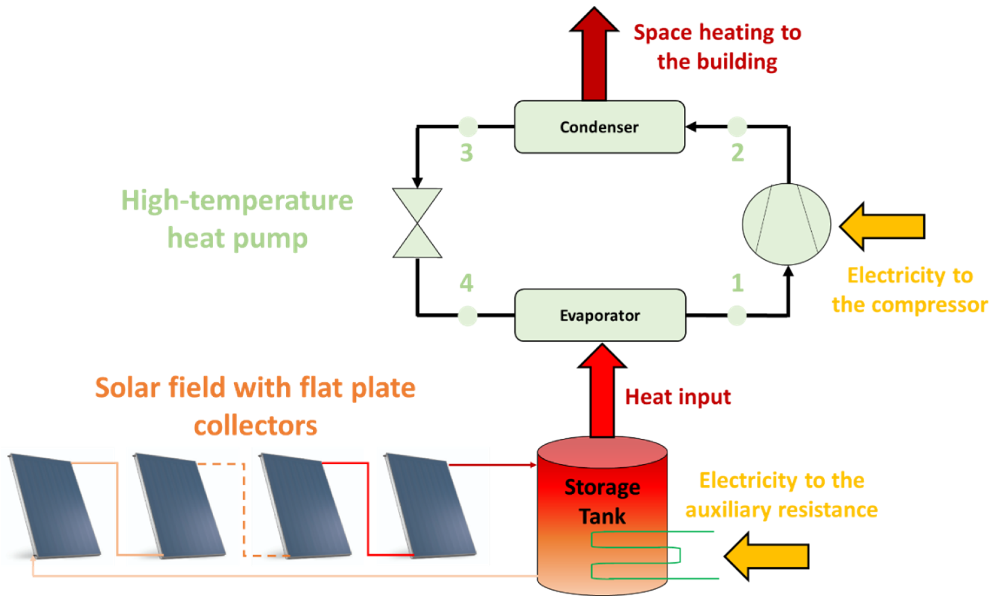
2.1. The Examined Configuration

The present work examines a solar-assisted heat pump with an auxiliary resistance and a thermal storage tank for producing space heating at high temperatures for feeding properly radiative terminal units. Figure 1 illustrates the studied solar-assisted heat pump space heating system. It is clear that the flat-plate collectors are used for producing useful heat at low temperatures which feeds the thermal storage tank. The tank includes an electrical thermal resistance of 5 kW which is used for keeping the working medium temperature over 12 °C. This design makes it possible (i) to avoid any freezing issues and (ii) to achieve adequate COP in the heat pump throughout the year period. The working medium in the solar field was selected to be water/glycol (50–50%). It is useful to state that the analysis is conducted for the heating period which starts on the 1st of November and stops on the 30th of April. The high-temperature heat pump uses the environmentally friendly working fluid R1234ze(E) which has zero ODP and a GWP of 6, while it is not toxic and it has an acceptable flammability (A2L—ASHRAE safety Classification) [24].

In this work, flat-plate collectors at 45° are chosen to have suitable solar irradiation exploitation in the winter period. This slope is a suitable one for the city of Athens, Greece, with a latitude equal to 38°. The solar thermal system stores heat in an insulated thermal storage tank which presents an overall thermal loss coefficient equal to 0.5 W/m²K [25]. The solar field collecting area (A_col) and the tank’s volume (V) are design parameters in this work, and they are examined parametrically.

The heat pump is a high-temperature device that produces heat at 70 °C (condenser temperature). The compressor of this system is selected to be the “2EES-3Y-40S” from the Bitzer company [26]. The superheating in the evaporator outlet is 10 K, while there is no subcooling in the condenser outlet. The compressor’s isentropic efficiency was extracted by using data from the Bitzer software v6.18.0 [27].

The heating loads of this study regard a building in Athens (Greece) and they are calculated by the TRNSYS software v18.02.2 [22]. The examined building is created according to the minimum requirements of the Greek regulation (KENAK) [28] for the buildings in climate zone B where Athens belongs. The floor area of the examined building is equal to 225 m² with a height of 3 m. The south wall includes an opening of an 8 m² area which is covered with a double-glazed window of U_w = 2.6 W/m²K [28] and a g-value of 0.75. Each external wall has a U-value of 0.45 W/m²K, the roof has a U-value of 0.40 W/m²K and the ground has a U-value of 0.40 W/m²K [28]. All the external structural components of the building come in contact with the ambient air. The sum of infiltration and natural ventilation rates is equal to one air change per hour, the specific equipment load is chosen at 4 W/m² and the specific lighting load at 3 W/m². The building is a residential one with four occupants with a specific load of 100 W/person [29]. The indoor temperature is properly controlled in order to be over 20 °C during the heating period which starts in November and lasts up to the end of April.

2.2. Mathematical Modeling Part

This part includes the most important formulas which describe the behavior of the examined system. These equations concern the modeling of the solar collectors, the storage tank, the heat pump and the overall system evaluation.

2.2.1. Solar Field and Storage Tank Modeling

The solar thermal efficiency of the FPC (η_col) is given by the next expression [30]:

$${\mathsf{\eta }}_{\mathrm{col}}=0.80-3.56\cdot \frac{{\mathrm{T}}_{\mathrm{m}}-{\mathrm{T}}_{\mathrm{am}}}{{\mathrm{G}}_{\mathrm{T}}}-0.003\cdot \frac{{\left({\mathrm{T}}_{\mathrm{m}}-{\mathrm{T}}_{\mathrm{am}}\right)}^2}{{\mathrm{G}}_{\mathrm{T}}}$$

(1)

The mean working fluid temperature (T_m), the ambient temperature (T_am) and the solar irradiation on the collector-tilted plane (G_T) are used in the previous formula.

The useful thermal product of the FPC (Q_u) can be calculated as below:

$${\mathrm{Q}}_{\mathrm{u}}={\mathsf{\eta }}_{\mathrm{col}}\cdot {\mathrm{Q}}_{\mathrm{sol}}$$

(2)

The available solar energy (Q_sol) is calculated according to the following formula:

$${\mathrm{Q}}_{\mathrm{sol}}={\mathrm{G}}_{\mathrm{T}}\cdot {\mathrm{A}}_{\mathrm{col}}$$

(3)

The fluid outlet temperature of the solar field (T_out) is found by the next expression:

$${\mathrm{T}}_{\mathrm{out}}={\mathrm{T}}_{\mathrm{in}}+\frac{{\mathrm{Q}}_{\mathrm{u}}}{\mathrm{m}\cdot {\mathrm{c}}_{\mathrm{p}}}$$

(4)

The working medium mass flow rate (m) in the solar field is selected to follow the next empirical expression [31]:

$$\mathrm{m}=0.02\cdot {\mathrm{A}}_{\mathrm{col}}$$

(5)

Moreover, it is useful to add that the fluid’s mean temperature (T_m) can be calculated as below:

$${\mathrm{T}}_{\mathrm{m}}=\frac{{\mathrm{T}}_{\mathrm{in}}+{\mathrm{T}}_{\mathrm{out}}}{2}$$

(6)

The thermal energy balance in the insulated tank is given below [32]:

$${\mathrm{Q}}_{\mathrm{st}}={\mathrm{Q}}_{\mathrm{u}}+{\mathrm{Q}}_{\mathrm{aux}}-{\mathrm{Q}}_{\mathrm{loss}}-{\mathrm{Q}}_{\mathrm{hp}}$$

(7)

The stored energy in the working fluid of the tank (Q_st) can be expressed by using the tank volume (V), the fluid density (ρ) and the fluid’s specific heat capacity (c_p):

$${\mathrm{Q}}_{\mathrm{st}}=\mathsf{\rho }\cdot \mathrm{V}\cdot {\mathrm{c}}_{\mathrm{p}}\cdot \frac{{\mathrm{dT}}_{\mathrm{st}}}{\mathrm{dt}}$$

(8)

The tank thermal loss (Q_loss) can be calculated by using the thermal loss coefficient (U_T), the tank’s external area (A_T), the tank’s mean temperature (T_st) and the ambient temperature (T_am) [32]:

$${\mathrm{Q}}_{\mathrm{loss}}={\mathrm{A}}_{\mathrm{T}}\cdot {\mathrm{U}}_{\mathrm{T}}\cdot \left({\mathrm{T}}_{\mathrm{st}}-{\mathrm{T}}_{\mathrm{am}}\right)$$

(9)

The auxiliary heat input (Q_aux) is activated when the tank’s mean temperature is (T_st < 12 °C) and it tries to make the fluid reach 12 °C with a proper control system. The maximum capacity of the auxiliary system is 5 kW.

The heat input rate in the evaporator (Q_hp) is dependent on the heating demand and it can be expressed as below:

$${\mathrm{Q}}_{\mathrm{hp}}={\mathrm{Q}}_{\mathrm{heat}}\cdot \frac{{\mathrm{COP}}_{\mathrm{hp}}-1}{{\mathrm{COP}}_{\mathrm{hp}}}$$

(10)

The building’s heating load of the building (Q_heat) was calculated by the simulation in the TRSNSYS tool, while the performance of the heat pump (COP_hp) was calculated by the thermodynamic analysis by the developed code in Engineering Equation Solver.

2.2.2. High-Temperature Heat Pump Modeling

The heat pump’s modeling is based mainly on the use of energy balances in the devices of the heat pump separately.

The heat input rate in the evaporator device from the solar field (Q_hp) can be written as

$${\mathrm{Q}}_{\mathrm{hp}}={\mathrm{m}}_{\mathrm{hp}}\cdot \left({\mathrm{h}}_1-{\mathrm{h}}_4\right)$$

(11)

The temperature of the state point (1) is found as below:

$${\mathrm{T}}_1={\mathrm{T}}_{\mathrm{evap}}+{\mathsf{\Delta }\mathsf{{\rm T}}}_{\mathrm{sh}}$$

(12)

The superheating in the present work is selected to be at ΔΤ_sh = 10 K. Moreover, the minimum temperature difference in the evaporator between the two streams is chosen to be at 5 K.

The condenser device is responsible for the heating load production (Q_heat):

$${\mathrm{Q}}_{\mathrm{heat}}={\mathrm{m}}_{\mathrm{hp}}\cdot \left({\mathrm{h}}_2-{\mathrm{h}}_3\right)$$

(13)

The fluid in the condenser outlet is selected to be saturated liquid because there is no subcooling in the present study. Moreover, in the main analysis, the condenser temperature is selected at T_cond = 70 °C in the present work to be able to feed radiative terminal units for heating.

The electricity demand in the heat pump’s compressor (P_el,com) can be found below:

$${\mathrm{P}}_{\mathrm{el},\mathrm{com}}={\mathrm{m}}_{\mathrm{hp}}\cdot \left({\mathrm{h}}_2-{\mathrm{h}}_1\right)$$

(14)

The compression process is modeled with the isentropic efficiency (η_is). This parameter is expressed with the next formula:

$${\mathsf{\eta }}_{\mathrm{is}}=\frac{{\mathrm{h}}_{2,\mathrm{is}}-{\mathrm{h}}_1}{{\mathrm{h}}_2-{\mathrm{h}}_1}$$

(15)

The state point (2,is) is found by the intersection of the isentropic line of s = s₁ with the line of high-pressure p = p_h. More details regarding the modeling of the isentropic efficiency can be found in Ref. [33].

The pressure reduction in the throttling valve is performed in an ideal way and thus it can be written as

$${\mathrm{h}}_4={\mathrm{h}}_3$$

(16)

The definition coefficient of performance (COP_hp) for heating production in the heat pump is given according to the next formula:

$${\mathrm{COP}}_{\mathrm{hp}}=\frac{{\mathrm{Q}}_{\mathrm{heat}}}{{\mathrm{P}}_{\mathrm{el},\mathrm{com}}}$$

(17)

At this point, it has to be added that there is an extra electricity consumption from the auxiliary electrical resistance (P_el,aux). Therefore, the total electricity (P_el,tot) consumption can be written as below:

$${\mathrm{P}}_{\mathrm{el},\mathrm{tot}}={\mathrm{P}}_{\mathrm{el},\mathrm{com}}+{\mathrm{P}}_{\mathrm{el},\mathrm{aux}}$$

(18)

The system’s coefficient of performance (COP_sys) is given according to the next expression:

$${\mathrm{COP}}_{\mathrm{sys}}=\frac{{\mathrm{Q}}_{\mathrm{heat}}}{{\mathrm{P}}_{\mathrm{el},\mathrm{tot}}}$$

(19)

2.2.3. Evaluation Metrics

The yearly heating energy demand (E_heat) is calculated according to the next expression:

$${\mathrm{E}}_{\mathrm{heat}}={{\displaystyle \int }}_{\mathrm{October}}^{\mathrm{April}}{\mathrm{Q}}_{\mathrm{heat}}\cdot \mathrm{dt}$$

(20)

The yearly electricity demand (E_el) is calculated as below:

$${\mathrm{E}}_{\mathrm{el},\mathrm{tot}}={{\displaystyle \int }}_{\mathrm{October}}^{\mathrm{April}}{\mathrm{P}}_{\mathrm{el},\mathrm{tot}}\cdot \mathrm{dt}$$

(21)

The yearly (or seasonal) coefficient of performance (SCOP) of the system can be found as below:

$$\mathrm{SCOP}=\frac{{\mathrm{E}}_{\mathrm{heat}}}{{\mathrm{E}}_{\mathrm{el},\mathrm{tot}}}$$

(22)

The life cycle cost (LCC) of the investment is calculated according to the following expression:

$$\mathrm{LCC}=\mathrm{CC}+{{\displaystyle \sum }}_{\mathrm{i}=1}^{\mathrm{N}}\frac{{\mathrm{E}}_{\mathrm{el}}\cdot {\mathrm{k}}_{\mathrm{el}}+\left(\mathrm{O}\&\mathrm{M}\right)}{{\left(1+\mathrm{r}\right)}^{\mathrm{i}}}$$

(23)

In this work, the capital cost includes the cost of the solar field, the thermal tank and the heat pump. The specific cost of the solar field was elected at 150 EUR/m² [32], of the storage tank at 1000 EUR/m³ [34] and of the heat pump at 750 EUR/kW_th [35] (the maximum thermal load of the building was found at 6 kW according to the simulation in TRNSYS). Moreover, the yearly operation and maintenance cost (O&M) was chosen to be 1% of the investment cost [36]. The investment lifetime was selected at N = 25 years and the discount factor at r = 3%. The electricity was estimated at k_el = 0.22 EUR/kW_el by taking into consideration the new increases in the electricity price.

2.3. Description of the Methodology Path

The goal of this work is the yearly analysis of a solar-assisted heat pump heating system. A building in Athens, Greece (37°59′ N, 23°43′ E), with a 225 m² floor area is examined and its heating loads were calculated with a model in the TRNSYS tool [22]. A high-temperature heat pump was examined thermodynamically with a created model in Engineering Equation Solver [23]. Data from the Bitzer manufacturer were used to determine the isentropic efficiency of the compressor for the different operating scenarios. It is remarkable that the isentropic efficiency was found to range from 50% to 67%. A comparison of the heat pump COP with the Bitzer data proved a mean deviation of 0.8% which indicates the high accuracy of the developed mode. More details regarding the validity of the present model for the heat pump can be found in Ref. [33]. The next step was the COP approximation with a polynomial in order to develop an accurate formula for further use. Section 3.1 includes the developed formula and its evaluation procedure.

The final step was the development of a dynamic code in a homemade program for simulating the dynamic behavior of the total system. The weather data from the TRNSYS were used, and the heating demand of the simulation was inserted in the code. An assumption of the model is based on the satisfaction of the building loads during the heating period (October to April according to the simulation analysis). The dynamic model was based on the solution of the differential equation of the storage tank’s energy balance. The heat pump performance was modeled by the use of the approximation formula, as it was previously described. The goal is to connect the high-temperature heat pump with radiators and thus the condenser temperature was selected at 70 °C. This temperature level makes the operation of radiators possible, with a slightly lower temperature level compared to other systems. However, the selection of the condenser temperature at 70 °C and not at a greater temperature makes the efficient heat pump operation possible. It is also useful to add that there is an auxiliary electrical thermal resistance inside the storage tank (5 kW capacity) which make it possible to keep the mean tank temperature over 12 °C and also helps the heat pump to operate with a greater evaporator’s temperature and consequently with higher COP. The activation of the auxiliary resistance is seldom, and it takes place during the coldest days of the year with restricted solar potential.

The dynamic part of this study is presented in detail for the representative case with A_col = 30 m² and V = 3 m³. Moreover, the yearly evaluation indexes of the system are given for different combinations of solar field areas and tank volumes. More specifically, the collecting area is varied from 10 to 50 m², while the tank volume is from 1 to 5 m³. The system that leads to the lowest LCC was found to be the most appropriate one. Moreover, an extra multi-objective optimization procedure was applied by using two goals: (i) the minimization of the LCC and the maximization of the SCOP. The global optimum choice was found after using the criterion of the minimum dimensionless geometrical distance between the ideal point and the Pareto Front points. More specifically, the goal of the multi-objective optimization procedure was to minimize the following expression:

$$\mathrm{F}=\sqrt{{\left(\frac{{\mathrm{SCOP}}_{\max }-\mathrm{SCOP}}{{\mathrm{SCOP}}_{\max }-{\mathrm{SCOP}}_{\min }}\right)}^2+{\left(\frac{\mathrm{LCC}-{\mathrm{LCC}}_{\min }}{{\mathrm{LCC}}_{\max }-{\mathrm{LCC}}_{\min }}\right)}^2}$$

(24)

where the (min) and the (max) subscripts concern the minimum and the maximum obtained values, respectively, among the different studied scenarios. Every case is a different combination of collecting area and storage tank volume. Practically, these two parameters are the optimization parameters of the present analysis.

3. Results

The present section includes the results of the simulation investigation. The first step in Section 3.1 is the presentation of the heat pump performance, and the next part in Section 3.2 is devoted to the dynamic analysis of the unit. The last part of this section (Section 3.3) concerns the results of the parametric investigations and of the optimization.

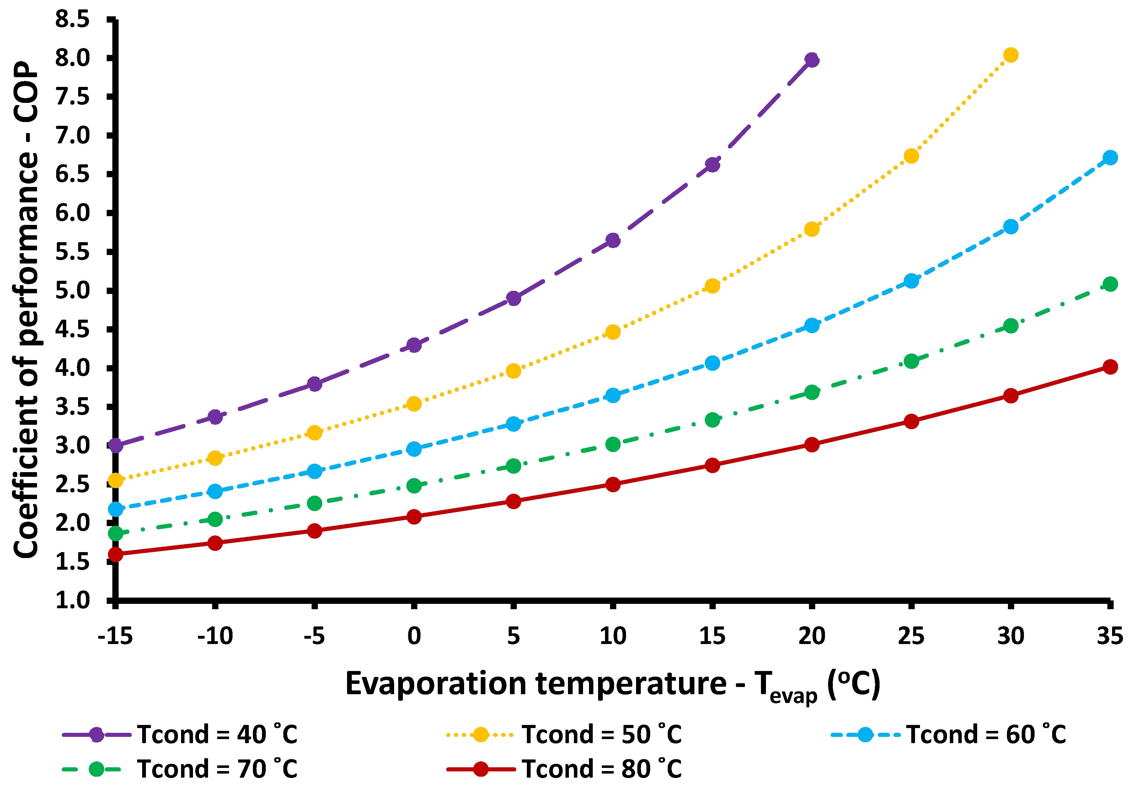
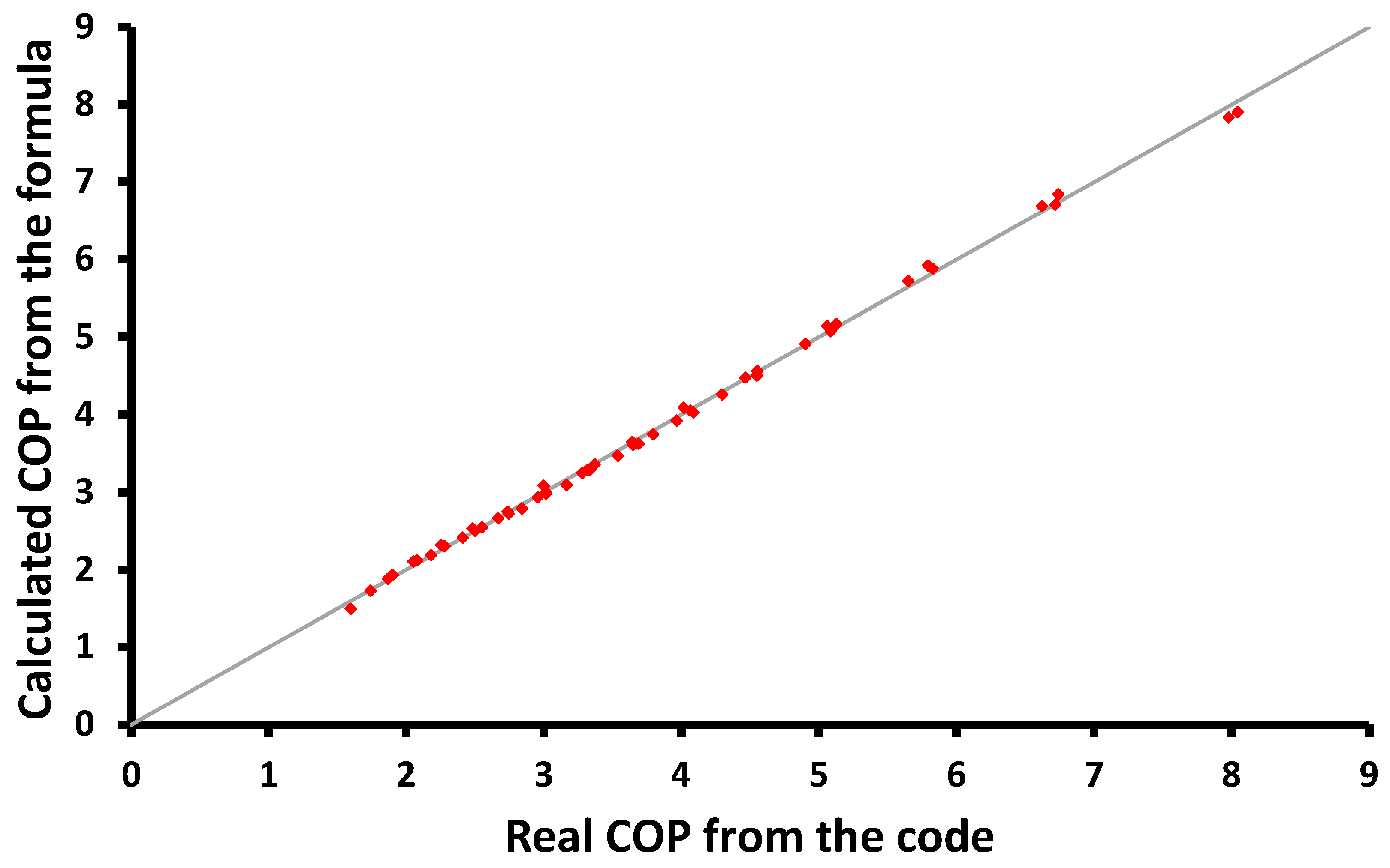
3.1. Heat Pump Investigation

The energy behavior of the high-temperature heat pump is presented in Figure 2 for different combinations of the temperature levels in the evaporator and in the condenser devices. It is obvious that the COP_hp increases with the evaporator temperature increase and it also increases with the condenser temperature reduction. The aforementioned behavior is reasonable because the COP_hp of the heat pump increases when there is a lower difference between the temperatures of the condenser and the evaporator devices. For the condenser temperature of 70 °C, the maximum COP_hp is found at 5.087 for T_evap = 35 °C, while the minimum is 1.867 for T_evap = −15 °C.

The COP is approximated with a polynomial expression which is given in Equation (25) by using the (T_cond) and the (T_evap) as parameters. The mean deviation of the Equation (25) results and the real calculated values by the code in Engineering Equation Solver were found at 1.21% which is a relatively low value. Thus, Equation (25) can be accepted as a reliable approximation for estimating the heat pump’s efficiency.

$$\begin{array}{c}\mathrm{COP}=12.61-0.3556·{\mathrm{T}}_{\mathrm{cond}}+4.538·{10}^{-3}·{\mathrm{T}}_{\mathrm{cond}}^2-2.165·{10}^{-5}·{\mathrm{T}}_{\mathrm{cond}}^3+0.3427·{\mathrm{T}}_{\mathrm{evap}}+9.962·{10}^{-3}·\\ {\mathrm{T}}_{\mathrm{evap}}^2+1.69·{10}^{-5}·{\mathrm{T}}_{\mathrm{evap}}^3-7.495·{10}^{-3}·{\mathrm{T}}_{\mathrm{cond}}·{\mathrm{T}}_{\mathrm{evap}}-2.314·{10}^{-4}·{\mathrm{T}}_{\mathrm{cond}}·{\mathrm{T}}_{\mathrm{evap}}^2+4.592·{10}^{-5}·{\mathrm{T}}_{\mathrm{cond}}^2·\\ {\mathrm{T}}_{\mathrm{evap}}+1.364·{10}^{-6}·{\mathrm{T}}_{\mathrm{cond}}^2·{\mathrm{T}}_{\mathrm{evap}}^2\end{array}$$

(25)

Moreover, it has to be added that the approximation equation is valid for the following conditions:

$$40°\mathrm{C}\le {\mathrm{T}}_{\mathrm{cond}}\le 80°\mathrm{C}\hspace{1em}\mathrm{and}\hspace{1em}-15°\mathrm{C}\le {\mathrm{T}}_{\mathrm{cond}}\le 35°\mathrm{C}$$

However, in the case of T_cond = 40 °C, the maximum evaporator temperature is T_evap,max = 20 °C, while in the case of T_cond = 50 °C, the maximum evaporator temperature is T_evap,max = 30 °C.

Figure 3 illustrates the COP calculated with the code and with the aforementioned equation, and it is clear that the results are very close to each other. This fact validates the high accuracy of the approximation expression.

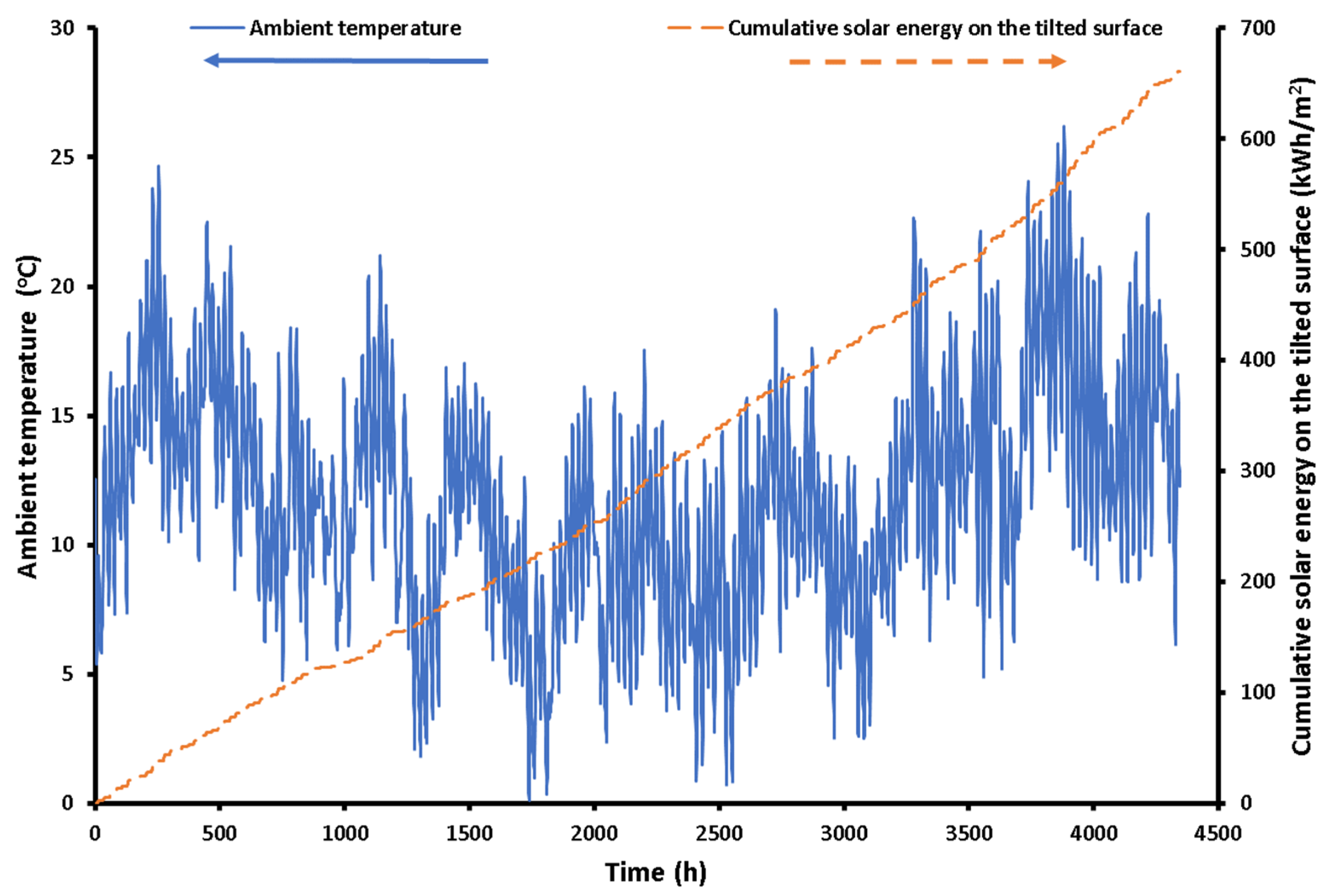
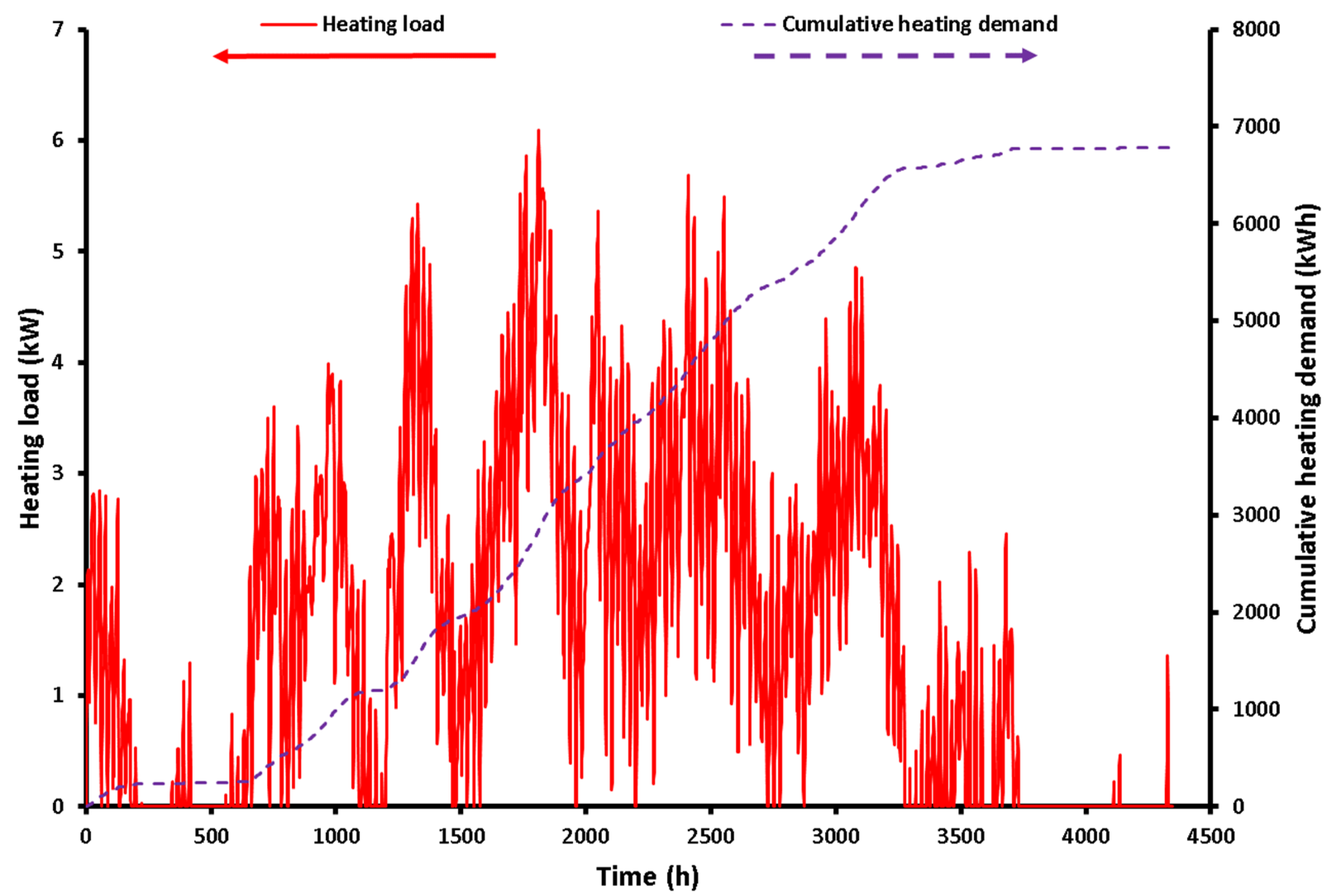
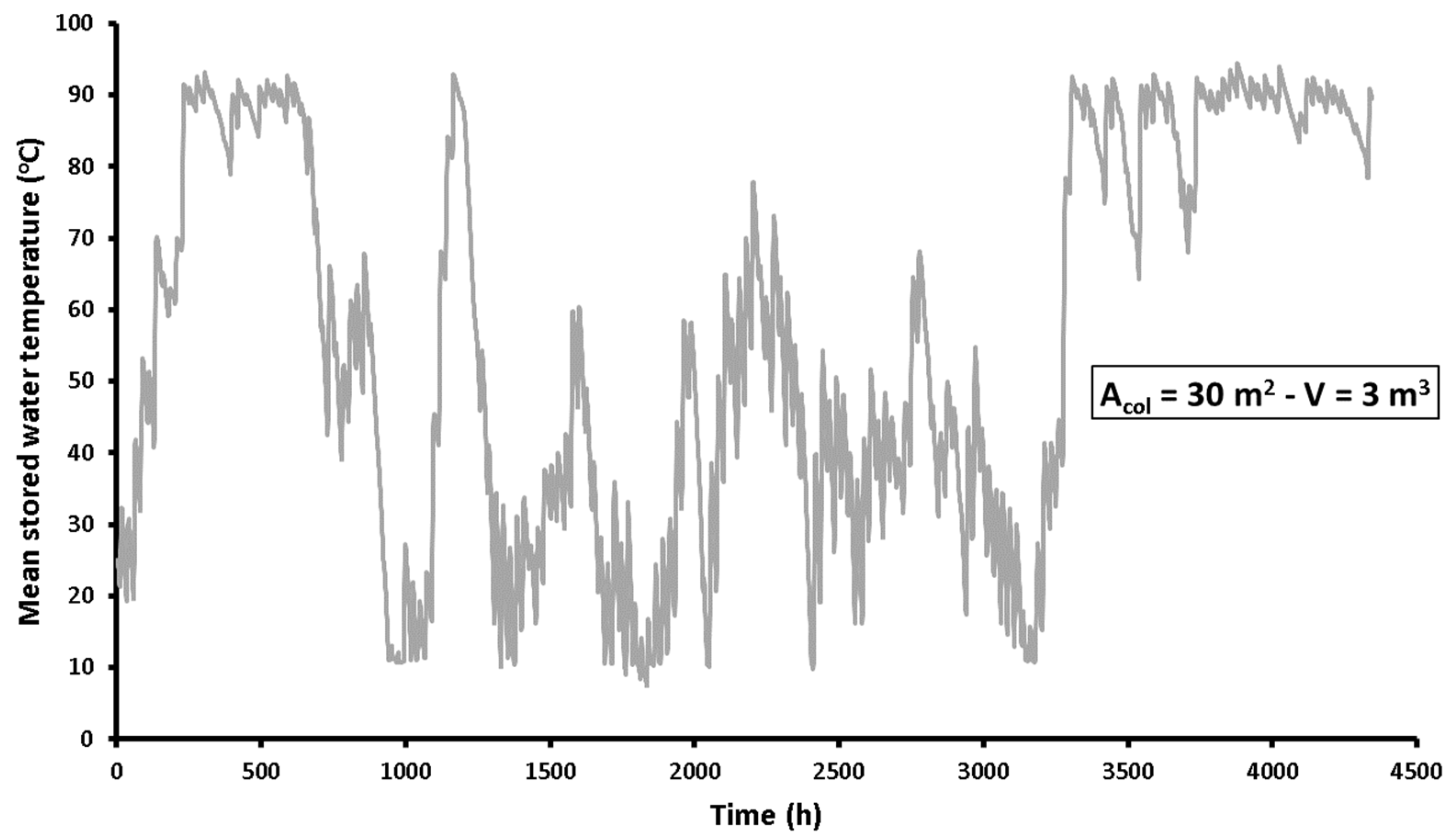
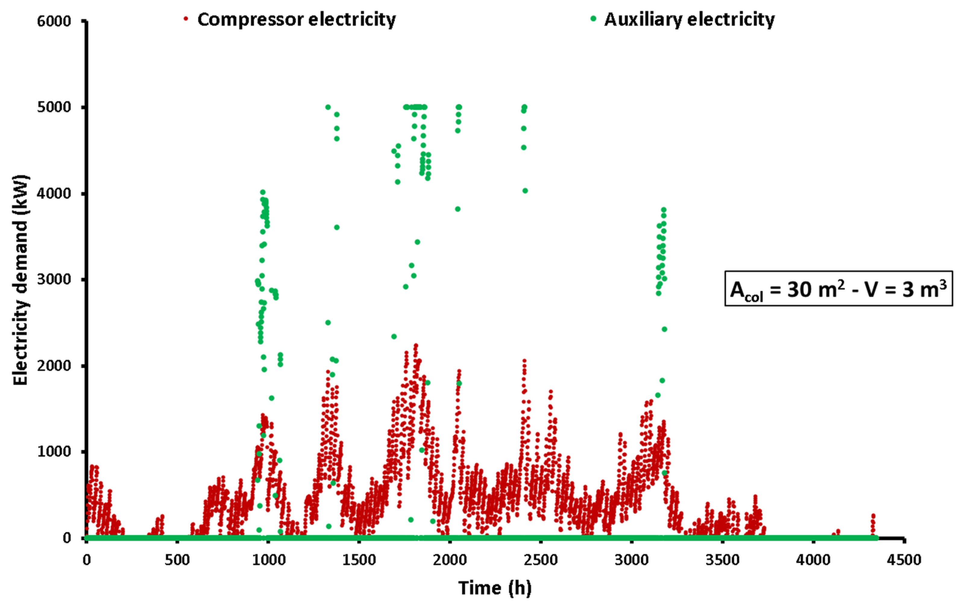
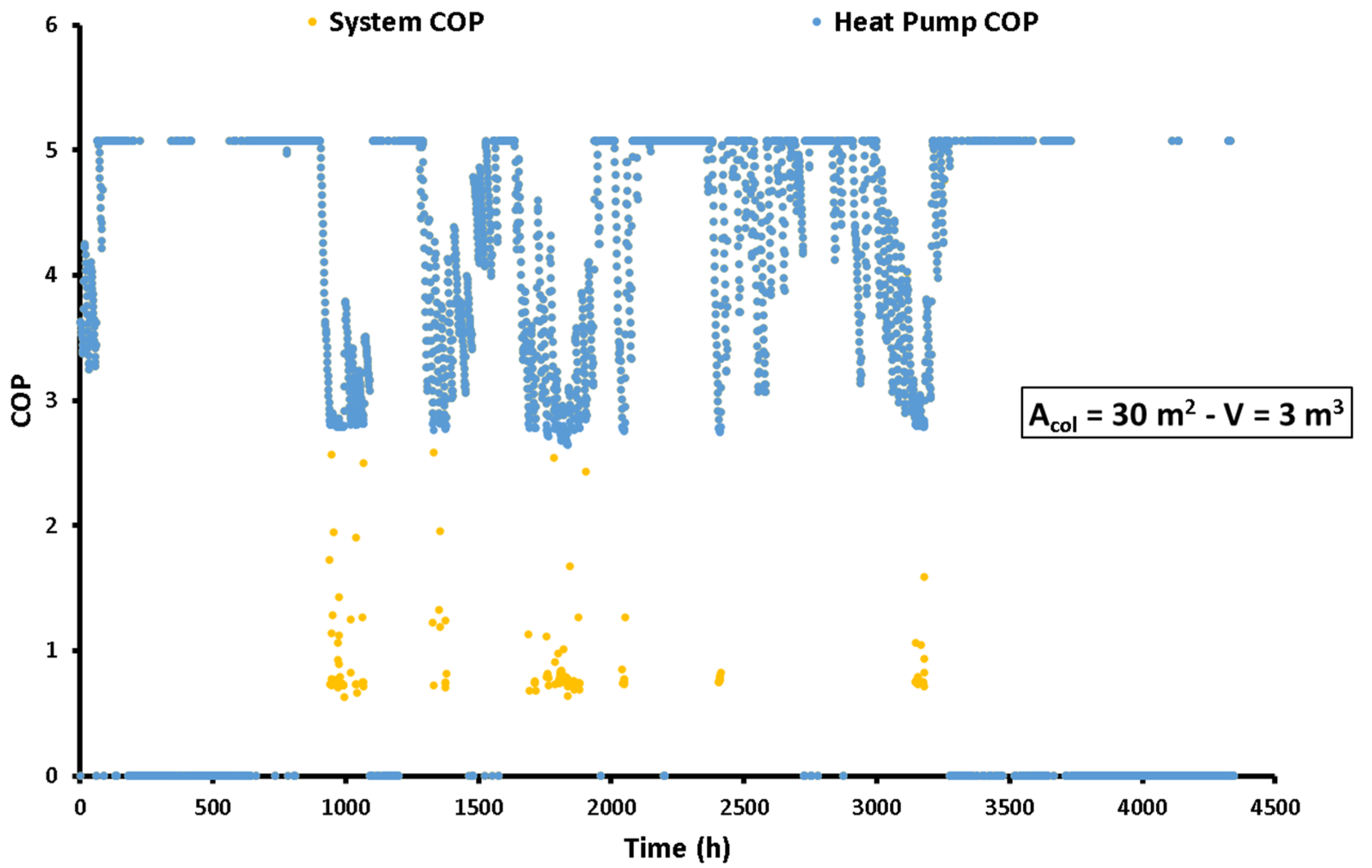
3.2. Dynamic Analysis of the System

The results of the dynamic analysis for the heating period (October to April) are included in this section. It is interesting to say that these results are given for a representative design case A_col = 30 m² and V = 3 m³ in order to show how the system behaves during the different heating needs.

The first step in this investigation is the presentation of the weather data of the examined city. Figure 4 shows the variation in the ambient temperature during the heating period, as well as the cumulative solar irradiation on the tilted surface per area for the heating period. It is clear that the minimum ambient temperature is about 0 °C while the solar potential is 661 kWh/m². These results show that in the examined location, (i) there are no extremely low ambient temperature levels, (ii) there are significant heating needs and (iii) there is adequate solar potential for solar thermal technology utilization.

Figure 5 depicts the heating demand expressed in terms of power (kW) and in terms of cumulative energy (kWh). The maximum heating load is calculated close to 6 kW and the seasonal heating demand is at 6785 kWh. Moreover, it is useful to state that the coldest period in Greece is the months of December, January and February, while April presents restricted heating loads.

The next stage is the presentation of the system performance results during the winter period. Figure 6 illustrates the variation in the mean tank temperature during the heating season. The minimum obtained temperature is around 10 °C due to the activation of the auxiliary system when lower values are obtained. Moreover, the maximum temperature in the tank is 95 °C because there is a proper control system to stop the collector operation when this limit is reached. The low temperatures in the tank are found in the period of high heating loads, while in the period of low heating loads the tank temperature increases. Moreover, it is significant to add that the low heating loads are usually associated with increased solar potential, something that makes it possible on some days to have a very high solar potential and a very small heating demand. These facts justify the increase in the tank temperature up to 95 °C. These relatively high values are detected in the months with a relatively small heating demand (November, March and April). More specifically, on days of low heating loads, the tank temperature increases because there is higher useful heat production from the solar system than the heat input demand in the heat pump. So, it is possible to transfer stored solar energy to the next days and to assist them in the case of increased heating needs on them.

Figure 7 depicts the electricity consumption during the heating period which is consumed by the compressor and by the auxiliary electrical heater. It is useful to note that the auxiliary electrical resistance is activated when the temperature of the stored water is very low, and its activation aims to keep it at 10–12 °C for a safe operation. Practically, the avoidance of the extremely low water temperature levels makes the efficient operation of the compressor possible and so the COP is kept at acceptable levels in the system’s overall daily cycle. It is obvious that the auxiliary heater is activated only in some restricted cases during the period, and more specifically, it operates for 187 h during the heating period. On the other hand, the heat pump operates for 3008 h; thus, the auxiliary system is activated only for 6.2% of the heating time. This fact indicates that the auxiliary system is the minor energy unit in the present system. The maximum electricity consumption in the compressor is found at 2.243 kW while the auxiliary system is at 5 kW. The maximum total electricity consumption was found at 7.243 kW at 10:00 on the 17 of February.

At the end of this subsection, Figure 8 exhibits the variation in the COP during the year for the heat pump and for the unit. The difference between these two indexes is based on the use of the auxiliary electrical resistance for some hours during the year and this fact makes the COP_sys be decreased at these periods compared to the COP_hp. In the periods without activation of the electrical resistance, the two indexes (COP_sys and COP_hp) have the same values. The COP_hp ranges between 2.65 and 5.08, with the lowest values obtained when the tank water is relatively cold. The COP_sys ranges from 0.69 to 5.08, with the lowest values obtained when the auxiliary electrical resistance is activated. It is useful to state that the auxiliary system is activated only for 187 h per year which corresponds to 6.2% of the total operating period. Thus, it is clear that for only a few cases the COP_sys takes low values (under 1), and the system is not so efficient. However, the given values of the COP_sys regard the instantaneous efficiency of the unit; this fact indicates that a quantity of the consumed electricity by the auxiliary system can increase the water temperature and assist the system in the near-future time periods, something that indicates that this design is a sustainable one.

3.3. Parametric Analysis and Optimization

The present section examines the yearly performance of the unit parametrically by presenting the results for different combinations of the design parameters. The solar field area and the thermal tank volume are the designed parameters that are studied in detail. Figure 9 shows the influence of the collecting area on critical energy quantities of the unit while the storage tank volume is equal to 3 m³ in this figure. A higher collecting area leads to a greater useful heat product from the solar field but with a decreasing rate. The decreasing rate is reasonable because a higher solar field area increases the mean operating temperature in the tank and therefore the solar efficiency is reduced. The increase in useful heat product practically gives the system a higher energy input and makes it possible to reduce the electricity consumption with the collecting area increase. This reduction is more intense in the auxiliary electrical consumption, while the compressor electricity consumption is decreased but not dramatically. More specifically, the auxiliary electrical consumption decreases from 3591 kWh to 210 kWh, while the compressor electricity consumption decreases from 5881 kWh to 1669 kWh.

Figure 10 depicts the influence of the tank’s volume on the crucial energy quantities of the system while the collecting area is equal to 30 m² in this figure. A larger storage tank’s volume makes the mean temperature of the fluid be reduced and so the thermal performance of the solar system is increased. This fact justifies the increase in the useful heat production of the solar field with the increase in the storage tank volume. Moreover, a higher storage tank capacity leads to smaller electricity consumption, especially by reducing the auxiliary electrical resistance consumption. The compressor consumption shows a very small reduction with the increase in the tank’s volume.

The next part of this work is the depiction of the results for different combinations of the two examined design parameters. Figure 11 illustrates the mean yearly solar thermal efficiency for the different studied cases. According to the results, a higher collecting area reduces the efficiency because greater useful heat production increases the mean operating temperature, something that leads to higher thermal losses in the solar system. Moreover, the increase in the storage tank volume can lead to a slightly higher collector thermal efficiency due to the decrease in the mean operating temperature in the system. The range of the yearly solar thermal efficiency is found to be from 20.91% (for A_col = 50 m² and V = 1 m³) to 64.54% (for A_col = 10 m² and V = 5 m³).

Figure 12 exhibits the impact of the total electricity demand for the different combinations of the collecting areas and tank capacities. It is clear that a higher solar field area reduces the electricity demand because there is a greater available heat input in the system. Moreover, a larger storage tank also reduces the electricity demand because a greater storage tank makes the most appropriate management of useful heat production possible. The range of the total electrical demand is calculated to be from 1503 kWh (for A_col = 50 m² and V = 5 m³) to 6112 kWh (for A_col = 10 m² and V = 1 m³).

The next step is the presentation of the auxiliary electricity percentage to the total electricity demand for the different cases, as Figure 13 depicts. It is obvious that an increase in the collecting area leads to a dramatic decrease in the auxiliary electricity percentage. Moreover, an increase in the storage tank volume leads to a significant decrease in the auxiliary electricity percentage. The range of the auxiliary electricity percentage is found to be from 4.92% (for A_col = 50 m² and V = 5 m³) to 62.26% (for A_col = 10 m² and V = 1 m³).

The system seasonal coefficient of performance (SCOP) is illustrated in Figure 14. It is clear that higher values of the collecting area and the tank’s volume lead the SCOP to receive higher values. It can be said that the design with a tank capacity of 1 m³ leads to a very small efficiency, while the use of collecting areas up to 20–25 m² lead also to low performance. The range of the SCOP is found to be from 1.11 (for A_col = 10 m² and V = 1 m³) to 4.513 (for A_col = 50 m² and V = 5 m³).

The financial evaluation of the unit is based on the calculation of the life cycle cost index, as it is given in Figure 15. The aim is to determine the design which minimizes the LCC in order to have an economically feasible design. For every storage tank capacity, there is a specific collecting area that minimizes the LCC, and it is 35 m² for all the tank volumes. The global minimum LCC is found at 22,694 EUR (for A_col = 35 m² and V = 2 m³). So, this design is the optimal configuration according to the financial criterion.

The last step is the multi-objective optimization of the unit by using both energy and economic criteria. More specifically, the energy criterion is the maximization of the SCOP, and the economic criterion is the minimization of the LCC. The ideal point is the one that presents the maximum SCOP and the minimum LCC [SCOP = 4.513, LCC = 22,694 EUR] and the objective is to determine the design that has the lowest dimensionless distance from this point. Figure 16 depicts the examined designs, and it can be said that there are many designs close to the ideal one. The most appropriate design, after conducting the evaluation procedure, was found to be the one with (A_col = 50 m² and V = 3 m³) which leads to [SCOP = 4.066, LCC = 24,084 EUR].

The previous analysis indicates that different criteria lead to different optimum solutions. The economic optimization indicates that the best design is the one with (A_col = 35 m² and V = 2 m³), while the multi-objective optimization (energy and economic) indicates that the optimum scenario is (A_col = 50 m² and V = 3 m³). The ratio of the collectors’ area to the tank’s volume was found at 17.5 m²/m³ and 16.7 m²/m³ which are similar values, and this fact indicates that the storage tank volume “follows” the selection of the collecting area value. It is remarkable to state that the optimum collecting area of 35 m² has a significant difference from that of the value of 50 m². This fact indicates that the selection of the optimization criteria plays an important role in the final selection of the installed collecting area. In the case where the economic parameter is the most valuable index, a lower collecting area of 35 m² has to be selected, while in the case where energy efficiency is important, a higher collecting area of 50 m² has to be chosen. Practically, a higher collecting area makes the efficiency be enhanced and this fact indicates that in the cases that the efficiency plays a critical role in the decision-making process, then higher collecting areas have to be selected.

Table 1. Summary of the results for the optimum designs.

Parameter	Economic Optimization (LCC Minimization)	Multi-Objective Optimization
Optimum collecting area	35 m2	50 m2
Optimum storage tank volume	2 m3	3 m3
Yearly solar thermal efficiency	31.60%	25.33%
System SCOP	2.947	4.066
Heat pump SCOP	4.125	4.651
LCC	22,694 EUR	24,084 EUR
Heating demand	6785 kWh	6785 kWh
Total electricity demand	2302 kWh	1669 kWh
Compressor electricity demand	1645 kWh	1459 kWh
Auxiliary electricity demand	657 kWh	210 kWh
Percentage of auxiliary demand	28.55%	12.59%

includes the results for the two optimum scenarios.

It is interesting to state that the optimum design according to the multi-objective optimization procedure leads to a significantly lower electricity demand for both the compressor and auxiliary electrical resistance. Moreover, in terms of the LCC, the difference is not high, and it is about 1390 EUR. In other words, the optimum solution from the multi-objective optimization procedure leads to a 6.1% cost increase, while there is a significant reduction in the electricity demand of 27.5%. Thus, it can be said that the sacrifice of 6.1% in cost leads to energy savings of 27.5% which is a satisfactory percentage. To conclude, the addition of a greater solar field seems to be a reasonable choice because the increase in the LCC is not so high compared to the gain in the system’s energy performance. However, land restrictions and other issues have to be considered in the final selection of the installed solar field in every case. Thus, the final selection of the optimum design has to be based on the multi-objective optimization procedure and by considering any specific constraints of the examined case study. For the present system, as an empirical rule, it could be said that the final heat pump COP could be estimated by using equation (25) for T_cond = 70 °C and T_evap = 31 °C in order to reach the value of SCOP = 4.651 approximately. This is an empirical rule which can estimate in a quick way the total SCOP of the system and it can be used for performing quick calculations for the design of future systems. Practically, in future solar-assisted heat pump heating systems, the final optimum SCOP could be calculated by using the inputs (T_evap = 31 °C and T_cond = 70 °C) for having a preliminary reasonable estimation.

3.4. Discussion and Future Steps

The present work investigates a system with a high-temperature heat pump coupled with solar thermal systems which can be an alternative answer to the existing space heating systems. This idea has important benefits such as (i) the exploitation of renewable energies, (ii) the use of environmentally friendly refrigerants, (iii) the use of highly efficient heat pumps and (iv) the incorporation of radiative terminal units for achieving high thermal comfort standards. Moreover, the present system has a positive impact on various sustainable development goals and more specifically on “Affordable and clean energy”, “Sustainable cities and communities” and “Climate action”.

The high efficiency of the solar-assisted system compared to the air-source system can be found by comparing the existing results of the optimum scenario with the results of our previous work in Ref. [33]. More specifically, the system SCOP is found in this work at 4.066, while in the previous work, it was 2.128 [33]; so, there is a significant enhancement with the use of a solar-assisted system. However, the present system needs the installation of a solar field which adds an extra cost. In the future, it would be very interesting to investigate a dual-source heat pump that can be driven both with air and solar in order to avoid the use of the auxiliary electrical resistance of the present system or to restrict it.

To conclude, in the future, it is important to investigate the present system under different climate conditions and by optimizing the radiative terminal units in order to be suitable for the present configuration. Moreover, the use of a model predictive control unit would be very interesting in order to optimize the examined system by taking into account the weather data of the next days and properly adjusting the thermal stored energy.

4. Conclusions

Solar-assisted heat pump heating units are promising choices for providing the space heating demand with reasonable electricity consumption. The present work examines such a configuration with a high-temperature heat pump aiming to provide high-temperature heat for feeding radiative terminal units. The analysis is conducted for a typical case study of a building in Athens (Greece). The most valuable conclusions of the present investigation are the following:

-

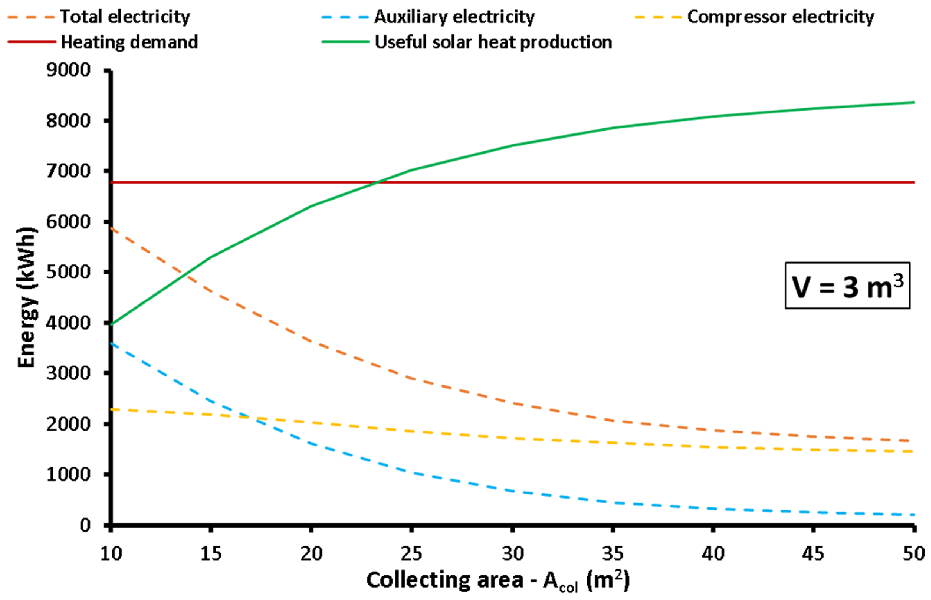
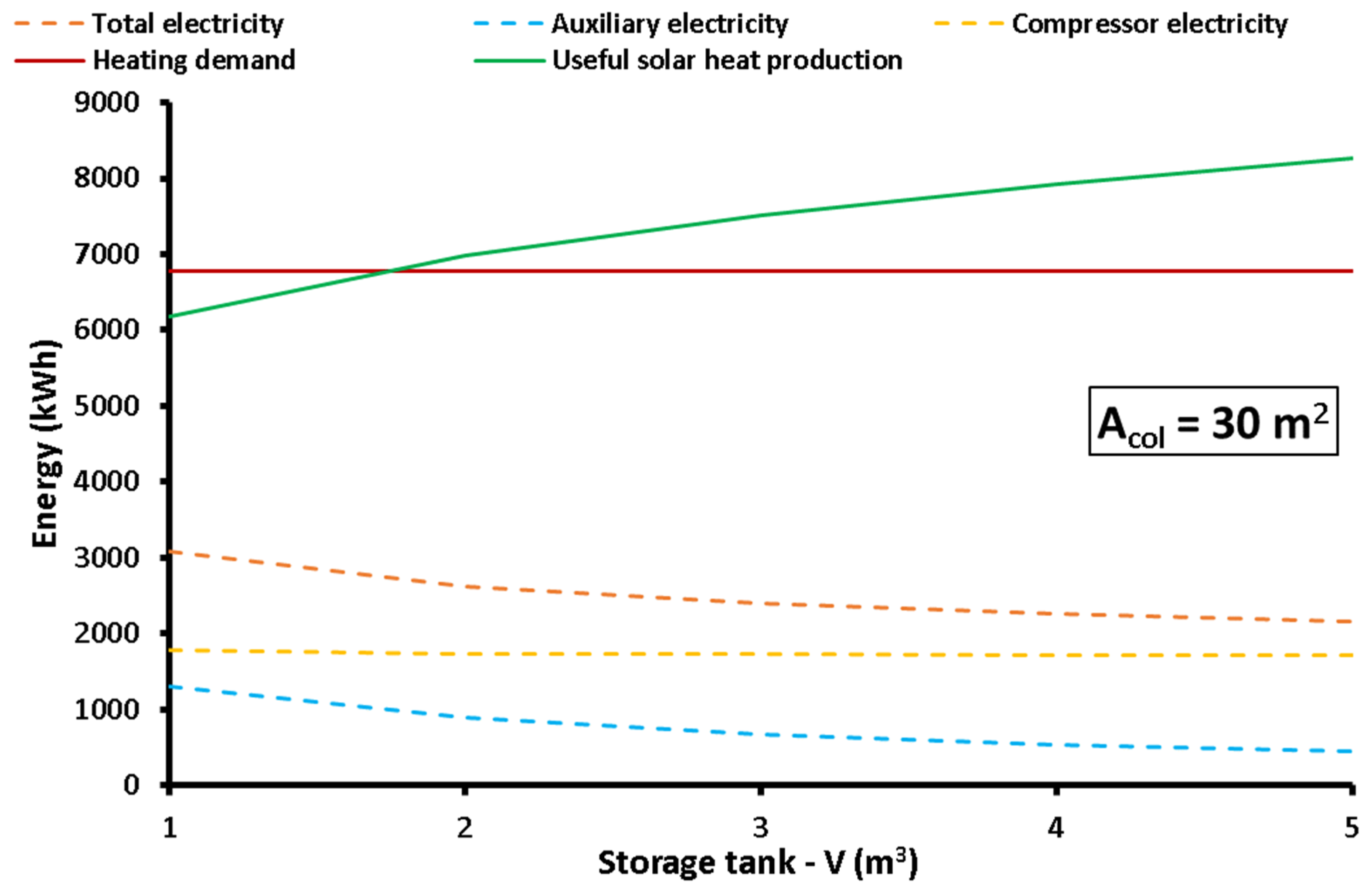
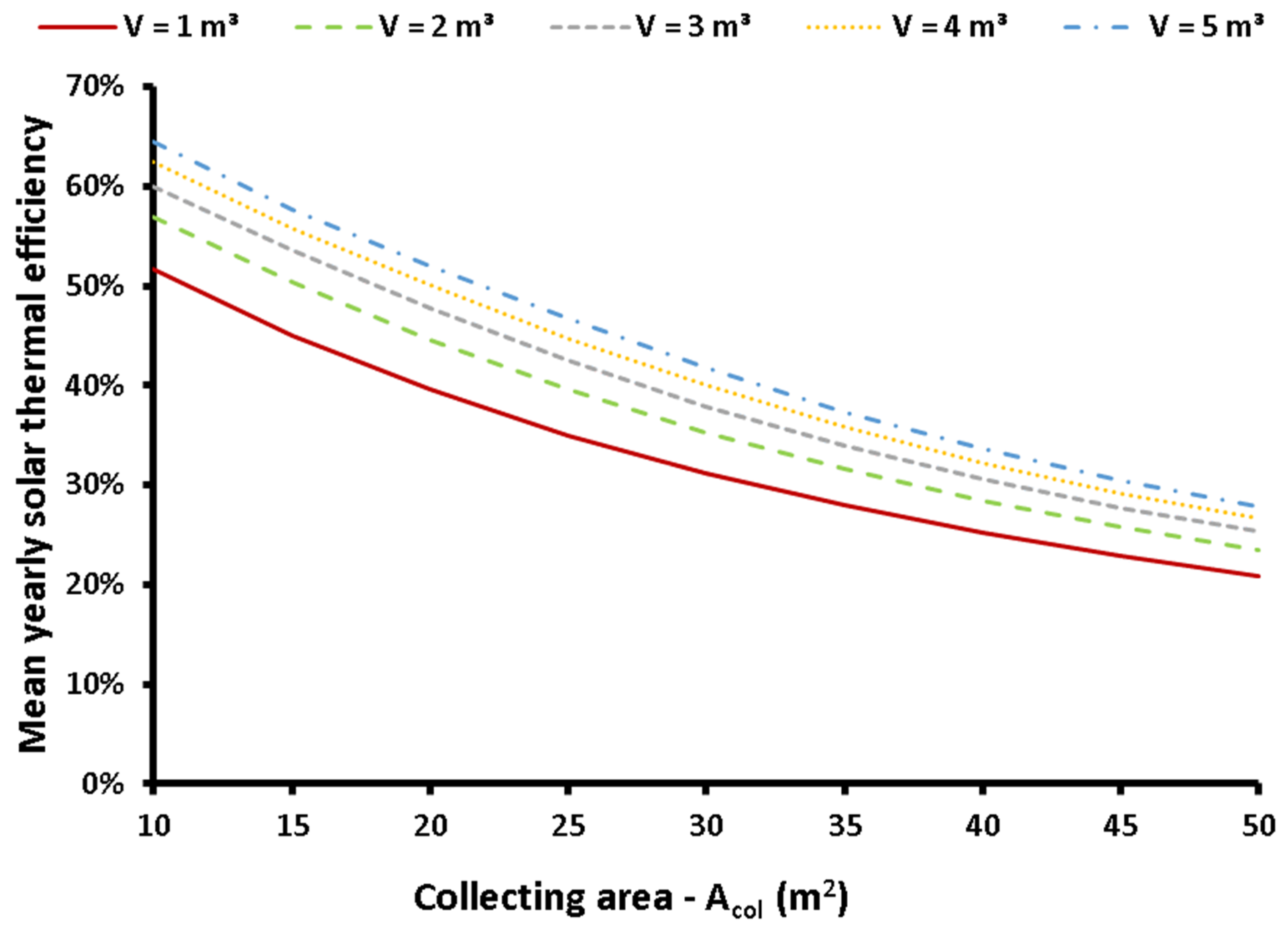
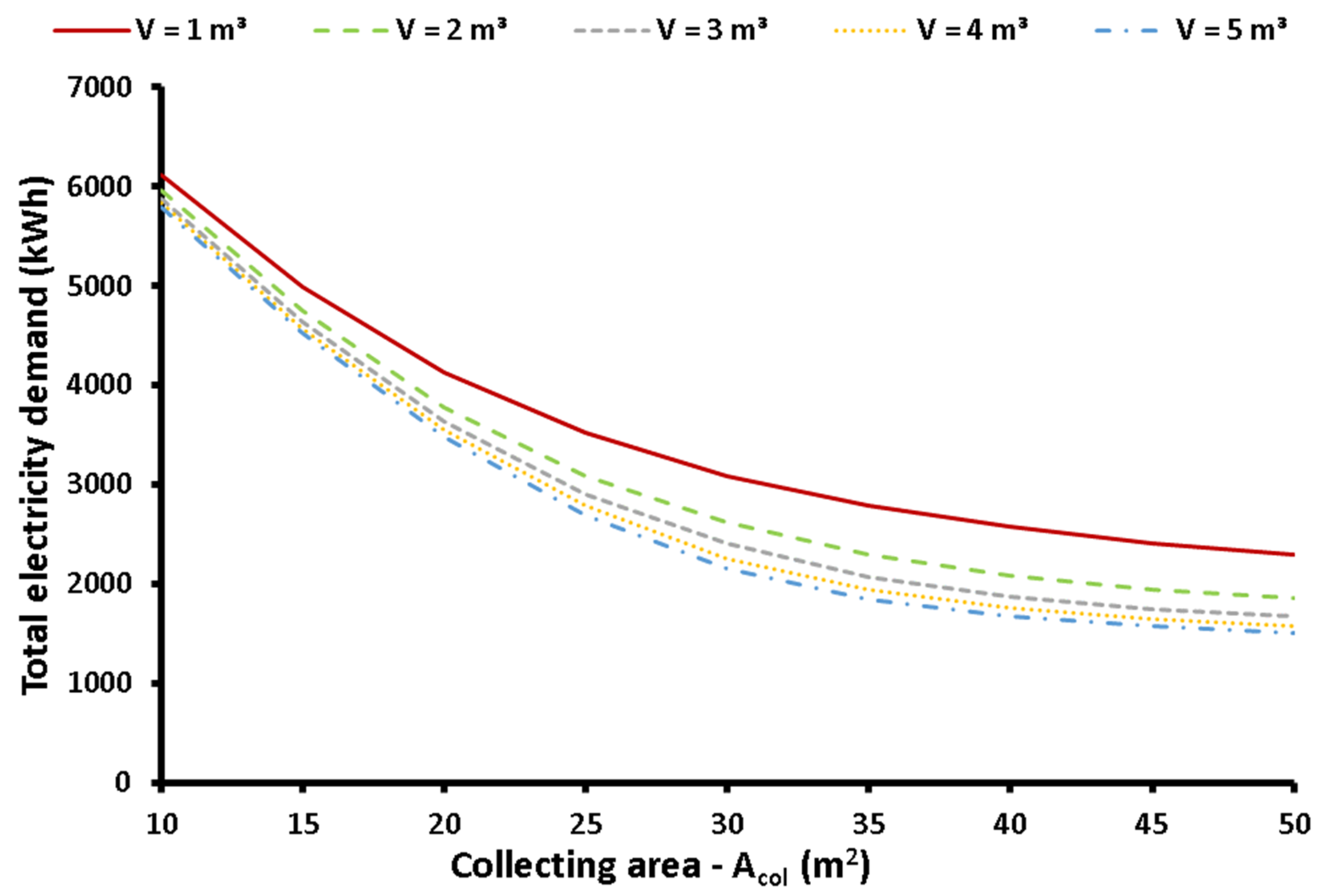
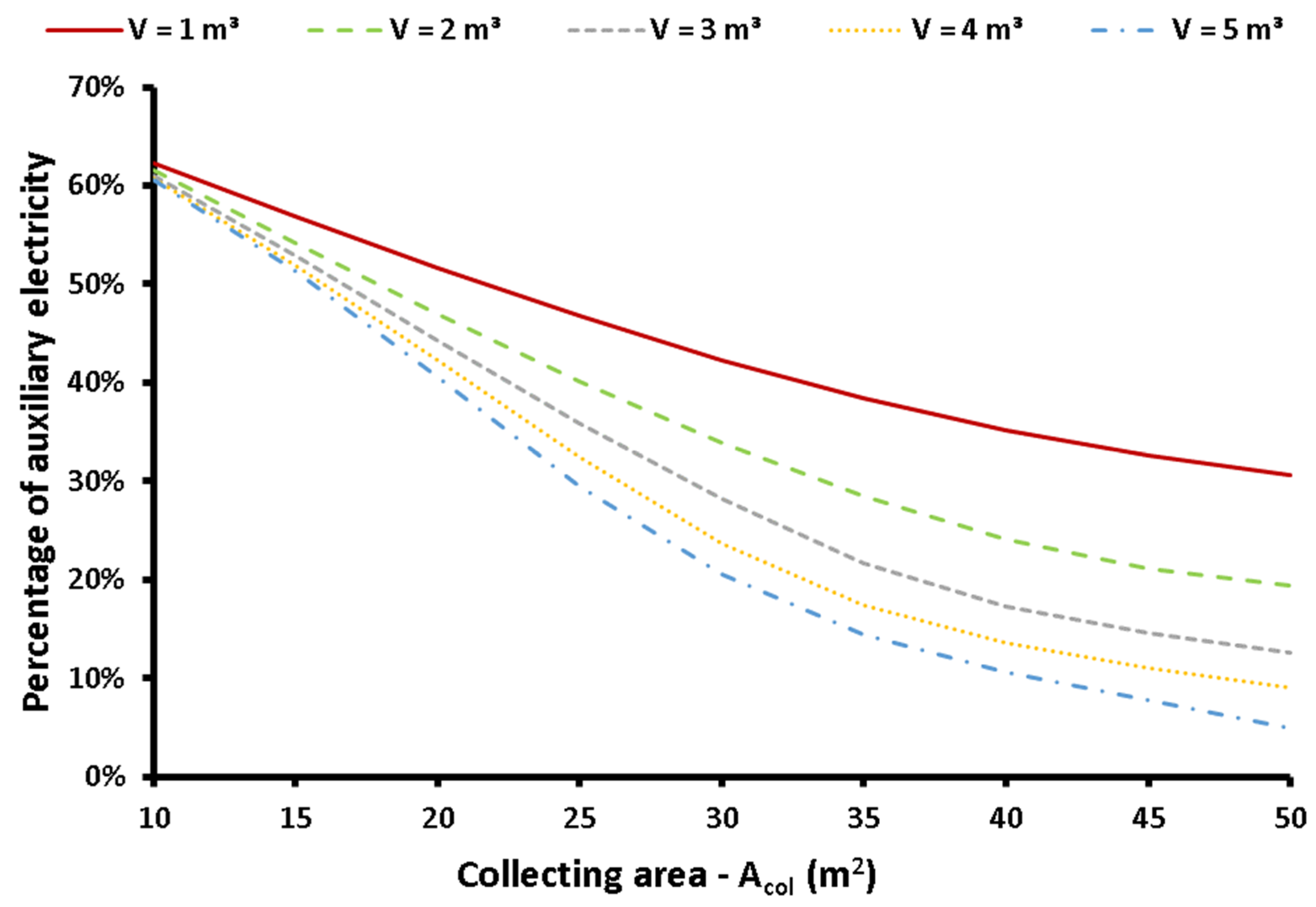
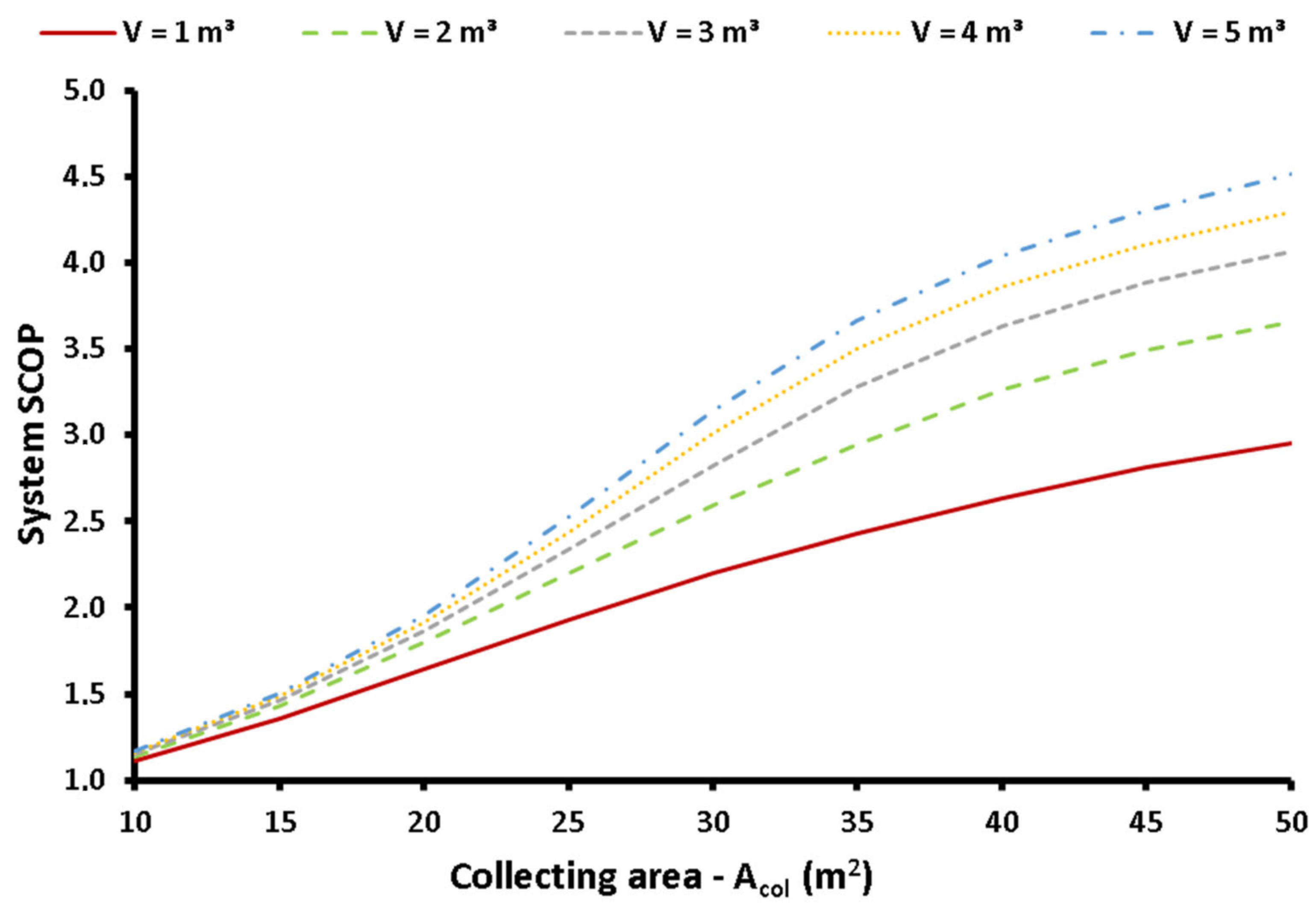
It was found that an increase in the solar field area and of the thermal tank volume leads to higher useful heat produced by the exploitation of the sun and consequently to a greater performance in the system.

-

The auxiliary heater aids the mean tank temperature to be kept at the desired levels and it is activated only for a small time period which is only 6.2% of the heating time.

-

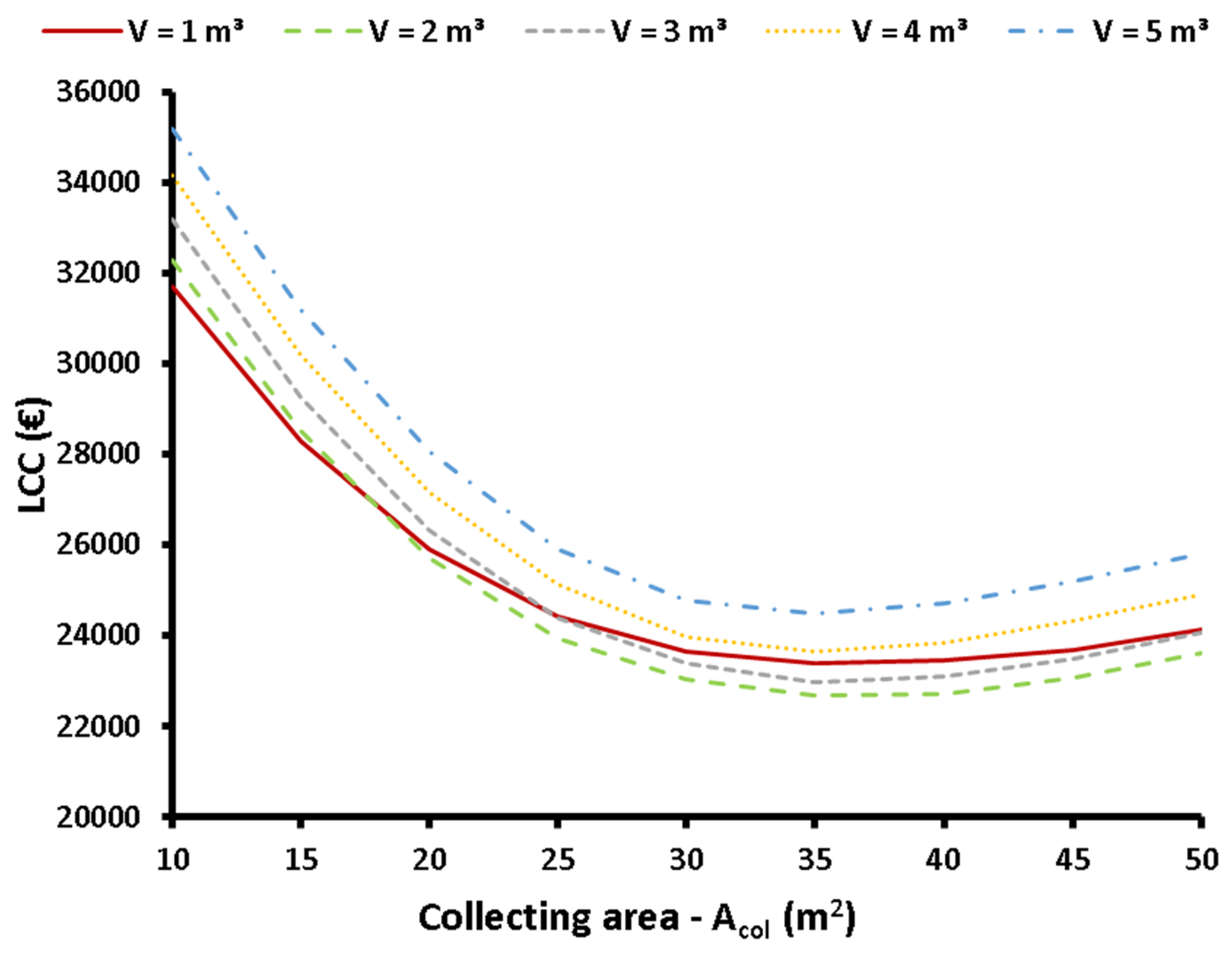
According to the results, the economic optimization indicates that the optimal design includes 35 m² of solar thermal collectors connected to a storage tank of 2 m³ for facing the total heating demand of 6785 kWh. In this case, the life cycle cost was calculated at 22,694 EUR, the seasonal system coefficient of performance at 2.947 and the mean solar thermal efficiency at 31.60%.

-

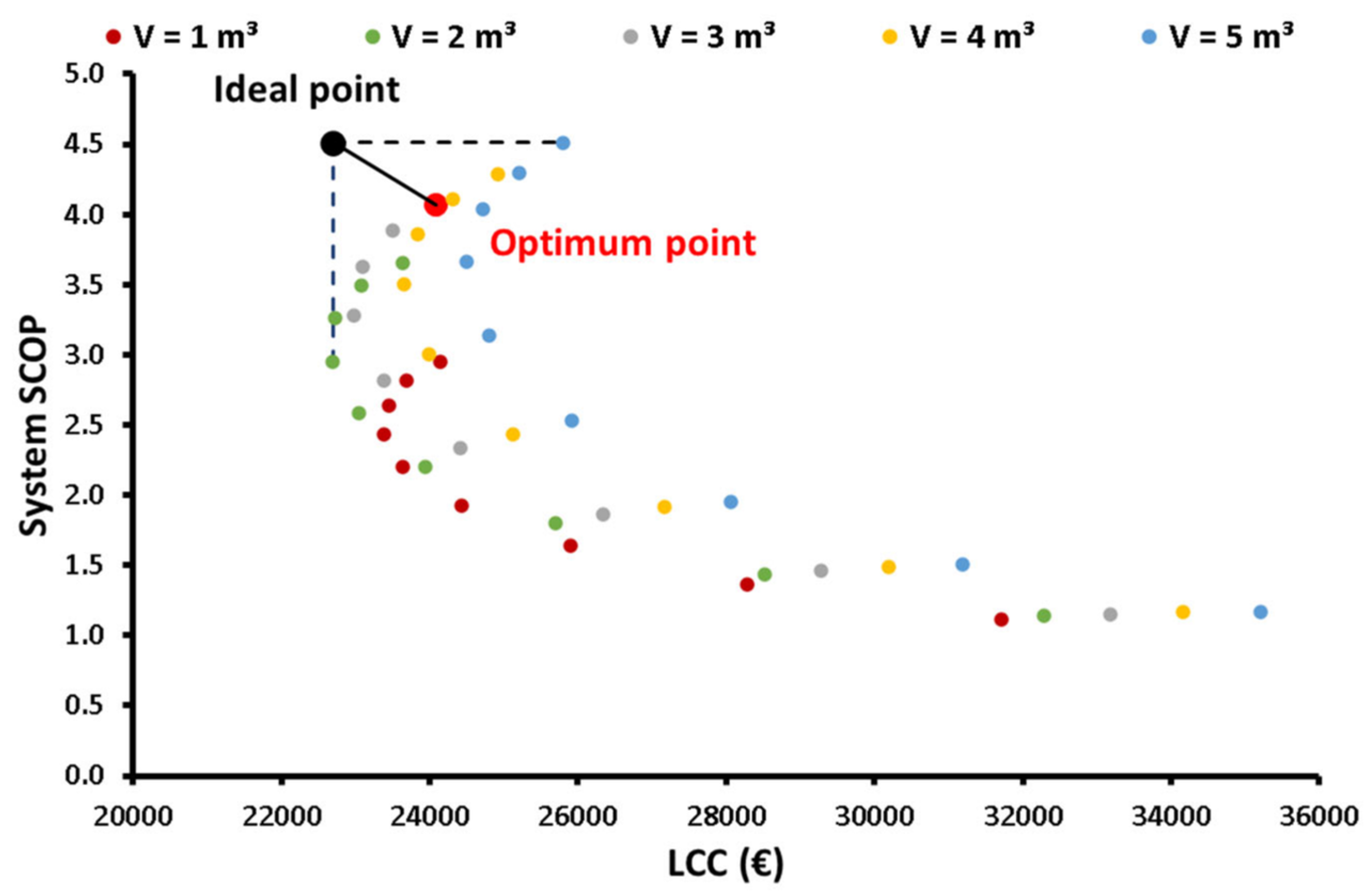
The multi-objective optimization with both energetic and economic criteria indicates that the optimum design is the selection of 50 m² of solar thermal collectors connected to a storage tank of 3 m³. In this case, the life cycle cost was calculated at 24,084 EUR, the seasonal system coefficient of performance at 4.066 and the mean solar thermal efficiency at 25.33%.

-

It can be concluded that the rise in the solar field area leads to significant enhancements to the system performance by leading to electricity savings, while the additional cost is reasonable, according to the life cycle cost analysis.

In the future, it would be interesting to examine a system with both solar and geothermal inputs in a high-temperature heat pump. Moreover, the present system can be examined in other locations with different heating demands and solar potential values. An extra interesting idea is to couple the present heat pump with a thermal photovoltaic collector which can provide both heat input and electricity. Lastly, the optimization of the present system can be extended by also including environmental criteria.

References

1. European Commission. Communication from the Commission to the European Parliament, the Council, the European Economic and Social Committee and the Committee of the Regions a Renovation Wave for Europe—Greening our Buildings, Creating Jobs, Improving Lives; European Commission: Brussels, Belgium, 2020.
2. Hielscher, S.; Wittmayer, J.M.; Dańkowska, A. Social movements in energy transitions: The politics of fossil fuel energy pathways in the United Kingdom, the Netherlands and Poland. Extr. Ind. Soc. 2022, 10, 101073. [Google Scholar] [CrossRef]
3. Chomać-Pierzecka, E.; Kokiel, A.; Rogozińska-Mitrut, J.; Sobczak, A.; Soboń, D.; Stasiak, J. Analysis and Evaluation of the Photovoltaic Market in Poland and the Baltic States. Energies 2022, 15, 669. [Google Scholar] [CrossRef]
4. Wang, Z.; Li, G.; Wang, F.; Zhang, Y. Performance investigation of a transcritical CO2 heat pump combined with the terminal of radiator and floor radiant coil for space heating in different climates, China. J. Build. Eng. 2021, 44, 102927. [Google Scholar] [CrossRef]
5. Jiang, J.; Hu, B.; Wang, R.Z.; Deng, N.; Cao, F.; Wang, C.-C. A review and perspective on industry high-temperature heat pumps. Renew. Sustain. Energy Rev. 2022, 161, 112106. [Google Scholar] [CrossRef]
6. Bellos, E.; Tzivanidis, C. Energetic and financial sustainability of solar assisted heat pump heating systems in Europe. Sustain. Cities Soc. 2017, 33, 70–84. [Google Scholar] [CrossRef]
7. Kong, X.; Yan, X.; Yue, Z.; Zhang, P.; Li, Y. Influence of refrigerant charge and condenser area on direct-expansion solar-assisted heat pump system for radiant floor heating. Sol. Energy 2022, 247, 499–509. [Google Scholar] [CrossRef]
8. Hu, Z.; Gao, Z.; Xu, X.; Fang, S.; Zhou, L.; Ji, D.; Li, F.; Feng, J.; Wang, M. Suitability zoning of buried pipe ground source heat pump and shallow geothermal resource evaluation of Linqu County, Shandong Province, China. Renew. Energy 2022, 198, 1430–1439. [Google Scholar] [CrossRef]
9. Deng, J.; Ma, M.; Wei, Q.; Liu, J.; Zhang, H.; Li, M. A specially-designed test platform and method to study the operation performance of medium-depth geothermal heat pump systems (MD-GHPs) in newly-constructed project. Energy Build. 2022, 272, 112369. [Google Scholar] [CrossRef]
10. Lyakhomskii, A.; Petrochenkov, A.; Romodin, A.; Perfil’eva, E.; Mishurinskikh, S.; Kokorev, A.; Kokorev, A.; Zuev, S. Assessment of the Harmonics Influence on the Power Consumption of an Electric Submersible Pump Installation. Energies 2022, 15, 2409. [Google Scholar] [CrossRef]
11. Souhail, W.; Alsharif, S.; Ahmed, I.; Khammari, H. Optimal Tradeoff between MPP and Stability of a PV-Based Pumping System. Energies 2022, 15, 1106. [Google Scholar] [CrossRef]
12. Nandhini, R.; Sivaprakash, B.; Rajamohan, N. Waste heat recovery at low temperature from heat pumps, power cycles and integrated systems—Review on system performance and environmental perspectives. Sustain. Energy Technol. Assess. 2022, 52, 102214. [Google Scholar] [CrossRef]
13. Li, J.; Qu, C.; Li, C.; Liu, X.; Novakovic, V. Technical and economic performance analysis of large flat plate solar collector coupled air source heat pump heating system. Energy Build. 2022, 277, 112564. [Google Scholar] [CrossRef]
14. Gaonwe, T.P.; Hohne, P.A.; Kusakana, K. Optimal energy management of a solar-assisted heat pump water heating system with a storage system. J. Energy Storage 2022, 56, 105885. [Google Scholar] [CrossRef]
15. Li, J.; Wei, S.; Dong, Y.; Liu, X.; Novakovic, V. Technical and economic performance study on winter heating system of air source heat pump assisted solar evacuated tube water heater. Appl. Therm. Eng. 2023, 221, 119851. [Google Scholar] [CrossRef]
16. Jiang, Y.; Zhang, H.; Wang, Y.; Wang, Y.; Liu, M.; You, S.; Wu, Z.; Fan, M.; Wei, S. Research on the operation strategies of the solar assisted heat pump with triangular solar air collector. Energy 2022, 246, 123398. [Google Scholar] [CrossRef]
17. Leonforte, F.; Miglioli, A.; Del Pero, C.; Aste, N.; Cristiani, N.; Croci, L.; Besagni, G. Design and performance monitoring of a novel photovoltaic-thermal solar-assisted heat pump system for residential applications. Appl. Therm. Eng. 2022, 210, 118304. [Google Scholar] [CrossRef]
18. Yang, L.W.; Xu, R.J.; Zhou, W.B.; Li, Y.; Yang, T.; Wang, H.S. Investigation of solar assisted air source heat pump heating system integrating compound parabolic concentrator-capillary tube solar collectors. Energy Convers. Manag. 2023, 277, 116607. [Google Scholar] [CrossRef]
19. Bellos, E.; Tzivanidis, C.; Moschos, K.; Antonopoulos, K.A. Energetic and financial evaluation of solar assisted heat pump space heating systems. Energy Convers. Manag. 2016, 120, 306–319. [Google Scholar] [CrossRef]
20. Plytaria, M.T.; Bellos, E.; Tzivanidis, C.; Antonopoulos, K.A. Financial and energetic evaluation of solar-assisted heat pump underfloor heating systems with phase change materials. Appl. Therm. Eng. 2019, 149, 548–564. [Google Scholar] [CrossRef]
21. Bellos, E.; Tzivanidis, C.; Nikolaou, N. Investigation and optimization of a solar assisted heat pump driven by nanofluid-based hybrid PV. Energy Convers. Manag. 2019, 198, 111831. [Google Scholar] [CrossRef]
22. Welcome TRNSYS: Transient System Simulation Tool. Available online: https://www.trnsys.com/ (accessed on 17 December 2022).
23. EES: Engineering Equation Solver F-Chart Software: Engineering Software. Available online: https://fchartsoftware.com/ees/ (accessed on 17 December 2022).
24. Mota-Babiloni, A.; Navarro-Esbrí, J.; Molés, F.; Cervera, Á.B.; Peris, B.; Verdú, G. A review of refrigerant R1234ze(E) recent investigations. Appl. Therm. Eng. 2016, 95, 211–222. [Google Scholar] [CrossRef]
25. Bellos, E.; Tzivanidis, C.; Belessiotis, V. Daily performance of parabolic trough solar collectors. Sol. Energy 2017, 158, 663–678. [Google Scholar] [CrossRef]
26. Welcome to BITZER. Available online: https://www.bitzer.de/gr/en/ (accessed on 17 December 2022).
27. BITZER Software. Available online: https://www.bitzer.de/websoftware/Default.aspx (accessed on 17 December 2022).
28. Available online: http://portal.tee.gr/portal/page/portal/SCIENTIFIC_WORK/GR_ENERGEIAS/kenak/files/TOTEE_20701-1_2017_TEE_1st_Edition.pdf (accessed on 17 December 2022).
29. ISO 7730:2005. Available online: https://www.iso.org/standard/39155.html (accessed on 17 December 2022).
30. Solar Collector Calpak M4. Available online: https://calpak.gr/el/products/iliakoi-sullektes-boilers/33/210 (accessed on 6 January 2023).
31. Solar Engineering of Thermal Processes, 4th Edition Wiley. Available online: https://www.wiley.com/en-us/Solar+Engineering+of+Thermal+Processes%2C+4th+Edition-p-9780470873663 (accessed on 6 January 2023).
32. Bellos, E.; Tzivanidis, C.; Antonopoulos, K.A. Exergetic, energetic and financial evaluation of a solar driven absorption cooling system with various collector types. Appl. Therm. Eng. 2016, 102, 749–759. [Google Scholar] [CrossRef]
33. Bellos, E.; Tsimpoukis, D.; Lykas, P.; Kitsopoulou, A.; Korres, D.N.; Vrachopoulos, M.G.; Tzivanidis, C. Investigation of a High-Temperature Heat Pump for Heating Purposes. Appl. Sci. 2023, 13, 2072. [Google Scholar] [CrossRef]
34. Bellos, E.; Tzivanidis, C.; Symeou, C.; Antonopoulos, K.A. Energetic, exergetic and financial evaluation of a solar driven absorption chiller—A dynamic approach. Energy Convers. Manag. 2017, 137, 34–48. [Google Scholar] [CrossRef]
35. Heat Pumps YDOR. Available online: https://www.ydor.com.gr/antlies-thermotitas/?gclid=CjwKCAiAp7GcBhA0EiwA9U0mtkyRiiUfH5m8RsWav7hpm85YOuhnNqXMx851rw63fKlo_KWaUNVcxRoCgzwQAvD_BwE&f2--=6-kw&page=2 (accessed on 17 December 2022).
36. Bellos, E.; Sarakatsanis, I.; Tzivanidis, C. Investigation of Different Storage Systems for Solar-Driven Organic Rankine Cycle. Appl. Syst. Innov. 2020, 3, 52. [Google Scholar] [CrossRef]
Figure 1. The examined system with a solar-assisted heating unit which includes a solar field, a thermal storage tank with auxiliary electrical resistance and a high-temperature heat pump.
Applsci 13 04066 g001
Figure 2. Performance of the heat pump for different operating conditions.
Applsci 13 04066 g002
Figure 3. Depiction for the accuracy of the approximation formula for the heat pump COP.
Applsci 13 04066 g003
Figure 4. Climate conditions of Athens in the winter period (1 October to 30 April).
Applsci 13 04066 g004
Figure 5. Heating load and cumulative heating demand for the examined building (1 October to 30 April).
Applsci 13 04066 g005
Figure 6. Mean water temperature in the storage tank for the case with 30 m2 collecting area and 3 m3 tank volume (1 October to 30 April).
Applsci 13 04066 g006
Figure 7. Electricity demand for the compressor and the auxiliary electrical resistance in the tank for the case with 30 m2 collecting area and 3 m3 tank volume (1 October to 30 April).
Applsci 13 04066 g007
Figure 8. COP for the system and the heat pump for the case with a 30 m2 collecting area and 3 m3 tank volume (1 October to 30 April).
Applsci 13 04066 g008
Figure 9. Variation in energy quantities for different collecting areas with the storage tank volume at 3 m3.
Applsci 13 04066 g009
Figure 10. Variation in energy quantities for different storage tank volumes with the collecting area at 30 m2.
Applsci 13 04066 g010
Figure 11. Mean yearly solar thermal efficiency of the collectors for different combinations of (Acol) and (V).
Applsci 13 04066 g011
Figure 12. Total electricity demand (compressor and auxiliary electrical resistance) for different combinations of (Acol) and (V).
Applsci 13 04066 g012
Figure 13. Percentage of the auxiliary electricity compared to the total electricity demand for different combinations of (Acol) and (V).
Applsci 13 04066 g013
Figure 14. System seasonal COP for different combinations of (Acol) and (V).
Applsci 13 04066 g014
Figure 15. Life cycle cost of the heating system for different combinations of (Acol) and (V).
Applsci 13 04066 g015
Figure 16. Illustration of the multi-objective optimization process of the system aiming for the maximization of the system SCOP and the minimization of the LCC.
Applsci 13 04066 g016