Atmospheric Density Inversion Based on Swarm-C Satellite Accelerometer

Abstract

We used the Swarm-C accelerometer data to invert the orbital atmospheric density in this study. First, the Swarm-C satellite mission data were obtained from the ESA’s public data platform, and preliminary data error correction was performed. This paper refers to the calibration method of GRACE-A satellite accelerometer data. It adds linear temperature correction on the original basis. Moreover, this study’s accelerometer data correction results were compared with the data correction results published by the ESA. In order to explore the influence of light radiation on the accelerometer, we established a geometric model of Swarm-C to simulate the physical shape of the satellite surface. The light radiation pressure model and the shadow area judgment model were established, the change in the light radiation acceleration during the transition process of the satellite from the umbra area to the penumbra area and then to the shadowless area was studied, and the state transition during the transition process was analyzed. Finally, the atmospheric drag coefficient was calculated based on the Sentman model. Atmospheric density inversion calculations were performed using the above data. We show the spatial distribution of atmospheric density at a fixed latitude, testing our results during geomagnetic storms. We compared the density results with existing research data, demonstrating the effectiveness of our approach.

1. Introduction

Research on thermospheric density has significant meaning for different applications and satellite orbits. Its application scope includes satellite re-entry prediction, maneuver planning and space object orbit maintenance, and propellant fuel carrying capacity estimation. The drag resistance of the atmosphere is the essential component of the non-conservative forces of low-orbit satellites. Therefore, the measurement accuracy of atmospheric density largely determines the satellite’s non-conservative force [1]. However, it is challenging to measure and forecast atmospheric density. The empirical atmospheric model’s prediction accuracy is affected by the Earth’s magnetic field change, solar activity cycle, and Earth’s rotation [2,3,4]. As a result, the empirical atmospheric density model’s prediction accuracy is limited. Satellite manipulation and orbit determination require high-precision information on thermosphere atmospheric density [1,5,6]. Hence, studying the complex characteristics of the thermosphere and satellite dynamics modeling is challenging.

It is of great significance to study the density of the thermosphere. Under the influence of the complex interaction between the Earth’s system and the Sun, the thermosphere atmospheric density has a wide range of spatiotemporal variations [7,8]. However, the observed data on thermosphere atmospheric density have been very scarce, so the modeling uncertainty of thermosphere atmospheric density is very high [9].

There are three main methods for detecting the thermosphere’s density. The first is to use atmospheric density detectors [10]. The mechanism is based on aerodynamics by detecting the temperature inside the sensor and the pressure of the vessel wall. This method is traditional and needs more time. It cannot reflect the atmospheric density around the spacecraft’s orbit in time and has low accuracy. The second method is to use orbit data inversion. It is a primary method for thermospheric density measuring. Many known semi-empirical atmospheric models are built upon this method [4,11,12,13]. The method’s basic principle is that the atmospheric resistance causes all LEO (low Earth orbit) space objects to spiral downward and eventually re-enter the densest atmosphere. Since the atmospheric density decreases exponentially as the height increases, the elliptical orbit object is subjected to the most potent resistance at its perigee. The resistance causes the kinetic energy to be converted into heat orbital size, reducing the space object’s ellipticity [14]. When the space object approaches the end of its life, its orbit becomes almost circular. The density and resistance along the orbit rapidly increase. The long axis decays rapidly, and the decay rate can reach 30 km daily. The satellite deviates from the predetermined orbit under atmospheric drag, so the relationship between the change of the orbital parameters and the atmospheric density can reverse the atmospheric density. The third method uses an onboard accelerometer [15,16,17]. The accuracy of the onboard accelerometer is very high, and the gravity satellites CHAMP, GRACE, and Swarm satellites are all equipped with this kind of load.

Since the 1960s, satellites from the United States, Italy, and France have carried onboard accelerometers for the study of thermospheric airtight modeling. Beginning in 1968, miniature electrostatic uniaxial accelerometers (MESA) were applied to eight satellites in orbit. Italy launched the spherical San Marco satellite in 1968, carrying an accelerometer. France launched the CASTOR satellite carrying the CACTUS accelerometer in 1975. ONERA developed the CACTUS accelerometer. The satellite was mainly used to test the operation of the CACTUS accelerometer. As an improvement of MESA, the satellite electrostatic three-axis accelerometer (SETA) was used in multiple space missions of the U.S. military for testing in the first half of the 1980s.

Some scholars and institutions have used satellite accelerometer data to detect atmospheric density. At first, French space agency researchers used CHAMP’s accelerometer data to retrieve the atmospheric density. The accuracies of the DTM (Drag Temperature Model) series and the MSIS (Multiple Sclerosis Impact Scale) series were evaluated using the inversion results. The DTM–STAR model was obtained after improving the DTM-2000 model [18]. Sutton and other scholars used the CHAMP satellite’s accelerometer data to study the atmospheric density from October to November 2003. They also studied atmospheric density distribution differences between the northern and southern hemispheres. Using the inversion results, they evaluated the MSIS00 atmospheric model’s accuracy and HWM93 (Horizontal Wind Model 93) [12,19]. RW Zurek et al. used the MAVEN spacecraft’s accelerometer data to detect the upper atmosphere’s structure on Mars, estimated the vertical distribution of Martian atmospheric temperature, and reconstructed the profile to 170 km [17]. Doornbos et al. proposed an iterative algorithm for measuring atmospheric density and wind field using satellite accelerometer data [20]. Emmert et al. calculated the mean error between the measured results and the empirical model [21]. PM Mehta et al. obtained the latest atmospheric density data set by re-scaling Sutton’s mass density datasets of CHAMP and GRACE satellites [22]. Pieter Visser et al. used TDW (Thermospheric density and wind), and Ghost software provided by NASA to retrieve the thermosphere and horizontal wind fields of the GRACE and CHAMP satellites. They analyzed the feasibility of retrieving atmospheric density from the accelerometer data Swarm satellite. Unfortunately, the author did not conduct specific experiments and research on Swarm satellites [23]. Densities from accelerometers on Swarm-C were retrieved by Siemes et al. [24].

The main points of this paper are as follows: the Swarm-C accelerometer data were corrected by referring to the correction method of the GRACE-A satellite accelerometer [25,26]. The correction results were compared with the data correction results published by ESA (https://earth.esa.int/eogateway/missions/swarm/data) (accessed on 18 November 2022). Then, the satellite surface shape model was established, and the simplified conical shadow model replaced the traditional cylindrical shadow model for light radiation pressure modeling [27,28]. The similarities and differences between the modeling effects of the two models were compared. Finally, the atmospheric drag coefficient of the Swarm-C satellite was calculated [29,30], and the atmospheric density was retrieved.

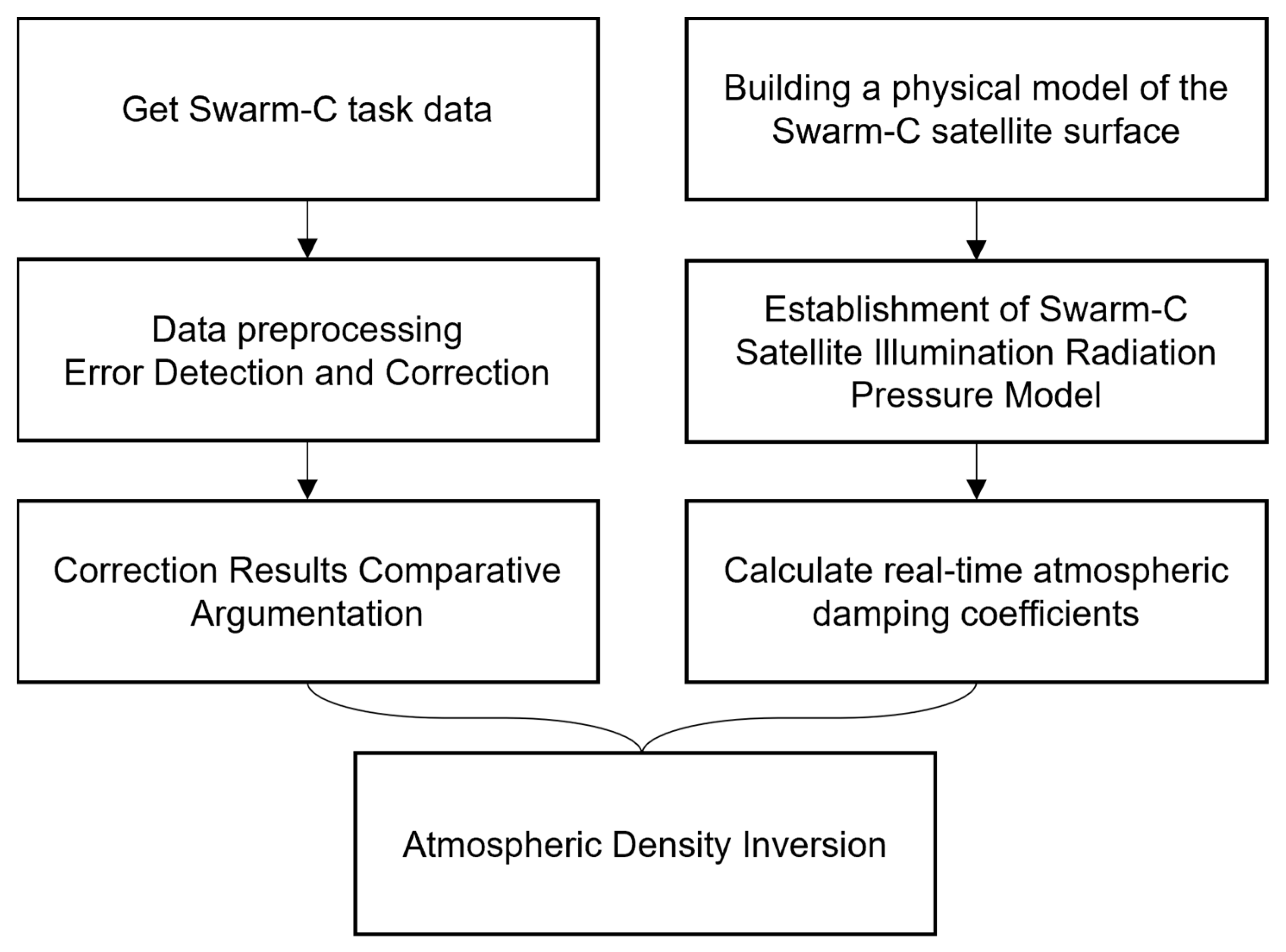
2. Materials and Methods

The main workflow of this study is shown in Figure 1.

2.1. Data Preprocessing and Correction

For the Swarm-C satellite, although ESA will publish the accelerometer data of the satellite every once in a while, due to the delay in the data being published by the ESA, the data published by the ESA remained in 2016, when this study was carried out. As a result, ESA only published the corrected results among the three Swarm satellites [31]. Since the accelerometer data of the Swarm-C satellite after 2017 need to be used in this paper, we try to refer to the correction method of the GRACE-A satellite [25] to correct the original accelerometer data of the Swarm-C satellite. We obtained Swarm-C accelerometer data from ESA’s public data platform (http://swarm-diss.eo.esa.int/) (accessed on 18 November 2022). These include uncalibrated raw accelerometer data and non-conservative force acceleration data derived from GPS [32].

There is a detailed description of Swarm satellite data in the link (https://earth.esa.int/eogateway/documents/20142/37627/Swarm-PDGS-Data-Access-User-Manual.pdf) (accessed on 18 November 2022).

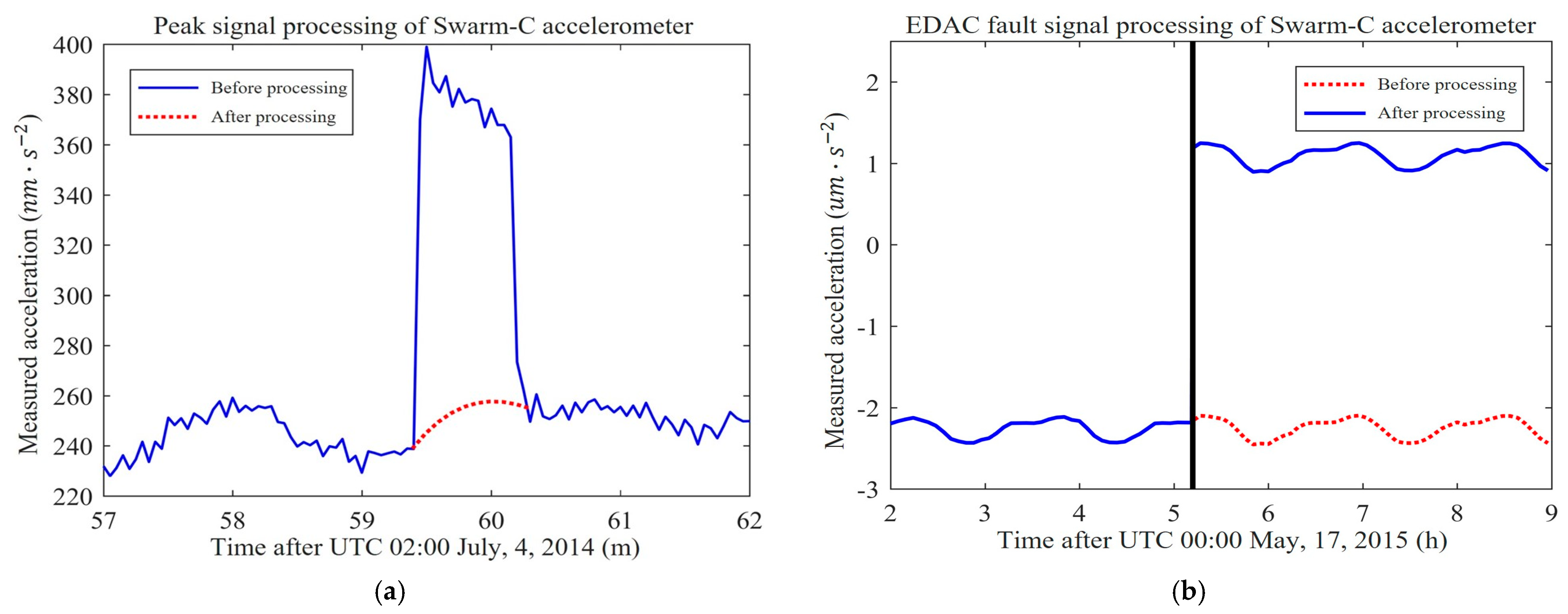
2.1.1. Preprocessing of Swarm-C Accelerometer Data

This step processes the spike signal caused by the propellant and the data anomaly caused by the error detection and correction (EDAC) fault event in the accelerometer data. These two data anomalies are also unique to the Swarm-C satellite. Errors in the accelerometer’s RAM code memory occur approximately once a month and per satellite. The error usually occurs in the South Atlantic Anomaly and polar regions. The cause of the malfunction may have originated from cosmic radiation. Since the EDAC implementation sometimes fails, the easiest way to recover from the error is to restart the accelerometer, i.e., turn the instrument off and on again.

During the operation of the Swarm-C satellite in orbit, when the control torque from magnetic torque is not enough to maintain the satellite’s attitude, the attitude propellant will be activated. Since the thrusters have a short start-up time and are of the switch (Boolean) type, they produce a transient acceleration peak lasting for several seconds that can be detected by the accelerometer, which produces an acceleration spike signal. Although the accelerometer will record the acceleration spike signal caused by the propellant, this part of the data needs to be eliminated when calculating the aerodynamic acceleration. The resulting data gap needs to be filled by interpolation. The accelerometer spike signal caused by the propellant and the processed results are shown in Figure 2a.

In the accelerometer data of the Swarm-C satellite, the accelerometer data abnormality caused by the EDAC fault event also needs preprocessing. For example, Figure 2b records an EDAC failure event of the Swarm-C satellite on 17 May 2015. The curve of accelerometer data shows a massive step after experiencing the EDAC failure event. The blue signal represents the data before correction, and the red curve represents the accelerometer data after correction.

In case of an EDAC fault event during accelerometer data processing of the Swarm-C satellite, manual displacement correction can be performed on the step signal in the data.

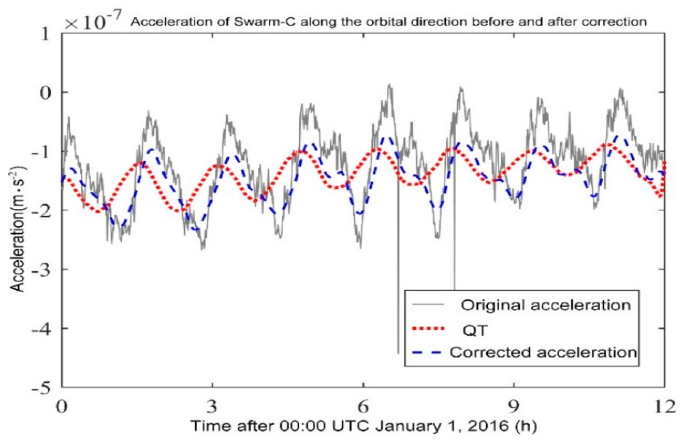
2.1.2. Data Correction Method of Swarm-C Accelerometer

This study will refer to the GRACE-A satellite accelerometer’s calibration method when calibrating the Swarm-C satellite’s accelerometer [25,26,33,34,35]. Slightly different from previous research, the main content of Swarm-C accelerometer correction is the data error caused by the temperature change of the accelerometer carrier. Given this feature, this section will add a linear temperature correction and compare the final correction results with ESA’s.

For each point of the satellite orbit, the calibration equation is defined as shown in Equation (1) [25,26], where $a_{ACC}^{UNCAL}$ represents the uncalibrated accelerometer data, $Q$ represents a linear temperature factor, $T\left(t+F\right)$ represents a temperature signal with a time shift of $F$, $B$ represents the coefficient of deviation, $S$ represents the scale coefficient, $G$ represents the trend coefficient, $t$ and $t_0$ represent the elapsed time and the start time, respectively, and $\epsilon$ represents noise.

$$a_{NG}^{GPS}=B+S\cdot a_{ACC}^{UNCAL}+Q\cdot T\left(t+F\right)+G\cdot \left(t-t_0\right)+\epsilon$$

(1)

In this paper, the non-conservative force acceleration data derived from GPS are used as the calibration standard, which is projected in the direction of the calibrated accelerometer data component to obtain the projected non-conservative acceleration $a_{NG}^{GPS}$. Then, combined with Equation (1) to find the calibration parameters $\widehat{B}$, $\widehat{S}$, $\widehat{Q}$, $\widehat{G}$, through the generalized least square method, the estimated value of the linear calibration parameters is expressed by adding a pointed cap to the variable. After obtaining the estimated value of the variable, the corrected acceleration value $a_{ACC}^{CAL}$ can be calculated by Equation (2). Figure 3 compares the accelerometer data of the Swarm-C satellite before and after correction.

$$a_{ACC}^{CAL}=\widehat{B}+\widehat{S}\cdot a_{ACC}^{UNCAL}+\widehat{Q}\cdot T\left(t+F\right)+\widehat{G}\cdot \left(t-t_0\right)$$

(2)

As shown in Figure 3, the gray curve is the original accelerometer signal. After correcting the method in this paper, the accelerometer data becomes smooth, as shown by the blue curve. The red curve is the $\widehat{Q}\cdot T$ temperature term in Equation (2). The figure shows the influence of the temperature term on acceleration. The amplitude of the temperature term accounts for more than 50% of the amplitude of the corrected data curve. It proves that the accelerometer data error caused by temperature is relatively large for Swarm-C satellites. Therefore, it is necessary to perform linear temperature correction on the accelerometer data.

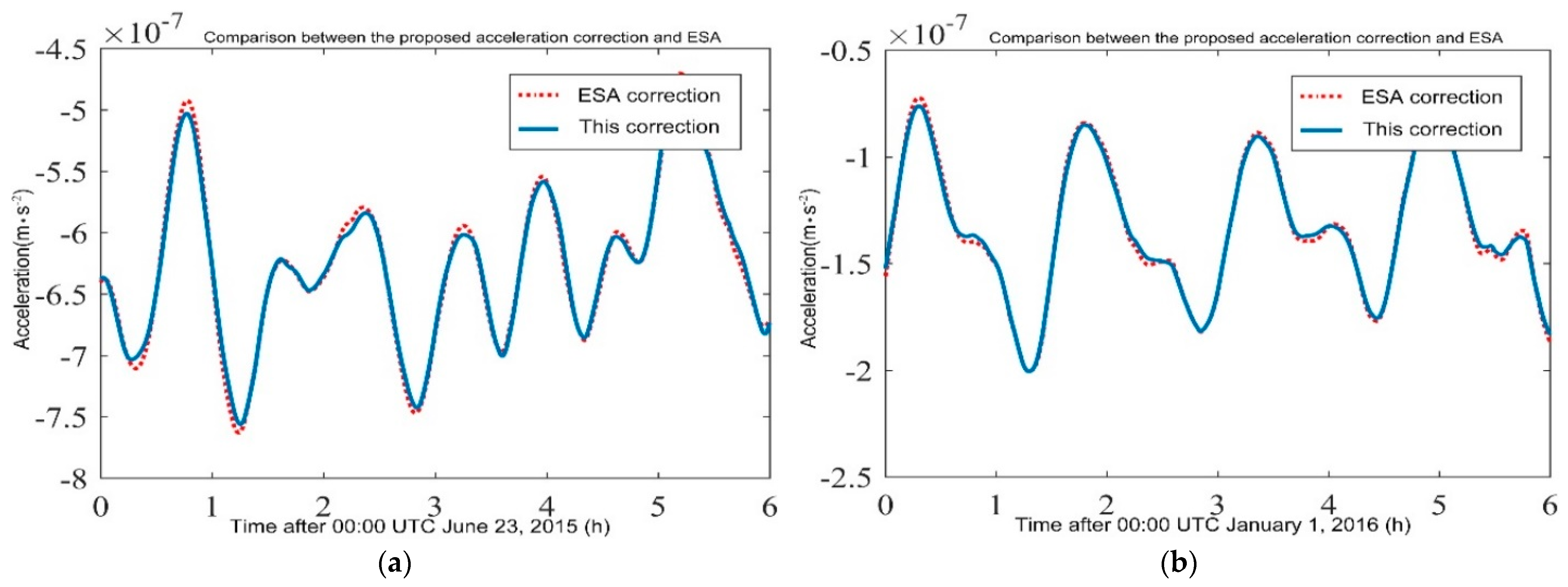
2.1.3. Comparison of Calibration Results

This article calibrates and discusses only the acceleration data along the satellite orbit direction. The acceleration data in other directions can be performed in the same way.

The comparison between the results from the improved correction method and the ESA correction is shown in Figure 4. Among them, Figure 4a is the result of the correction by the magnetic storm day accelerometer data. Figure 4b is the correction result of a nonmagnetic storm day.

Figure 4a shows the accelerometer data during a strong magnetic storm with a level of G4, and Figure 4b shows the accelerometer data during a normal period. It can be seen that the fluctuation frequency of the accelerometer increases significantly during the strong magnetic storm occurrence period. The reason for the above phenomenon is that the magnetic pressure will cause a huge change in the particle density of the atmosphere.

As seen in Figure 4, the accelerometer data correction results obtained using the improved correction method in this paper are very close to the accelerometer correction results published by ESA. Therefore, the coincidence between the two is very high, which shows the accuracy of the correction method in this paper.

2.2. Method and Model

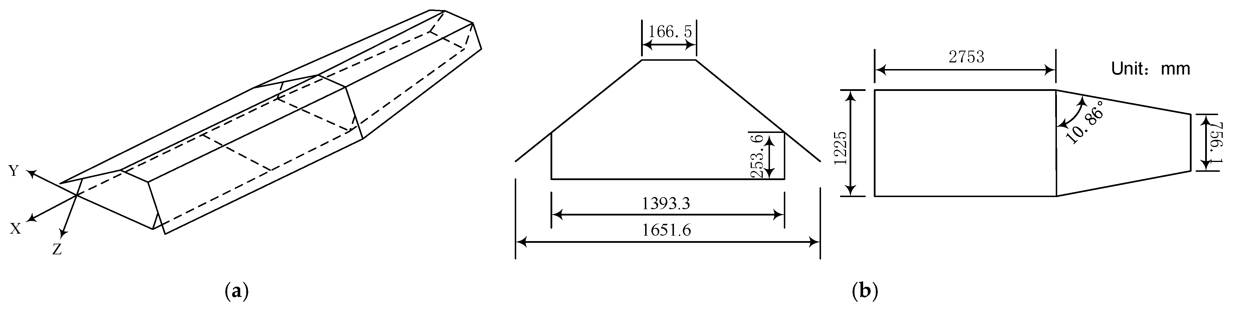
2.2.1. Swarm-C Satellite Surface Model

The coordinate system of each normal panel vector is the star-fixed coordinate system of the SWARM-C satellite. The star-fixed coordinate system is centered on the satellite’s center of mass, and the three coordinate axes, X, Y, and Z, form a right-handed coordinate system. In this paper’s calculation, the illumination radiation pressure modeling needs to use the attitude data of the space-borne camera to realize the conversion between the star-fixed coordinate system and the inertial coordinate system.

In Swarm’s manual, ESA provides each panel’s size and optical characteristic parameters. Therefore, compared with GRACE, Swarm’s panel composition is more complex. For example, the Swarm-C satellite contains 15 panels in total. Figure 5a shows the simplified shape diagram of the Swarm-C satellite. Figure 5b shows the Swarm-C satellite’s side panel and bottom panel schematic diagram.

Taking the motion direction as the x-axis, the normal vector of each panel of the Swarm-C satellite can be calculated.

Table 1. Normal vectors of each panel of Swarm-C satellite.

Panel	Area	X	Y	Z
Nadir 1	1.540	0.0	0.0	1.0
Nadir 2	1.400	−0.19766	0.0	0.98027
Nadir 3	1.600	−0.13808	0.0	0.99042
Solar Array +Y	3.450	0.0	0.58779	−0.80902
Solar Array −Y	3.450	0.0	−0.58779	−0.80902
Zenith	0.500	0.0	0.0	−1.0
Front	0.560	1.0	0.0	0.0
Side Wall +Y	0.753	0.0	1.0	0.0
Side Wall −Y	0.753	0.0	−1.0	0.0
Shear Panel Nadir Front	0.800	1.0	0.0	0.0
Shear Panel Nadir Back	0.800	−1.0	0.0	0.0
Boom +Y	0.600	0.0	1.0	0.0
Boom −Y	0.600	0.0	−1.0	0.0
Boom Zenith	0.600	−0.23924	0.0	−0.97096
Boom Nadir	0.600	0.22765	0.0	0.97374

shows the normal vectors of each panel of the Swarm-C satellite.

Because there are many panels of the Swarm-C satellite, and some panels are not perpendicular to the coordinate axis, it will be much more challenging to model the surface of the Swarm-C satellite and judge the shadow area.

2.2.2. Swarm-C Satellite Cone Shadow Modeling

A cylindrical shadow model is used in the existing satellite shadow area modeling [27]. Both the Sun and the Earth are regarded as circular spheres. The Sun’s rays are considered to be parallel to the line between the center of the Sun and the center of the Earth’s sphere, with the Earth blocking the Sun’s rays to create a cylindrical shadow area. However, the radius of the Sun is 109 times that of the Earth. Therefore, the Sun’s rays are non-parallel, so the shadow area of the cylindrical model can be further divided into the main shadow area, penumbra area, and artifact area. However, because the artifact area is very far from the Earth’s center, the LEO satellites studied in this paper will not involve this area. Therefore, the shadow can be divided into penumbra and umbra to simplify the original cone shadow model.

The difficulty in building the simplified conical shadow model lies in the treatment of the transition zone of the satellite from principal shadow to penumbra to full-shadowed or from full-shadowed to penumbra to principal shadow. The simplified conical shadow model shown in Figure 6 does not consider the refraction of the atmosphere and assumes that the solar illumination is smoothly varying. After applying the simplified conical shadow model with the Earth occluding the Swarm-C satellite for the experiment, the acceleration caused by the light radiation pressure along the orbital direction, the cross-orbit direction, and the radial direction, when the Swarm-C satellite leaves the penumbra region and enters the penumbra region can be calculated [27,28]. In the simulated orbit, the light radiation pressure acceleration in three directions is shown in Figure 7.

It can be seen from Figure 7 that the satellite is completely covered from about 0–20 s. The satellite’s along-track direction, cross-track direction, and radial radiation pressure acceleration are all 0, and the satellite is in the umbra area at this time. From 20 s to 40 s, the satellite gradually leaves the state of complete shading and enters the state of partial illumination. At this time, the acceleration curve changes, and there is a positive or negative light radiation acceleration, and the satellite is in the penumbra. With the gradual decrease of the occulted area of the solar disk and the continuous increase of the shadow coefficient of the penumbra, the absolute value of the pressure acceleration of the light radiation received by satellite is also increasing. This process lasts for about 40 s. After 80 s in the figure, the satellite ultimately enters the illuminated area, that is, the shadowless area. At this time, the pressure velocity of the illuminated radiation received by the satellite reaches an almost constant value.

The satellite’s cross-track direction has the largest change in light radiation pressure for the three directions. In contrast, the satellite’s along-track and radial directions are relatively close to the change. Therefore, when the satellite enters the fully irradiated area, the value of the light radiation acceleration fluctuates little. However, it is still not a completely fixed value because, as the satellite’s flight attitude changes, the effective area exposed to light will also have small changes, so the light radiation acceleration of the satellite will also have small fluctuations. Since the Antumbra area is very far from the Earth’s center, the low-orbit satellites studied in this paper will not reach this area. The shadow can be divided into Umbra and Penumbra areas to simplify the original cone shadow model.

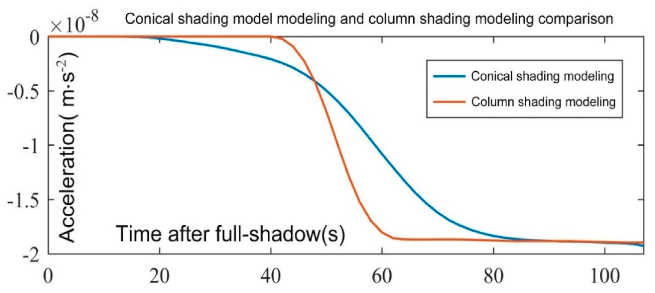
2.2.3. Comparison of Swarm-C Cone Shadow and Column Shadow Modeling

In order to evaluate the effect of the simplified conical shadow model and ensure the accuracy of the satellite surface light radiation pressure modeling, the satellite light radiation pressure acceleration along the orbital direction through the penumbra in the conical shadow model is modeled using the column shadow model. Then, the modeling results are compared using the simplified conical shadow model. The results obtained by modeling the satellite along the orbital direction using the cone-shadow model and the column-shadow model are shown in Figure 8.

As can be seen from Figure 8, the transition time from the full-shadow region to the shadow-free region is longer for the simplified cone-shadow model than for the column-shadow model. In the simplified conical shadow model, the Swarm-C satellite is in the full-shadow region during the 0–20 s, the Swarm-C satellite is in the penumbra region during 20–80 s, and the Swarm-C satellite enters the no-shadow region after the 80 s. Moreover, in the column shadow model, the Swarm-C satellite is in the full-shadow region during 0–42 s. After 62 s, the Swarm-C satellite enters the no-shadow region. For modeling the satellite surface light radiation pressure in the full-shadow and shadowless regions, the difference between the improved cone-shadow model and the column-shadow model is not significant. However, because the Sun’s rays are parallel rays in the column-shadow model, the model does not have the penumbra region, so the transition time of the Swarm-C satellite from the present shadow region to the shadowless region only lasts for about 20 s. In contrast, the transition time of the Swarm-C satellite from the penumbra to the no-shadow region in the conical shadow model lasts about 60 s.

2.2.4. Accelerometer Atmospheric Density Inversion

There are many difficulties in the accurate modeling of atmospheric reverse drag. Since the surface shapes of the Swarm-C satellite and GRACE-A satellite are non-spherical, it is necessary to consider the satellite’s attitude changes during flight and the interaction between gas particles on the satellite surface [25,26].

In atmospheric density calculation, the determination of ballistic coefficient $B$ is very important, and its calculation method is shown in Formula (3) [36], where $C_D$ is the drag coefficient of the satellite, $A$ is the effective area of the satellite, and $m$ is the satellite’s mass.

$$B=\frac{C_{D}A}{m}$$

(3)

The atmospheric drag coefficient $C_D$ and the effective area $A$ of the satellite constantly change with the satellite’s movement. $C_D$ is related to the satellite flight’s attitude and to the physical properties of the materials on the satellite surface and the atmospheric composition state around the satellite orbit; therefore, it is difficult to determine. The atmospheric drag coefficient is calculated by the Sentman model [30,36]. The calculation process will not be repeated.

For the $k$-th panel of the satellite, the product formula of the atmospheric drag coefficient and the effective area of the panel are shown in Equation (4), where ${\gamma }_k$ represents the angle between the normal vector of the k-panel and the incident atmospheric molecules, $A_k$ represents the area of the panel, $C_{D_k}$ is the drag coefficient of the panel, ${\overrightarrow{v}}_r$ represents the velocity of k-panel at location r, and ${\overrightarrow{v}}_{out}$.represents the gas particle’s velocity after collision.

$$C_{D_k}\cdot A_k=(\frac{P}{\sqrt{\pi }}+{\gamma }_{k}QZ+\frac{\gamma }{2}\frac{{\overrightarrow{v}}_{out}}{{\overrightarrow{v}}_r}({\gamma }_k\sqrt{\pi }Z+P))\cdot A_k$$

(4)

In Equation (4), the incident atmospheric molecules are recorded as ${\gamma }_k$, $P=\frac{1}{\left(S\cdot \mathit{exp}(-{\gamma }_k{}^2{S}^2\right))}$, $Q=1+\frac{1}{2S^2}$, $Z=1+\left(\frac{2}{\sqrt{\pi }}\right){\int }_0^{{\gamma }_{k}S}{e}^{-t^2}dt$, where S represents the scale of molecular velocity.

The product of the effective area of the drag coefficient of all satellite panels is added to obtain the result of the overall drag coefficient and the product of the effective area of the satellite. The final atmospheric density $\rho$ around the satellite orbit can be calculated using Equation (5), where $a$ represents the drag acceleration.

$$\rho =\frac{a}{\left(\frac{1}{2}B|{\overrightarrow{v}}_r{|}^2\right)}$$

(5)

3. Results

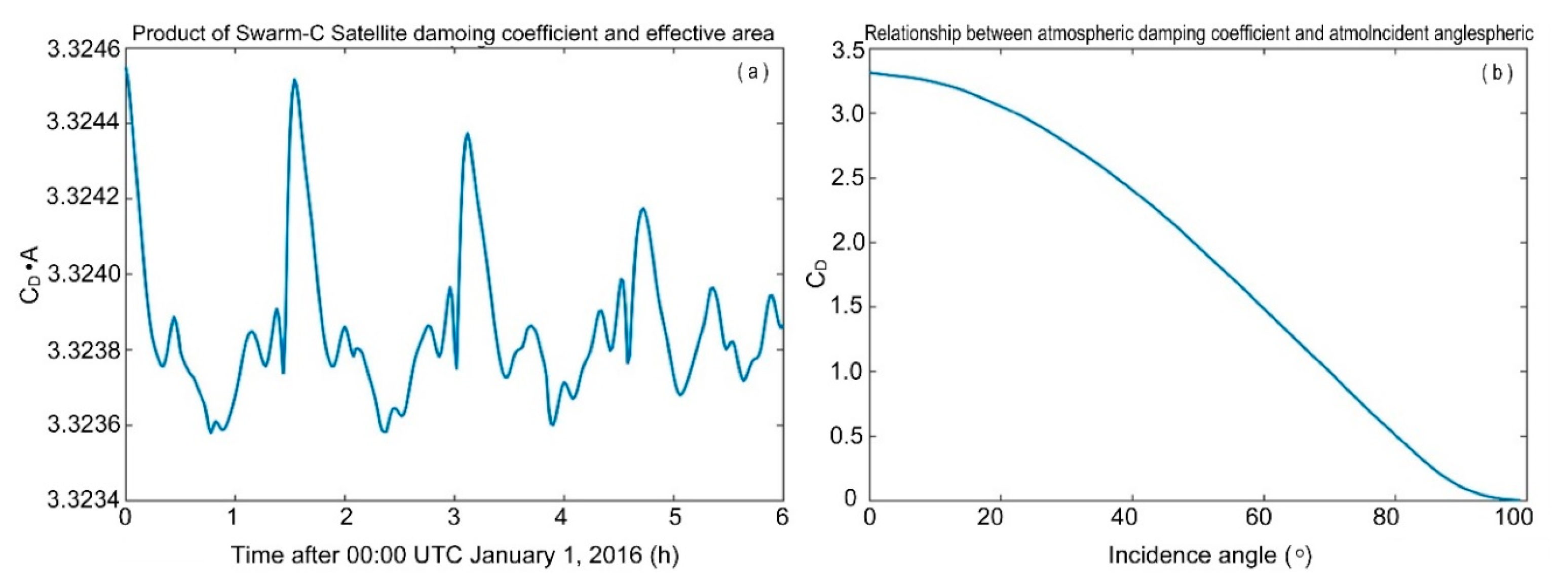
3.1. Calculation of Atmospheric Drag Coefficient of Swarm-C Satellite

Combining the atmospheric drag coefficient calculation method and the normal vector parameters of each satellite panel obtained by the abstraction of the surface shape of the Swarm-C satellite, the product of the drag coefficient and the effective area of the Swarm-C satellite was obtained. Figure 9a shows the variation of the drag coefficient’s product and the Swarm-C satellite’s effective area obtained using Equation (4).

The variation of the product of the atmospheric drag coefficient and cross-sectional area of the Swarm-C satellite with time during the day can be seen in Figure 9a. The main reason for this variation is the difference in atmospheric temperature between the daytime and night-time regions of the satellite. The atmospheric temperature has a significant effect on the drag coefficient. In addition, the different attitudes of the satellite during its orbital flight can also lead to different angles between the incident atmospheric molecules and the panel normal vectors of the satellite panels and, therefore, can impact the results [13]. Figure 9b shows the relationship between the angle of incidence of atmospheric molecules per unit area of the Swarm-C satellite and the drag coefficient.

It can be seen from Figure 9b that the large-area damping coefficient gradually decreases as the incident angle of atmospheric molecules increases from 0° to 100°. When the incident angle of atmospheric molecules is equal to 90°, the atmospheric damping coefficient is not equal to 0, and its 0 value begins to appear from around 100° on the abscissa. The reason is that the direction of the thermal motion of atmospheric molecules is random, and the direction of motion of atmospheric molecules and the direction of relative motion of the atmosphere are superimposed on each other. Therefore, when the incident angle of the atmosphere is perpendicular to the satellite panel, the velocity is not completely perpendicular to the satellite panel due to the thermal motion of atmospheric molecules.

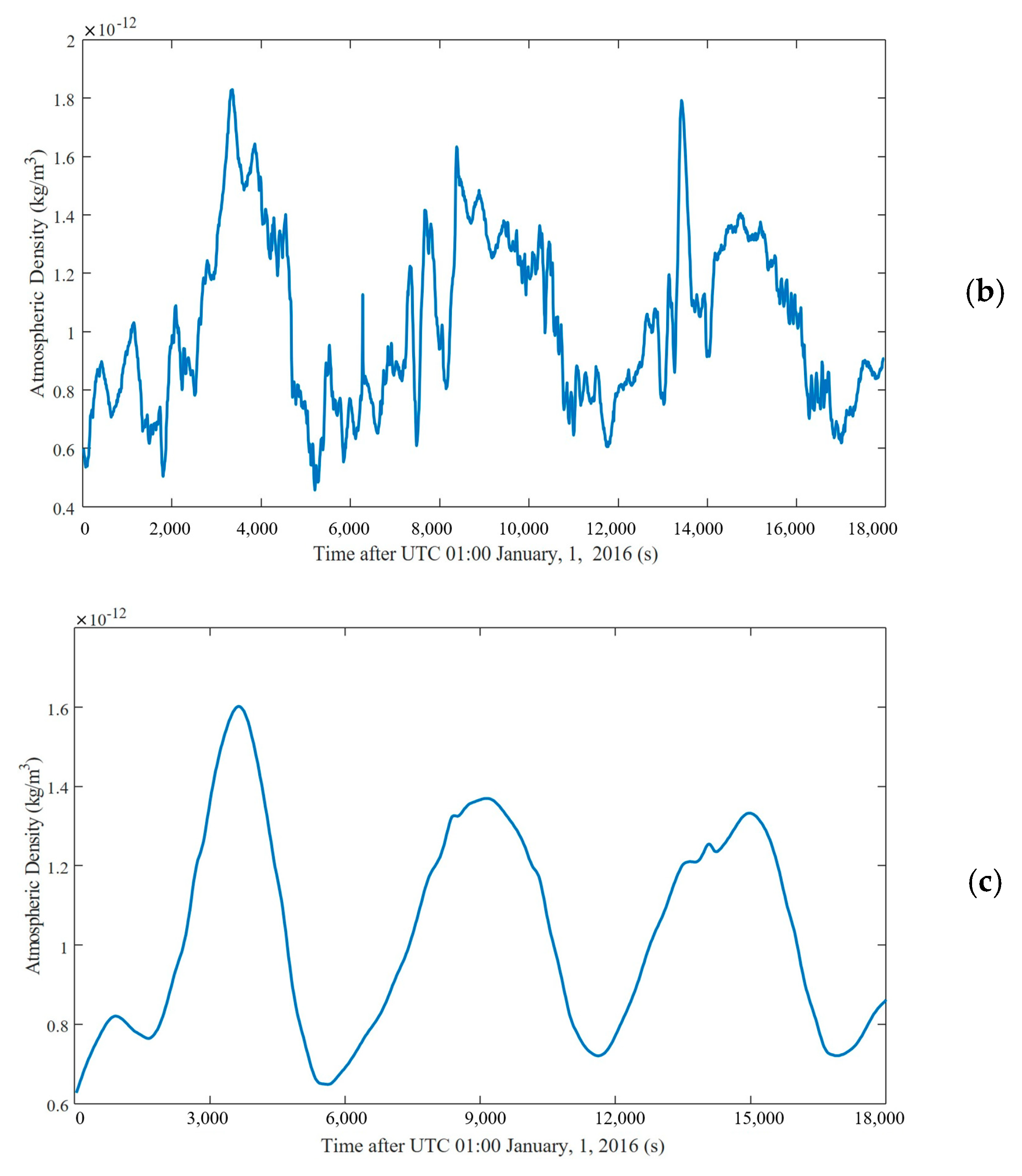
3.2. Atmospheric Density Inversion Results of Swarm-C Accelerometer

NASA researchers calculated 31 years of satellite data to obtain the average value of the bounce tract coefficient, which is a very accurate value. However, this method requires a very accurate atmospheric model. The current atmospheric model cannot guarantee accuracy in extreme environments, so obtaining the accurate value of the bounce tract coefficient in extreme environments is impossible. Therefore, in this paper, the Sentman model was used to calculate the real-time atmospheric drag coefficient instead of the average drag coefficient value, giving the later calculated atmospheric density a better real-time and dynamic performance. Since the accelerometer density on Swarm-C has been published by Siemes et al. [24] and can be retrieved, we selected the data on 1 January 2016, as a comparison. Since the accelerometer retrieval density obtained from http://thermosphere.tudelft.nl/ started at 01:00 on the 1st of January 2016, we used the data from the same period for comparison. At the same time, we also obtained the provided POD (Precise Orbit Determination) inversion density data, which were also presented in the figure. Figure 10a–c shows the thermospheric atmospheric density time series calculated by the accelerometer inversion method in this paper and the density time series published by Siemes et al.

From the time series plot presented in Figure 10, it can be seen that the atmospheric density around the orbit of the Swarm-C satellite on that date, 1 January 2016, has a magnitude of ${10}^{-12}$ kg/m³ and shows a cyclic trend with a fluctuation period of about 1.5 h, which is related to the flight trajectory of the Swarm-C satellite. Figure 10a,b illustrates that we have eliminated part of the high-frequency information in the accelerometer data correction stage; thus, the results of our inversion using the accelerometer are smoother. However, it can be seen from the results that the original characteristics of the data are preserved while correcting. We believe the correction process used is factual and does not discard the value-added properties of the high-frequency information produced by the accelerometer. It can be seen from Figure 10a and c that the density curves presented by the two are consistent in trend. Although there are numerical differences, our method retains the characteristics of the accelerometer, and the calculated density changes are more detailed.

In order to have a clearer understanding of the spatial distribution of atmospheric density at a fixed latitude, this article used the GPS precise orbit data of the Swarm-C satellite. After obtaining the time series of the thermospheric atmospheric density, the position coordinates of the Swarm-C satellite in the GPS precise orbit data were found according to the time of each item of the atmospheric density time series. Then, the time as the abscissa axis and the latitude of the satellite coordinate position as the ordinate axis was taken. Figure 11a shows the relationship diagram of the thermospheric atmospheric density changing with time at different latitudes. Since the atmospheric density time series cannot cover all times at all latitudes, it was necessary to perform interpolation on Figure 11a. We used the ordinary Kriging interpolation algorithm. Furthermore, the interpolated results are shown in Figure 11b.

Due to the limited coverage of the satellite orbit, the atmospheric density time series cannot be included at all times and at all latitudes, so the interpolation operation of the results in Figure 11a is required next.

Figure 11b shows the latitudinal time distribution of atmospheric density obtained after interpolation on Figure 10b. It can be seen that the peak of atmospheric density on that day appeared at time 2, near 50 degrees south latitude, with a peak value of about $1.6*{10}^{-12} \mathrm{kg}/{\mathrm{m}}^3$, while the minimum value appears near the northern polar region at 23:00, with a size of about $0.4*{10}^{-12} \mathrm{kg}/{\mathrm{m}}^3$. This is because the geomagnetic activity was relatively calm on this day, and no magnetic storm event occurred. For this day, the northern hemisphere was winter, and the southern hemisphere was summer.

From Figure 11b, it can be seen that the latitudinal variation of the daily average thermospheric mass density is significantly greater in the southern than in the northern hemisphere. In addition, there is a clear asymmetry in the density distribution at the North and South Poles.

4. Discussion and Conclusions

Compared with the method proposed by Siemes et al. [24], the acceleration correction method used in this research is different. Siemes et al. regarded the influence of the temperature factor as approximately linear, and this method has been proven feasible. We treat the temperature factor as linear on its basis and use the non-conservative force acceleration data derived from GPS as the calibration standard. The generalized least squares method finds calibration parameters, including deviation coefficients, scale coefficients, linear temperature factors, and trend term coefficients. After the optimal value of the calibration parameter is obtained, the corrected acceleration can be calculated. The acceleration value obtained is smoother, and the necessity of temperature correction is proved by separately showing the influence of temperature on the acceleration of Swarm-C. In the Swarm-C satellite atmospheric drag coefficient calculation experiment, the main reason for the variation of the atmospheric drag coefficient and cross-sectional area of the Swarm-C satellite products is the different atmospheric temperatures around the day and night regions. Therefore, the atmospheric temperature has a significant effect on the drag coefficient. In addition, different attitudes of the satellite during its orbital flight will result in different angles between the atmospheric molecules incident on the satellite panels and the normal vector, affecting the results. As a result of our measured atmospheric density, the peak of the curve is between $0.6*{10}^{-12}$ and $1.6*{10}^{-12}$. There is a certain difference from the inversion result using only the accelerometer because part of the peak signal is corrected, which reduces the overall digital range.

The large-area drag coefficient decreases gradually as the angle of incidence of atmospheric molecules increases. The reason is that the direction of the thermal motion of atmospheric molecules is random, and the direction of motion of atmospheric molecules and the direction of relative motion of the atmosphere are superimposed on each other. When the incident angle of the atmosphere is perpendicular to the satellite panel, due to the thermal motion of atmospheric molecules, the speed is not completely perpendicular to the satellite panel. Atmospheres with different altitudes have different compositions and temperatures, leading to different atmospheric drag coefficients. In the Swarm-C accelerometer atmospheric density inversion experiment, the latitude change of the daily average thermal mass density in the southern winter is greater than that in the northern winter. The distribution of atmospheric density in Antarctica and the Arctic has obvious asymmetry. The different positions of the magnetic poles in the northern and southern hemispheres relative to the geographic poles may cause this. Therefore, auroral heating in the southern hemisphere is more likely to produce longitudinal changes in the daily average mass density than in the northern hemisphere. Another possibility is that the asymmetry seems to be caused by solar radiation during the winter solstice.

In addition, Joule heating is proportional to ionospheric electron density and conductivity in the southern hemisphere auroral zone. As a result, the atmospheric density is higher in the southern hemisphere compared to its value in the northern hemisphere during the entire time interval considered. This phenomenon’s exact cause is unknown and needs further study.

Based on this research, we may continue to carry out research from the following aspects in the future.

(1)

Since it is impossible to know all the hardware conditions and fault causes of the Swarm-C satellite accelerometer, the accelerometer calibration method used in this paper cannot correct the errors caused by all hardware problems of the accelerometer and cannot accurately judge. Therefore, the correction scheme for the accelerometer still needs to be improved, and we also expect a higher precision correction algorithm to be developed and published by the ESA. ESA regularly publishes corrected accelerometer data from the Swarm satellites. However, the data update frequency is not high, and the time delay is relatively large. Therefore, we expect the ESA to provide higher precision corrections. This method can release the corrected accelerometer data results timelier and provide convenience for scientific researchers.

(2)

The shadow model used in this paper to calculate satellite radiation pressure only considers the projection of the Earth to the satellite. However, the Moon or other large artificial space objects can cause satellites to be projected during the operation of the satellite. When approaching the Moon and other nearby objects, the drag coefficient in that region increases as the density of surrounding particles increases due to gravitational pull. The radiation pressure of the satellite during the flight changes, so the modeling accuracy still needs to be improved. For other space objects, whether they are celestial bodies or artificial flying objects, the projection of satellites can essentially use the solar radiation model and shadow area judgment model mentioned in this paper to simulate radiation pressure. In the follow-up research, we will collect more motion trajectories of occluded objects before modeling. Suppose the trajectories of enough other space objects can be known. In that case, the accuracy of the illumination radiation pressure model used in this study will be significantly improved.

(3)

Only accelerometer data from the Swarm satellites are used in this study. The Swarm satellite’s strength lies in its ability to detect the Earth’s magnetic field changes. Therefore, the follow-up research can consider using the magnetic field data of the Swarm satellite combined with the accelerometer data for research. For example, based on magnetic field data to explore the Earth’s magnetic length anomaly and magnetic pole reversal. The influence of geomagnetic anomalies on atmospheric density is further explored based on accelerometer data and magnetic field data.

References

1. Montenbruck, O.; Gill, E.; Lutze, F. Satellite orbits: Models, methods, and applications. Appl. Mech. Rev. 2002, 55, B27–B28. [Google Scholar] [CrossRef]
2. Bowman, B. True satellite ballistic coefficient determination for HASDM. In Proceedings of the AIAA/AAS Astrodynamics Specialist Conference and Exhibit, Keystone, CO, USA, 21–24 August 2006; p. 4887. [Google Scholar]
3. Bowman, B.; Tobiska, W.K.; Marcos, F.; Huang, C.; Lin, C.; Burke, W. A new empirical thermospheric density model JB2008 using new solar and geomagnetic indices. In Proceedings of the AIAA/AAS Astrodynamics Specialist Conference and Exhibit, Keystone, CO, USA, 21–24 August 2006; p. 6438. [Google Scholar]
4. Bowman, B.R.; Tobiska, W.K.; Marcos, F.A.; Valladares, C. The JB2006 empirical thermospheric density model. J. Atmos. Solar-Terrestrial Phys. 2008, 70, 774–793. [Google Scholar] [CrossRef]
5. Moe, K.; Moe, M.M. Gas-surface interactions and satellite drag coefficients. Planet. Space Sci. 2005, 53, 793–801. [Google Scholar] [CrossRef]
6. Moe, K.; Moe, M.M. Gas-Surface Interactions in Low-Earth Orbit. In Proceedings of the AIP Conference Proceedings, Geneva, Switzerland, 15–20 September 2017; pp. 1313–1318. [Google Scholar]
7. Nwankwo, V.U.; Chakrabarti, S.K.; Weigel, R.S. Effects of plasma drag on low Earth orbiting satellites due to solar forcing induced perturbations and heating. Adv. Space Res. 2015, 56, 47–56. [Google Scholar] [CrossRef]
8. Weng, L.; Lei, J.; Doornbos, E.; Fang, H.; Dou, X. Seasonal variations of thermospheric mass density at dawn/dusk from GOCE observations. Ann. Geophys. 2018, 36, 489–496. [Google Scholar] [CrossRef] [Green Version]
9. Wang, S.; Weng, L.; Fang, H.; Xie, Y.; Yang, S. Intra-annual variations of the thermospheric density at 400 km altitude from 1996 to 2006. Adv. Space Res. 2014, 54, 327–332. [Google Scholar] [CrossRef]
10. Newton, G.P.; Horowitz, R.; Priester, W. Atmospheric density and temperature variations from the explorer XVII satellite and a further comparison with satellite drag. Planet. Space Sci. 1965, 13, 599–616. [Google Scholar] [CrossRef]
11. Calabia, A.; Jin, S. Thermospheric density estimation and responses to the March 2013 geomagnetic storm from GRACE GPS-determined precise orbits. J. Atmos. Solar-Terrestrial Phys. 2017, 154, 167–179. [Google Scholar] [CrossRef]
12. Drob, D.; Emmert, J.; Crowley, G.; Picone, J.; Shepherd, G.; Skinner, W.; Hays, P.; Niciejewski, R.; Larsen, M.; She, C. An empirical model of the Earth’s horizontal wind fields: HWM07. J. Geophys. Res. Space Phys. 2008, 113, 18. [Google Scholar] [CrossRef] [Green Version]
13. Picone, J.; Hedin, A.; Drob, D.P.; Aikin, A. NRLMSISE-00 empirical model of the atmosphere: Statistical comparisons and scientific issues. J. Geophys. Res. Space Phys. 2002, 107, SIA 15-11–SIA 15-16. [Google Scholar] [CrossRef]
14. Emmert, J. Altitude and solar activity dependence of 1967–2005 thermospheric density trends derived from orbital drag. J. Geophys. Res. Space Phys. 2015, 120, 2940–2950. [Google Scholar] [CrossRef]
15. Calabia, A.; Jin, S. New modes and mechanisms of thermospheric mass density variations from GRACE accelerometers. J. Geophys. Res. Space Phys. 2016, 121, 11191–111212. [Google Scholar] [CrossRef]
16. Menvielle, M.; Lathuillere, C.; Bruinsma, S.; Viereck, R. A new method for studying the thermospheric density variability derived from CHAMP/STAR accelerometer data for magnetically active conditions. Ann. Geophys. 2007, 25, 1949–1958. [Google Scholar] [CrossRef]
17. Zurek, R.; Tolson, R.; Bougher, S.; Lugo, R.; Baird, D.; Bell, J.; Jakosky, B. Mars thermosphere as seen in MAVEN accelerometer data. J. Geophys. Res. Space Phys. 2017, 122, 3798–3814. [Google Scholar] [CrossRef]
18. Bruinsma, S.; Tamagnan, D.; Biancale, R. Atmospheric densities derived from CHAMP/STAR accelerometer observations. Planet. Space Sci. 2004, 52, 297–312. [Google Scholar] [CrossRef]
19. Sutton, E.K. Effects of Solar Disturbances on the Thermosphere Densities and Winds from CHAMP and GRACE Satellite Accelerometer Data; University of Colorado at Boulder: Boulder, CO, USA, 2008. [Google Scholar]
20. Doornbos, E.; Van Den Ijssel, J.; Luhr, H.; Forster, M.; Koppenwallner, G. Neutral density and crosswind determination from arbitrarily oriented multiaxis accelerometers on satellites. J. Spacecr. Rocket. 2010, 47, 580–589. [Google Scholar] [CrossRef] [Green Version]
21. Emmert, J.; McDonald, S.; Drob, D.; Meier, R.; Lean, J.; Picone, J. Attribution of interminima changes in the global thermosphere and ionosphere. J. Geophys. Res. Space Phys. 2014, 119, 6657–6688. [Google Scholar] [CrossRef]
22. Mehta, P.M.; Walker, A.C.; Sutton, E.K.; Godinez, H.C. New density estimates derived using accelerometers on board the CHAMP and GRACE satellites. Space Weather 2017, 15, 558–576. [Google Scholar] [CrossRef]
23. Visser, P.; Doornbos, E.; van den IJssel, J.; da Encarnação, J.T. Thermospheric density and wind retrieval from Swarm observations. Earth Planets Space 2013, 65, 1319–1331. [Google Scholar] [CrossRef] [Green Version]
24. Siemes, C.; de Teixeira da Encarnação, J.; Doornbos, E.; Van Den Ijssel, J.; Kraus, J.; Pereštý, R.; Grunwaldt, L.; Apelbaum, G.; Flury, J.; Holmdahl Olsen, P.E. Swarm accelerometer data processing from raw accelerations to thermospheric neutral densities. Earth Planets Space 2016, 68, 92. [Google Scholar] [CrossRef] [Green Version]
25. Bezděk, A. Calibration of accelerometers aboard GRACE satellites by comparison with POD-based nongravitational accelerations. J. Geodyn. 2010, 50, 410–423. [Google Scholar] [CrossRef] [Green Version]
26. Bezděk, A.; Sebera, J.; Klokočník, J. Calibration of Swarm accelerometer data by GPS positioning and linear temperature correction. Adv. Space Res. 2018, 62, 317–325. [Google Scholar] [CrossRef]
27. Saad, N.A.; Khalil, K.I.; Amin, M.Y. Analytical solution for the combined solar radiation pressure and luni-solar effects on the orbits of high altitude satellites. Open Astron. J. 2010, 3, 113–122. [Google Scholar] [CrossRef]
28. Srivastava, V.K.; Ashutosh, A.; Roopa, M.; Ramakrishna, B.; Pitchaimani, M.; Chandrasekhar, B. Spherical and oblate Earth conical shadow models for LEO satellites: Applications and comparisons with real time data and STK to IRS satellites. Aerosp. Sci. Technol. 2014, 33, 135–144. [Google Scholar] [CrossRef]
29. Moe, M.M.; Wallace, S.D.; Moe, K. Errata: Refinements in Determining Satellite Drag Coefficients: Method for Resolving Density Discrepancies. J. Guid. Control. Dyn. 1993, 16, 0991b. [Google Scholar] [CrossRef]
30. Sentman, L.H. Free Molecule Flow Theory and Its Application to the Determination of Aerodynamic Forces; Lockheed Missiles and Space Co Inc Sunnyvale Ca: Sunnyvale, CA, USA, 1961. [Google Scholar]
31. Van den IJssel, J.; Encarnação, J.; Doornbos, E.; Visser, P. Precise science orbits for the Swarm satellite constellation. Adv. Space Res. 2015, 56, 1042–1055. [Google Scholar] [CrossRef]
32. Ren, T.; Miao, J.; Liu, S. Atmospheric density determination using high-accuracy satellite GPS data. Sci. China Technol. Sci. 2018, 61, 204–211. [Google Scholar] [CrossRef]
33. Wöske, F.; Kato, T.; Rievers, B.; List, M. GRACE accelerometer calibration by high precision non-gravitational force modeling. Adv. Space Res. 2019, 63, 1318–1335. [Google Scholar] [CrossRef]
34. Calabia, A.; Jin, S.; Tenzer, R. A new GPS-based calibration of GRACE accelerometers using the arc-to-chord threshold uncovered sinusoidal disturbing signal. Aerosp. Sci. Technol. 2015, 45, 265–271. [Google Scholar] [CrossRef]
35. Koch, I.; Shabanloui, A.; Flury, J. Calibration of GRACE Accelerometers Using Two Types of Reference Accelerations. In Proceedings of the International Symposium on Advancing Geodesy in a Changing World, Kobe, Japan, 30 July–4 August 2017; pp. 97–104. [Google Scholar]
36. Klinger, B.; Mayer-Gürr, T. The role of accelerometer data calibration within GRACE gravity field recovery: Results from ITSG-Grace2016. Adv. Space Res. 2016, 58, 1597–1609. [Google Scholar] [CrossRef] [Green Version]
Figure 1. The main workflow of this study.
Applsci 13 03610 g001
Figure 2. Comparison before and after preprocessing and correcting Swarm-C satellite data. (a) Peak signal processing; (b) EDAC fault signal processing.
Applsci 13 03610 g002
Figure 3. Comparison of Swarm-C satellite accelerometer data before and after correction.
Applsci 13 03610 g003
Figure 4. Comparison between accelerometer data correction results and ESA (a) during magnetic storm day (Kp = 8, magnetic storm level: G4); (b) during nonmagnetic storm day.
Applsci 13 03610 g004
Figure 5. Simplified satellite parameters. (a) Simplified shape model of Swarm-C satellite; (b) schematic diagram of the side panel and bottom panel of Swarm-C satellite.
Applsci 13 03610 g005
Figure 6. Schematic diagram of conical shadow model.
Applsci 13 03610 g006
Figure 7. Light radiation acceleration (LRA) when Swarm-C after full-shadowed. (a) LRA along the orbit; (b) LRA in orthogonal directions; (c) LRA in the radial direction.
Applsci 13 03610 g007
Figure 8. Comparison of conical shading model modeling and column shading modeling.
Applsci 13 03610 g008
Figure 9. The Swarm-C satellite coefficient relationships. (a) Swarm-C satellite drag coefficient and effective area product; (b) atmospheric drag coefficient versus angle of incidence of gas molecules.
Applsci 13 03610 g009
Figure 10. Atmospheric density time series obtained from Swarm-C satellite accelerometer data. (a) Our method; (b) accelerometer inversion results; (c) POD inversion results.
Applsci 13 03610 g010aApplsci 13 03610 g010b
Figure 11. Time–latitude distribution of atmospheric density on 1 January 2016. (a) Before interpolation; (b) after interpolation.
Applsci 13 03610 g011