Article

Optimal Power Flow Solutions for Power System Considering Electric Market and Renewable Energy

by
Thang Trung Nguyen
1,
Hung Duc Nguyen
2,3,* and
Minh Quan Duong
4,*
1
Power System Optimization Research Group, Faculty of Electrical and Electronics Engineering, Ton Duc Thang University, Ho Chi Minh City 700000, Vietnam
2
Department of Power Delivery, Ho Chi Minh City University of Technology (HCMUT), 268 Ly Thuong Kiet Street, District 10, Ho Chi Minh City 700000, Vietnam
3
Vietnam National University Ho Chi Minh City, Linh Trung Ward, Thu Duc City, Ho Chi Minh City 700000, Vietnam
4
The University of Danang-University of Science and Technology, Danang 550000, Vietnam
*
Authors to whom correspondence should be addressed.
Appl. Sci. 2023, 13(5), 3330; https://doi.org/10.3390/app13053330
Submission received: 3 February 2023 / Revised: 27 February 2023 / Accepted: 3 March 2023 / Published: 6 March 2023
(This article belongs to the Topic Exergy Analysis and Its Applications – 2nd Volume)

Abstract

:
The paper applies jellyfish search algorithm (JSA) for reaching the maximum profit of IEEE 30-node and IEEE 118-node transmission power networks considering electrical market and wind turbines (WTs). JSA is compared with the particle swarm optimization (PSO), genetic algorithm (GA), moth swarm algorithm (MSA), salp swarm algorithm (SSA), and water cycle algorithm (WCA) for three study cases. The same and different electric prices for all nodes are, respectively, considered in Case 1 and Case 2, whereas Case 3 considers different prices and the placement of one WT. As a result, JSA can reach higher profit than MSA, SSA, WCA, PSO, and GA by 1.2%, 2.44%, 1.7%, 1.3%, and 1.02% for Cases 1, 2, and 3. Then, JSA is applied for optimizing the placement of from two to four WTs for the first system, and from zero to five wind farms (WF) for the second systems. Comparison of profits from the study cases indicates that the network can reach higher profit if more WTs and WFs are optimally placed. The placement of four WTs can support the two systems to reach higher profit by $130.3 and $34770.4, respectively. The greater profits are equivalent to 2.6% and 97.2% the profit of the base system. On the other hand, the obtained results also reveal the important order of location for installing wind power generators. The important order of nodes is, respectively, Nodes 5, 2, 1, and 10 for the first system, as well as Nodes 29, 31, 71, 45, and 47 for the second system. Thus, it is recommended that renewable energies are very useful in improving profit for transmission power systems, and the solutions of installing renewable energy-based generators should be determined by high performance algorithms, such as JSA.

1. Introduction

Optimal power flow (OPF) is a very important for power systems to reach stable and economic operation statuses. Control parameters of electric components in the power system must be set appropriately to assure that other components’ parameters can be within an allowable working range [1]. The purpose can be reached by running the OPF program for power systems, so OPF is one of the leading problems in power system operation fields. Basically, the power system is comprised of three major parts, high capacity power plants, transmission power networks and distribution power networks in which the OPF problem has been studied so far for increasing the effectiveness of high capacity power plants and the transmission of power grids [2]. In conventional OPF problems, core power sources are mainly thermal power plants, which are mainly dependent on fossil fuels such as coal, gas, and oil. In recent years, renewable energy-based power plants, such as solar, photovoltaic, and wind power plants, have been concerned as a part of power source in power systems where major thermal power plants had been working stably on their sites. Thus, the new OPF problem with the presence of renewable energy-based power plants focuses on the determination of location and capacity for the renewable energy-based power plants. To solve the conventional OPF problem, optimization tools, such as deterministic algorithms and metaheuristic algorithms, find the control parameters of the power system and voltage of all generators, active power of generators, excluding slack, reactive power output of capacitors, and tap setting of transformers. Then, the Matpower program is run to reach other remaining parameters, such as active power of slack generator, reactive power of all generators, apparent power of lines, and voltage of loads [3]. As all parameters are within a predetermined operation range, the OPF solutions obtained are valid and they can be acknowledged for reaching stable operation status [4]. However, they may not be effective solutions. Derived from an unexpected issue, many methods have been proposed and evaluated so far [5]. For dealing with the new OPF problem, the duty of optimization tools is more difficult, since they must determine three more factors of renewable energy-based power plants, such as the number of added power plants, the location, and the capacity of each added power plant.
For solving such conventional OPF problems, classical methods and numerical methods, such as gradient search algorithm [1], quadratic programming [5], Newton method [6,7], linear programming [8,9], nonlinear programming [10], and interior point [11], were applied in the past, as metaheuristic algorithms were not highly developed and widely applied. These methods had the same ideal as using an optimization function based on Lagrange multipliers, and they had the objective of taking partial derivative to reach control parameters and dependent parameters of the problem. They are deterministic methods, so they reach the same solutions for different trial runs. Meta-heuristic algorithms differ from the conventional optimization approaches in principle, so their performance for OPF problems is also different from that of the above conventional ones [12]. The metaheuristic optimization approaches are able to implement the non-deterministic optimal search based on randomization and solution update mechanisms without using derivative implementation. The fitness function is a very important factor of these metaheuristic algorithms in dealing with all constraints and reaching high quality of control variables. Normally, the fitness function is comprised of two terms, objective function that needs to be optimized and penalty terms for satisfying all constraints. If the two terms are selected unsuitably, metaheuristic algorithms will not reach valid solutions meeting all constraints and high-quality objective functions. Researchers can find new fitness functions for reducing difficulty for applied algorithms or reaching more effective solutions more easily. Therefore, the applications of the metaheuristics are more and wider than other deterministic conventional algorithms. Almost metaheuristic algorithms can solve the OPF successfully, in which modified or hybrid algorithms can reach better results, such as the lightning attachment procedure algorithm [13], pattern search technique based particle swarm optimization [14], hybrid evolutionary algorithm [15], modified crossover based differential evolution [16], manta ray foraging optimizer [17], hybrid whale algorithm, moth–flame algorithm [18], improved Archimedes optimization algorithm [19], moth–flame optimization algorithm [20], and adaptive Gaussian teaching–learning algorithm [21]. In general, these studies focused on improving original metaheuristic algorithms for better performance or improving constraint handling methods for satisfying limitation of dependent variables, rather than improving power flow tools, such as Newton-Raphson and Gauss-Seidel. Different objective functions were optimized for comparison and evaluation of performance.
Recently, researchers have concerned renewable power plants in transmission power grids, and the OPF problem has become more complicated by the presence of the plants. Major factors of the renewable plants are the number of added plants, installed location, and rated power for each added plant. So, to solve the OPF problem with the installation of renewable energies, there are major factors that must be accomplished before finding important parameters of basic electric components, such as thermal units, capacitors, transformers, loads, and transmission branches, as mentioned above. Basically, researchers are supposed to install small WFs and PVSs from some to tens of megawatts. The studies focused on two topics, including (1) the placement of WFs [22,23,24,25,26,27] and (2) the placement of both PVSs and WFs [28,29,30,31,32,33,34,35,36,37,38]. These studies have used different metaheuristic algorithms and solved at least one standard IEEE transmission network with 30 nodes and at most three standard IEEE systems with 30, 57, and 118 nodes. Information of the studies consisting of algorithms, applied systems, objective function, number of renewable units, location, and power of each unit is given in Table 1. Almost all studies used only WFs or both WFs and PVSs rather than only PVSs. Popular nodes for the placement of renewable energy are 3 and 30, or 10 and 24 for the IEEE 30-node system. For the IEEE 57 and 118-nodes systems, the location is not the same for studies. One study [24] used the loss sensitivity factor-based method to determine node 30 and node 3, which are the most and the least important for installing distributed generators based on solar radiation or wind. Then, the Jaya algorithm was applied to optimize rated power of WFs and parameters of other electric components. The results indicated that node 30 was more suitable than node 3 for placing WFs. Some of the studies used the determined locations to optimize size of WFs [25,26], meanwhile others optimized both location and size [27,28,29], and others optimized three factors, including the number of units, location, and power of each unit [33,34,35,36,37,38]. Almost all methods focused on fuel cost minimization, loss minimization, and voltage improvement.
Another topic of the OPF problem is to consider the stochastic participation of renewable energy sources in transmission power networks. The flow direction algorithm was applied in [39] to reduce the total operating cost for all power plants, such as thermal, small hydro, wind, and solar photovoltaic power plants. The study has suggested that the total cost could be minimum if the energy efficiency was maximized by increasing stochastic participation of the renewable power plants, wind farms, and photovoltaic fields. Three standard IEEE systems with 30, 57, and 118 nodes were employed for simulation. The study [40] has applied the mayfly algorithm to minimize several single objectives, such as total cost of wind, solar and thermal power plants, voltage deviation, power loss, and emission for a 30-node transmission power network. In one study [41], the gorilla troop algorithm was run for two systems with 30 and 118 nodes for reaching the smallest cost of thermal units only. In general, the three algorithms have tried to reduce the total generation cost, but they had different ideas of cost. The two studies [39,40] have considered the cost of renewable energies, but another study [41] has ignored the cost. However, the three studies have pointed out that, as the uncertainty of renewable energies was high, the cost of generation could be higher due to the use of more power from thermal power plants.
In this study, we optimized power flow for the IEEE 30-node and IEEE-118 node power networks considering nodal prices and placement of wind energy-based generators. The different nodal prices are considered to optimize the location and rated power of wind farms installed in the system. The study [42] has built a set of generators and run nodal price program to calculate electricity price for the first system. To simulate the two systems, JSA [43], MSA [44], SSA [45], WCA [46], PSO [47], and GA [48] are implemented for find the most solutions. In summary, the novelties of the paper can be expressed as follows:
  • Applying different nodal prices for nodes in transmission power networks and considering wind energy. The study is more complicated than previous studies [22,23,24,25,26,27,28,29,30,31,32,33,34,35,36,37,38] by considering the node prices, and it is also more complicated than the previous study [38] by considering wind energy.
  • Consider different number of wind turbines and wind farms. In the first system with 30 nodes, four study cases of WTs placement with one, two, three and four WTs in range between 0 MW and 10 MW are implemented. In the second system with 118 nodes, five study case of WFs placement, from one to five WFs in range from 0 to 100 MW are simulated. Two factors of each wind turbine as well as each wind farm must be determined, including the placed location and rated power. The different study cases aim to determine the most suitable nodes to place wind energy as joining electric market. The target has not been concerned in all previous studies.
  • Applying recent and effective metaheuristic algorithms, including JSA [43], MSA [44], SSA [45], WCA [46], PSO [47], and GA [48]. There are conventional and novel algorithms in the six applied ones.
The contributions of the paper are as follows:
  • Reach optimal solutions of placing wind turbines in the IEEE 30-node and the IEEE 118-node transmission power networks in electric market.
  • Find the maximum profit of electricity sale for the case without and with wind energy. The obtained maximum profits indicate the most suitable nodes for installing wind turbines and the most effective number of WTs and WFs for reaching the highest profit. On the other hand, the priority order of nodes for placing wind energy-based generators can be used to plan stability improvement for the transmission power networks.
  • Find one suitable metaheuristic algorithm for all study cases with electric market and wind energy. The six algorithms have applied for different optimization problems so far; however, the most powerful one should be recommended for other similar studies.
Other parts of the paper are as follows: Section 2 shows objective function and all requirement conditions. Section 3 presents the structure of JSA and the whole solution process of JSA for the problem. Section 4 presents the results obtained by four applied algorithms for study cases. Section 5 summarizes the obtained results, contributions, shortcomings, and proposes future work to tackle the shortcomings.

2. Formulation of the Studied Problem

The study focuses on the profit maximization for transmission power networks considering different prices of nodes in the networks and the placement of wind turbines. Thermal power plants must consume fossil fuels to produce and supply electricity to loads. Conventional studies of the OPF problem have ignored the prices at load nodes, and this neglection has not considered the effectiveness of different thermal power plants in power systems. For recent OPF problems considering renewable energies, the neglection has been seen again. So, the study has focused on the maximization of profit for the transmission power networks considering nodal prices and renewable energy, which is supposed to be wind turbines. The objective and constraints are presented as follows:

2.1. Objective Functions

Total cost of thermal power plants: basically, a power system consists of a number of generators using fossil fuels for generation process. The fossil fuel cost is regarded as an investment cost meanwhile total revenue from electricity sale for loads is the sum of cost and profit. The profit is very important for operation of transmission power networks, and it must be maximized. The maximization of the profit is the objective of the study, and it is expressed as follows:
Maximize   S y s P r o f i t = T o R e E l e c C o s t F u e l  
C o s t F u e l and T o R e E l e c are basically obtained by:
C o s t F u e l = k = 1 N T U s c e 1 k + c e 2 k P T k + c e 3 k ( P T k ) 2
T o R e E l e c = l = 1 N L o a d s E P r l . P L o a d l

2.2. Constraints

Power balance: The balance of power between the source (i.e., power generated by thermal units, wind power plants, and capacitors) and consumption (i.e., demands of all loads and losses on all transmission lines) is a common restriction. The constraint is for active power and reactive power as follows:
k = 1 N T U s P T k + m = 1 N W P s P W m   l = 1 N L o a d s P L o a d l b = 1 N B r s P L o s s , b = 0
k = 1 N T U s Q T k + c = 1 N C a p s Q C c + m = 1 N W P s Q W m    l = 1 N L o a d s Q L o a d l b = 1 N B r s Q L o s s , b = 0
However, the constraints (4) and (5) cannot be reached directly by power flow method, Newton-Raphson. The Matpower program [49] is used in the study to reach power flows, and the program uses the Newton-Raphson method [50]. The two general constraints are converted into the balance power constraint at each node as follows:
  P T i   +   P W i   P L o a d i = V o l i j N n o d e s V o l j [ G C i j cos ( θ i - θ j ) + B S i j sin ( θ i - θ j )   ] ;   i = 1 , ,   N n o d e s
  Q T i   + Q C i   - Q L o a d i = V o l i j N n o d e s V o l j [ G C i j cos ( θ i - θ j )   B S i j sin ( θ i - θ j )   ] ;   i = 1 , ,   N n o d e s
where QCi is the reactive power generation of the capacitors at the ith node and QCi must be constrained by:
Q C i M i n   Q C i   Q C i M a x   ; i = 1 , ,   N n o d e s  
Limitation on active and reactive power generation: As operating, thermal units and wind power plants must satisfy the limitation of active and reactive generation capacity as follows:
P T k M i n   P T k     P T k M a x      
  P W m   M i n   P W m     P W m   M a x
Q T k M i n   Q T k     Q T k M a x
Q W m   M i n   Q W m     Q W m   M a x
Limitation on voltage: All loads and generators at the ith node must be kept within an acceptable operating range, as follows:
V o l i M i n V o l i   V o l i M a x ;   i = 1 , ,   N n o d e s
V o l k M i n V o l k   V o l k M a x ;   k = 1 , ,   N T U s
where V o l i M i n and V o l i M a x , and V o l k M i n and V o l k M a x are the smallest and highest voltage values of load at the node i and of the thermal unit k. In the study, the two values are selected to be 0.95 and 1.1 pu, respectively [4].
Transformer constraints: The transformer’s tap setting must fall within the lower and upper limits indicated by the inequality below:
T p M i n   T p n     T p M a x   ;   n = 1 , ,   N T F  
Limitation of transmission lines: Transmission lines are conductors connecting each two nodes. The transmission limit of the lines is also the limit of the conductors. However, parameter of transmission lines is apparent power, while that of conductors is current. So, the current limit must be converted into apparent power limit as follows:
  S b     S b M a x   ;   b = 1 , ,   N B r s  
where   S b   and   S b M a x are the operating apparent power and the maximum capacity of the bth transmission line.

3. Jellyfish Search Algorithm for the Problem

Jellyfish algorithm (JSA) was developed by Chou, J. S. and Truong, D. N. in 2020 by taking the idea from the jellyfish’s movements in the ocean [43]. The structure of JS is not as complicated as the genetic algorithm, water cycle algorithm, etc. In fact, JSA is comprised of the same techniques as simple metaheuristic algorithms, such as initialization and selection technique, and it is only different from others about the process of searching new solutions. The structure and application of JSA for the considered problem are presented as follows:

3.1. Jellyfish Algorithm (JS)

Similar to the flower pollination algorithm [51], JSA also uses two techniques, called exploration and exploitation, to search new solutions. However, only one out of the two methods is used for each iteration based on the comparison between a decision parameter at the current iteration and a balance parameter. For simplicity, the balance parameter can be fixed at 0.5 for simplicity, whereas the decision parameter is dependent on the current iteration and maximum iteration as follows:
C P G p r e = ( 1 G p r e G m a x ) × ( d r 0 2 1 )
where C P G p r e is the decision parameter at the present iteration G p r e . Equation (17) indicates that C P G p r e has one value only at each iteration. So, the comparison of ( C P G p r e and 0.5) leads to one result only and only one method is used for each iteration.
If C P G p r e is smaller than 0.5, the whole population is updated based on the exploration technique, as shown in the following formula:
S N j n e w = S N j + d r 1 . ( S N * 3 . d r 2 . S N m i d ) ,   j = 1 ,   ,   S s i z e
For other case (i.e., 0.5 < C P G p r e ), exploitation technique is used to update the solution at the present iteration as the following equation:
S N j n e w = { S N j + Δ j ,                                              if   r d n . ( 1 C P G p r e ) d r 3 S N j + d r 0 0.1 . ( U p L L o L ) ,              else  
where Δ j is a distance between the jth old solution the jth new solution, which is obtained by one out of two ways as follows:
Δ j = { S N j S N r d ,          if   F i t r d < F i t j S N r d S N j ,            else  

3.2. The Implementation of JSA for the Problem

3.2.1. The Selection of Control Variables

JSA and other applied metaheuristic algorithms have a responsibility for producing high quality control variables for the considered OPF problem. The obtained control variables are normally evaluated by evaluating fitness function of solutions in which fitness function has two main parts, objective, and penalty. Objective function may be a function of dependent variables or control variables, or both. Meanwhile, penalty terms indicate the violation of all dependent variables. In this problem, there are seven control variables—three from wind farms and four others from other electric components. They are listed as follows:
  • Location of wind turbines: L W P m where m = 1 ,   ,   N W P s . Each wind turbine can be located at the smallest node number (node 1) and the highest node number (Node N n o d e s ). So, Node 1 and Node N n o d e s are, respectively, the minimum and maximum locations, which are represented by L W P m M i n and L W P m M a x .
2.
Rated power of wind turbines: P W m   (   m = 1 ,   ,   N W P s ) .
3.
Power factor of wind turbines: P F W P m ( m = 1 ,   ,   N W P s ).
4.
Active power generation of all thermal units excluding that in slack node: P T k ( k = 2 , ,   N T U s ). It is supposed that the first thermal unit (i.e., k = 1) is located at the slack node.
5.
Tap of transformers:   T p n   ( n = 1 , ,   N T F ).
6.
Reactive power generation of all capacitors: Q C c (c = 1, …, N C a p s ).
7.
Voltage magnitude of all thermal units: V o l k ( k = 1 , ,   N T U s ).

3.2.2. The Calculation of Dependent Variables

To reach dependent variables of the problem, location, rated active power, and power factor of each wind farm are produced by using JSA. Then, data of the system are modified by adding the three factors into the original data. Finally, the Matpower program [49] is run for reaching dependent variables. The dependent variables are listed as follows:
  • Active power generation of thermal unit at slack node: P T 1 .
2.
Reactive power generation of all thermal units: Q T k ( k = 1 , ,   N T U s ).
3.
Apparent power of all branches:   S b   ( b = 1 , ,   N B r s ).
4.
Voltage of all loads: V o l i ( i = 1 , ,   N n o d e s ).

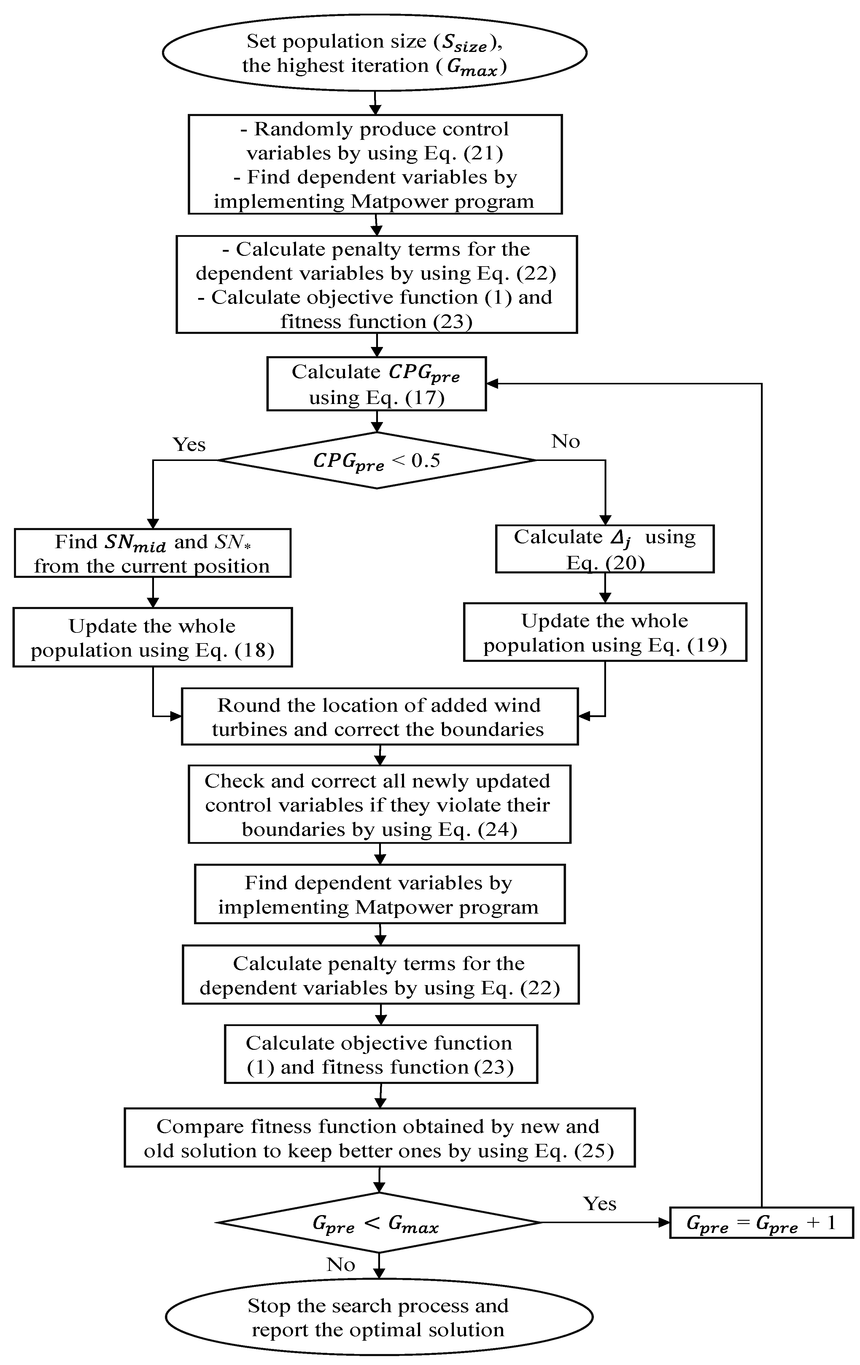
3.3. The Implementation of JSA for the Considered OPF Problem

The section presents an iterative technique to apply JSA for the considered OPF problem with the presence of renewable energy and the consideration of different nodal prices. The implementation process is expressed as the following steps:
  • Step 1: Generate initial solutions.
Each solution S N j of JSA is comprised of the set of control variables presented in Section 3.2.1. To produce a random initial population for JSA, the lower and upper boundaries of the solution S N j are formed as follows: S N j M i n and S N j M a x . The lower boundary S N j M i n is comprised of the minimum value of all control variables meanwhile the upper boundary S N j M a x is comprised of the maximum value of all control variables. In the first step, we randomly produce the population as follows:
S N j = d r 3 . ( S N j M a x S N j M i n ) + S N j M i n ;   j = 1 ,   ,   S s i z e
  • Step 2: Obtain all dependent variables and penalize their violation.
In the second step, all remaining dependent variables are obtained by using Section 3.2.2. These variables are included in a set of dependent variables, which is mathematically modeled by D S j . Each dependent variable can be either within or beyond its allowable range, which is predetermined and normally is given in data of the system. Similar to the control set, the dependent set also has the lower and upper boundaries, which are represented by D S j M i n and D S j M a x . The two boundaries are, respectively, comprised of the minimum and maximum values of all dependent variables. If the dependent variables have smaller value than the lower bound, they are penalized by calculating the deviation between the obtained value and the lower bound. For another case of violation, if the dependent variables have greater value than the upper bound, the deviation between the obtained value and the upper bound is calculated for the penalty. By using the way, penalty terms of all dependent variables are calculated as follows:
Δ D S j = { 0     if   Δ D S j [ D S j M i n ;   D S j M a x ]    ( D S j M i n D S j )           if   D S j < D S j M i n ( D S j D S j M a x )          if   D S j > D S j M a x
  • Step 3: Calculate fitness function of all solutions.
Currently, all variables of the problem are obtained and currently the objective function (1) can be calculated simply. The penalty terms above and the objective function are included in fitness function as follows:
F i t j = S y s P r o f i t , j + β . ( Δ D S j ) 2
where S y s P r o f i t , j is the objective function of the jth solution; and β is an intensification factor. β is used to make the violation of dependent variables greater and selected to be 104 in the paper by experiment.
  • Step 4: Produce and correcting new control variables by using JSA.
In this step, the search process of JSA in Section 3.1 is applied to find new solutions containing new control variables. However, all new obtained control variables can be within or beyond their predetermined boundaries. Before performing Matpower program for reaching dependent variables, the new variables must be repaired as follows:
S N j n e w = { S N j n e w     if   S N j M i n   S N j n e w   S N j M a x    S N j M i n           if   S N j M i n > S N j n e w S N j M a x           if    S N j M a x < S N j n e w
  • Step 5: Implement selection of better-quality variables and find the best solution.
Currently, there are two solutions corresponding to two sets of control variables for each individual in the population. In other words, there are two population, old and new. So, the jth old and the jth new variable set should be selected to abandon one set and keep one set. The fitness function of each new variable set is represented by F i t j n e w . Meanwhile, that of each old variable set is still F i t j . The selection is implemented by using the following model:
S N j = { S N j n e w     if    F i t j n e w   F i t j S N j         else
Finally, the best solution with the smallest fitness function is determined, and its parameters, such as objective function, control variables, and dependent variables are stored.
These computation steps are applied in Figure 1 to show the detailed implementation of JSA for the considered OPF problem.

4. Numerical Results

4.1. Applied Algorithms and Test Systems

In this section, we apply metaheuristic algorithms for finding the best solution of installing wind turbines in the standard IEEE 30-node and IEEE 118-node systems. The configuration of the two systems is shown in Figure 2 and Figure 3. Data of the transmission networks and cost coefficients of thermal units are taken from the study [4]. The nodal prices of the first system are taken from [42], while the nodal prices of the second system are first developed in the study. The prices are shown in Table A1 and Table A2 in Appendix A. The simulation is executed on a personal computer with s 2.4 Ghz processor, 8 GB of RAM, and using the Matlab program. In addition, the Matpower program is applied to find dependent variables.
For the first system, there are five study cases, but only the first three cases are implemented by six algorithms, JSA, MSA, SSA, WCA, PSO, and GA. Each method is run for 50 trials for each case, and then the best algorithm is run for two remaining cases, Case 4 and Case 5. The five cases are as follows:
Case 1: Consider the same price of $25 for all nodes in the system and neglect wind turbine placement.
Case 2: Consider the different electric price for different nodes and neglect wind turbine placement.
Case 3: Consider different electric prices for different nodes and optimal placement of one wind turbine.
Case 4: Consider different electric prices for different nodes and use the optimal placement of one turbine of Case 3.
Case 5: Consider different electric prices for different nodes and optimal placement of two, three, and four wind turbines.
For the second system, only JSA is run for six study cases with different nodal prices and different number of WFs. The whole simulation cases of the two systems are summarized in Table 2.

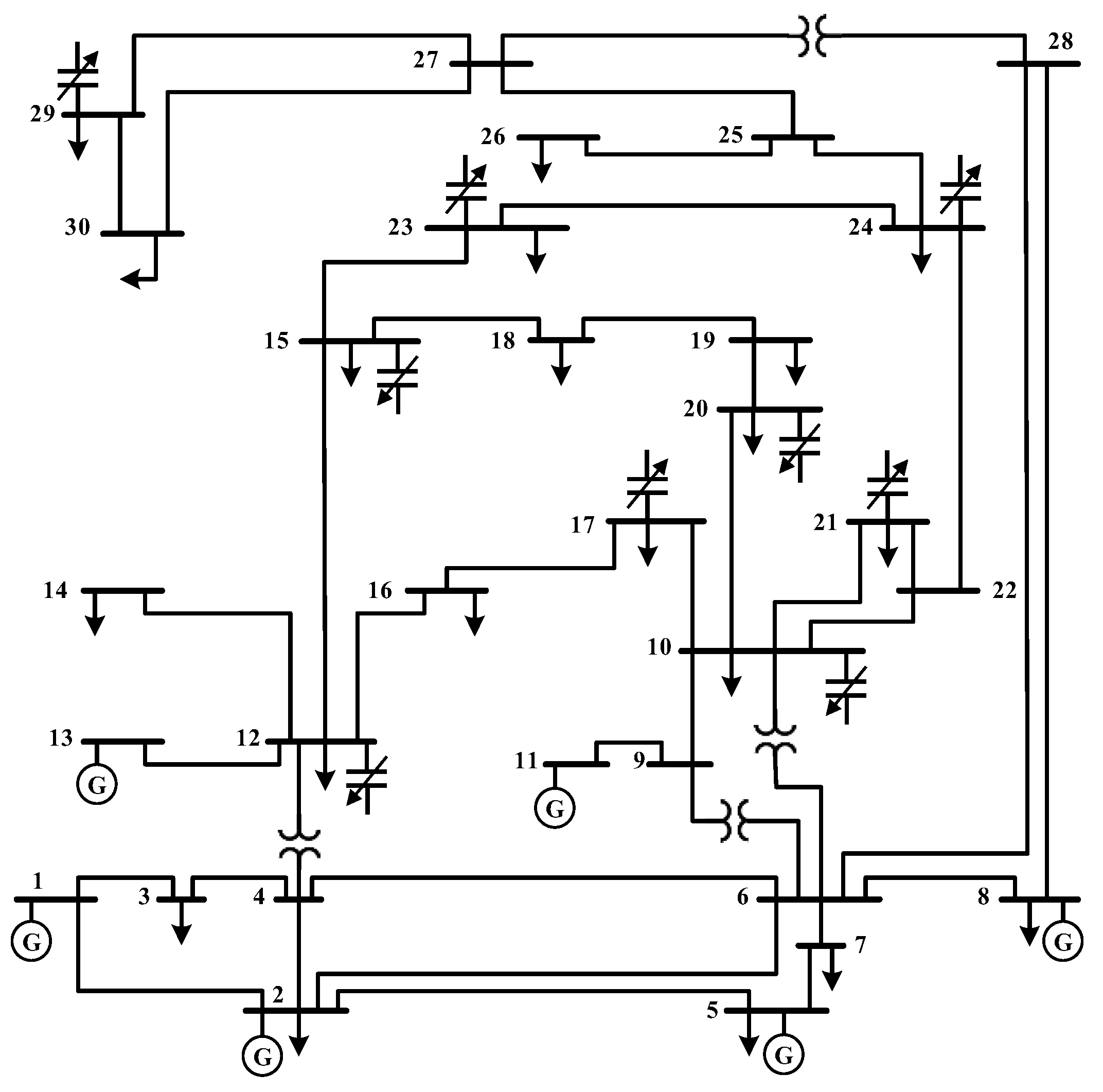
4.2. Obtained Results for the IEEE 30-Node System

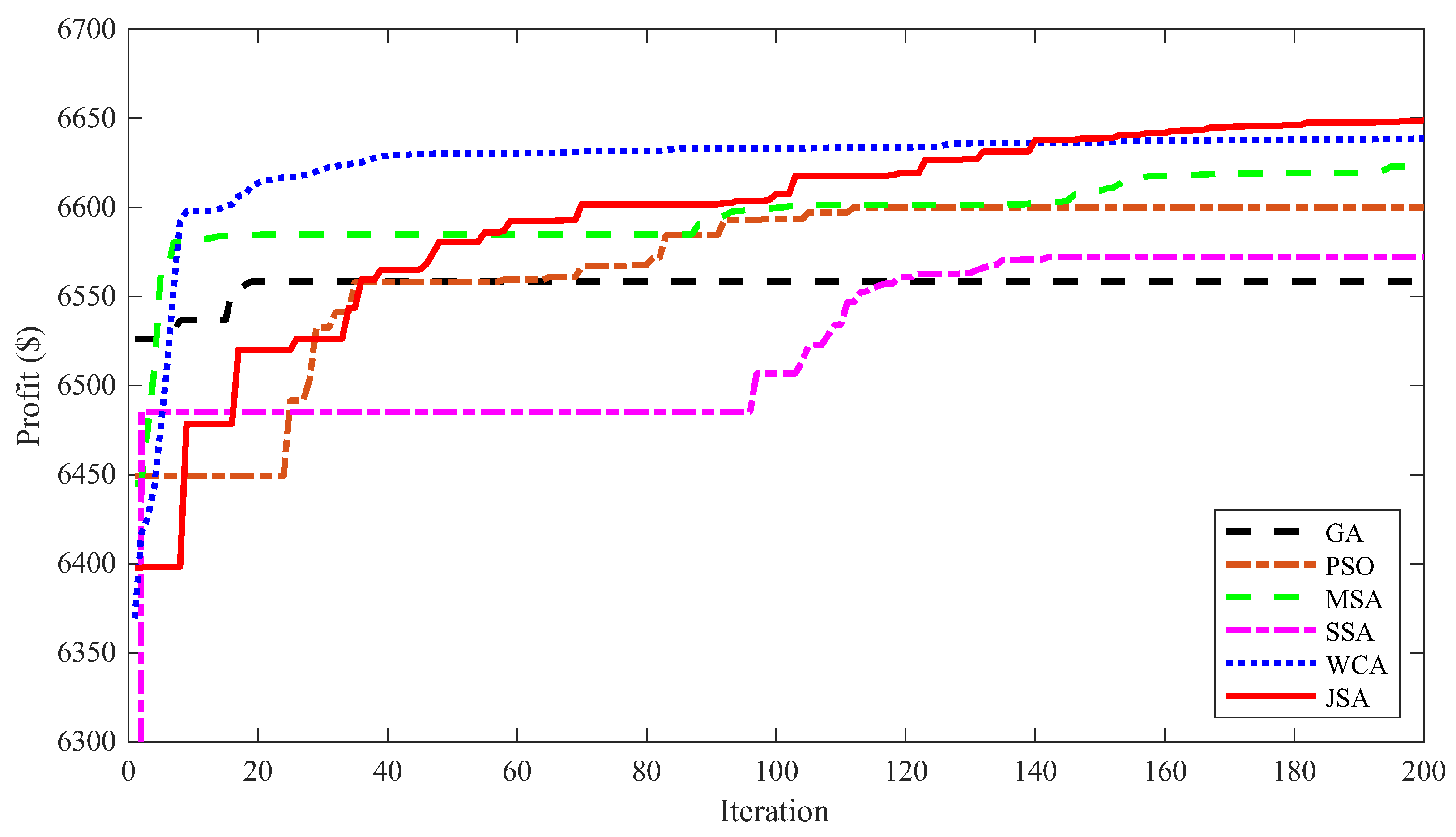
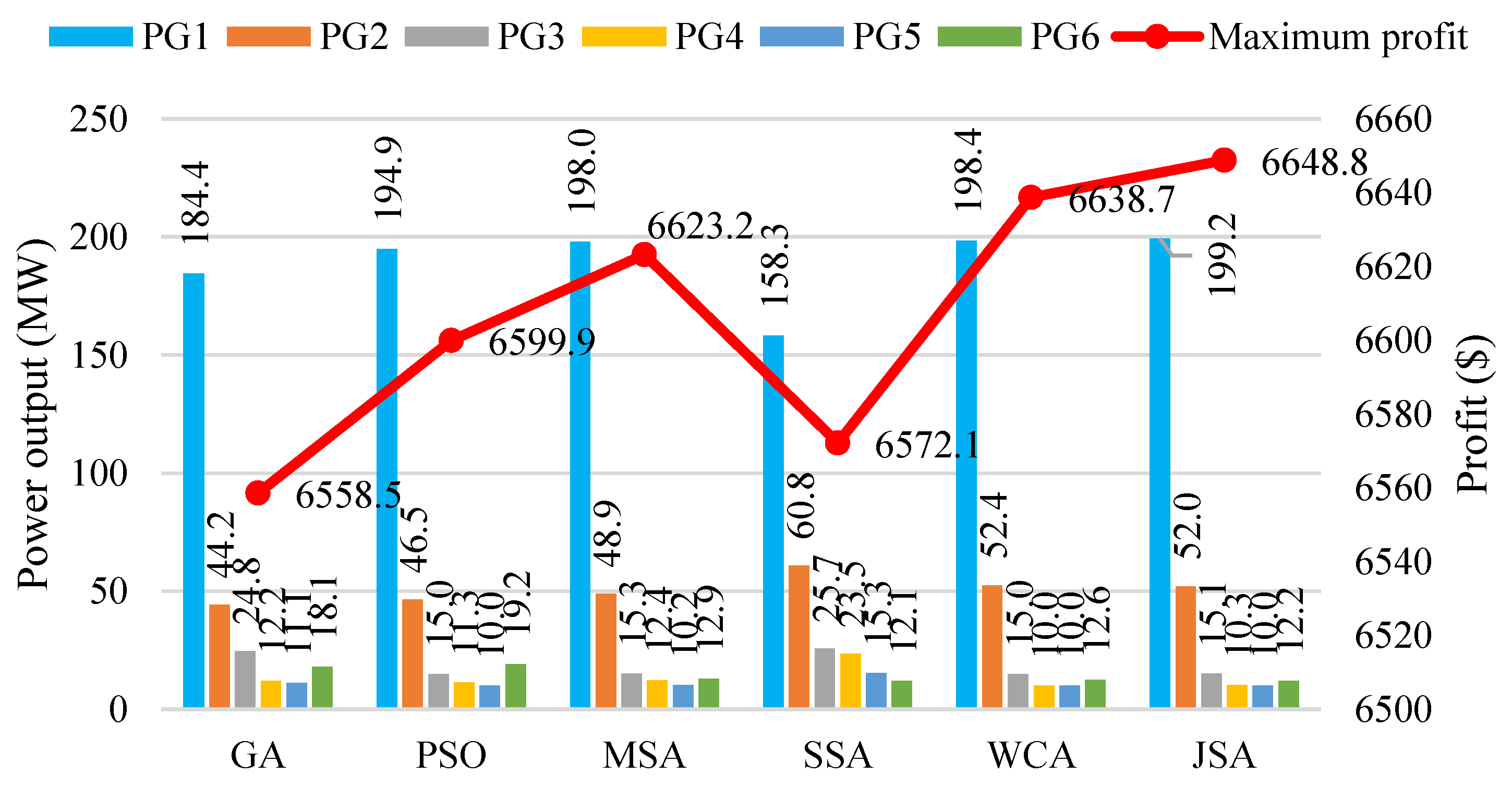
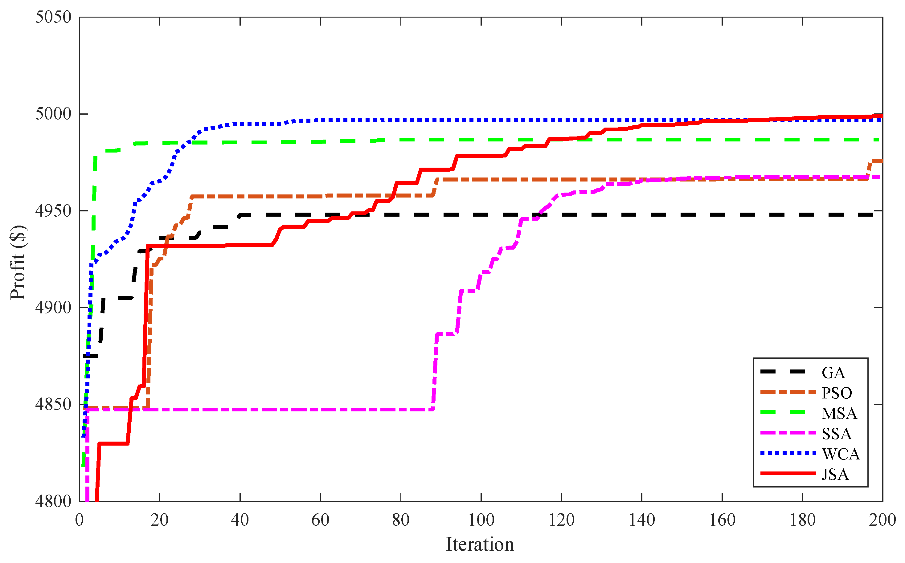
4.2.1. Results Obtained for Case 1

In Case 1, all applied algorithms are successful to reach valid solutions. One valid solution shows one profit value and fifty profit values for each algorithm are summarized in Figure 4. In the figure, six profit boxplots with different colors are plotted to compare the performance of algorithms. The box and whisker of JSA are shorter than those of five other ones. The upper extreme, the lower extreme, and the median of JSA are, respectively, higher than those of others to confirm that JSA can reach better maximum profit, better mean profit, and better minimum profit than others. Median of JSA is much higher than the upper quartile of others, and even the lower quartile of JSA is also higher than the upper quartile of MSA and SSA. Notice here the deviation between the median of JSA and the first quartile of others. The height of yellow box is smaller than other boxes, and the yellow whiskers are also shorter than other whiskers. Concerning a clear number for comparisons, JSA reaches more profit than MSA, SSA, WCA, PSO, and GA by 0.4%, 1.2%, 0.2%, 0.7%, and 0.75%, respectively. The special result here is that the minimum profit of JSA is $6610.7, but the maximum profit of SSA, PSO, and GA is $6572.1, $6599.9, and $6558.5. Additionally, the mean profit of JSA is $6629.1, but the maximum profit of MSA is $6623.2. The comparisons indicate the following remarks:
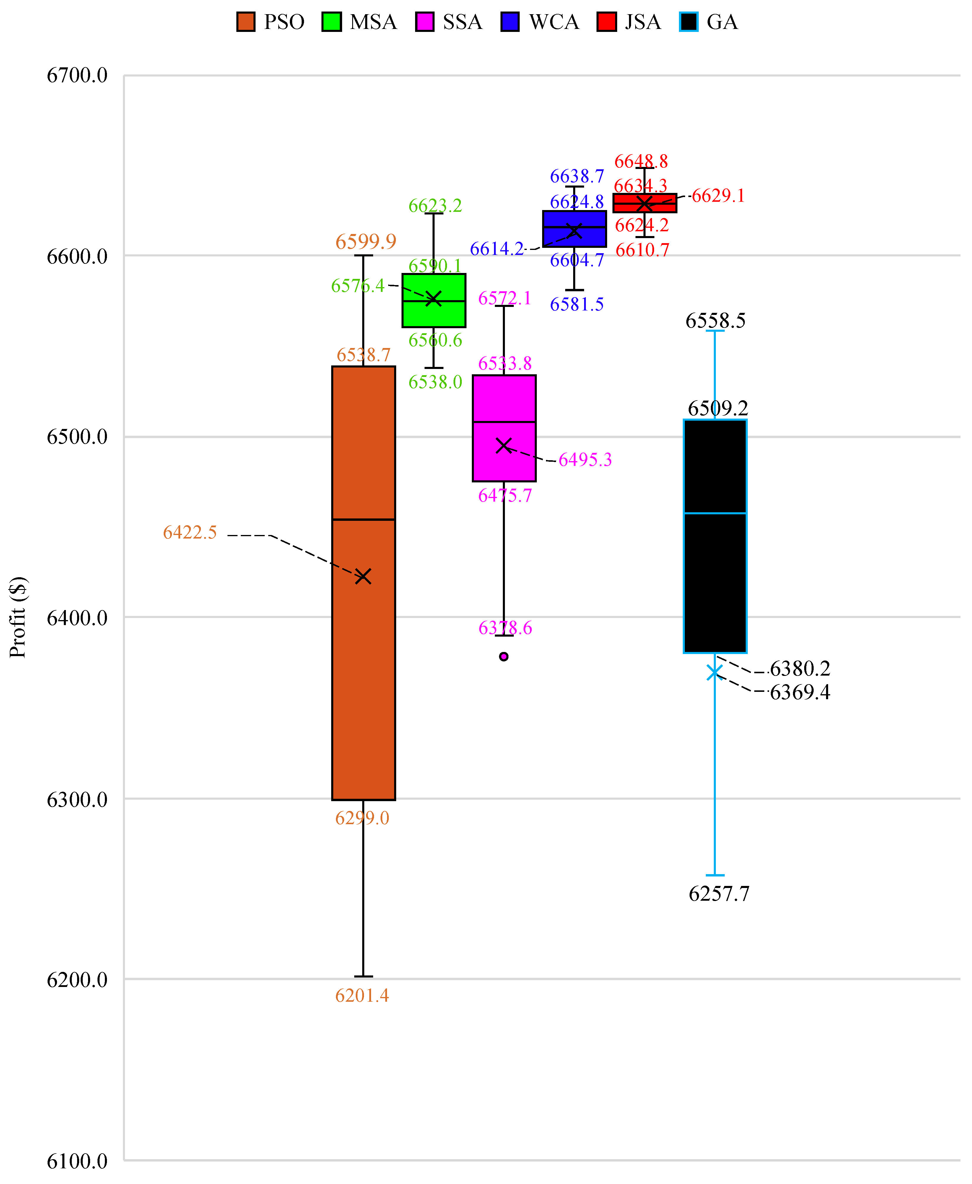
  • All solutions of JSA are much better than those of SSA, GA and PSO
  • Almost all solutions of JSA are better than those of MSA,
  • JSA has many better solutions than WCA.
Figure 5 presents the best run among the fifty trials reaching the maximum profit obtained by six applied algorithms. In the figure, JSA can reach greater profit than SSA (from the 18th iteration to the last iteration), MSA (from the 60th iteration to the last iteration), WCA (from the 140th iteration to the last iteration), PSO (from the 40th iteration to the last iteration), and GA (from the 40th iteration to the last iteration). On the other hand, the profit of JSA found at the 40th iteration, the 80th iteration, the 50th iteration, the 130th iteration, and the 160th iteration is, respectively, greater than the profit of GA, PSO, SSA, MSA, and WCA found at the last iteration (iteration 200). Clearly, JSA is much faster than others in searching for high-quality solutions.
Optimal power output of each thermal unit and total generation of all thermal units are given in Figure 6 and Figure 7, respectively. In general, JSA has different generation values with others for each thermal units. Additionally, the total generation of JSA is also different from that of others. The power loss of JSA is the same as WCA with 10 MW, whereas that of others is different. SSA has the smallest power loss, but it has not reached the best profit. The phenomenon is because of the ineffectiveness of other control parameters from SSA. It is recalled that a solution of optimal power flow is comprised of control variables and dependent variables, as shown in Section 3. Active power generation of thermal units is a part of control variables, and it cannot decide the quality of an obtained solution. So, SSA cannot reach the same good profit as others.

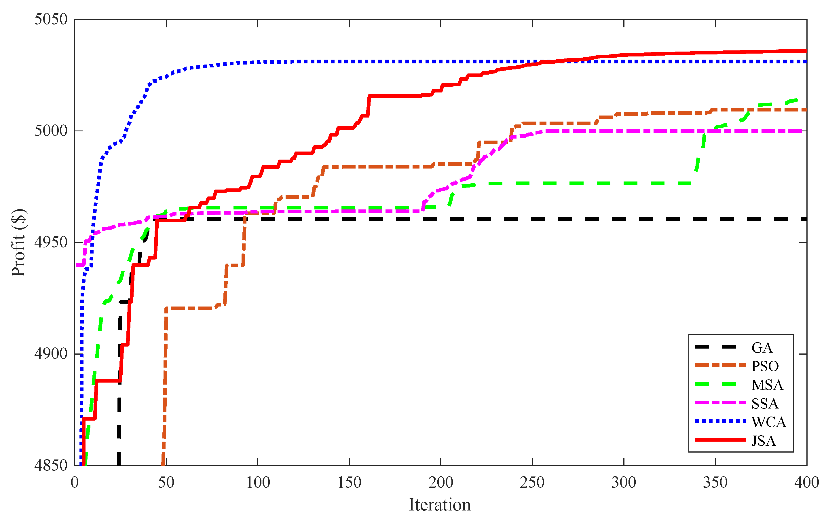
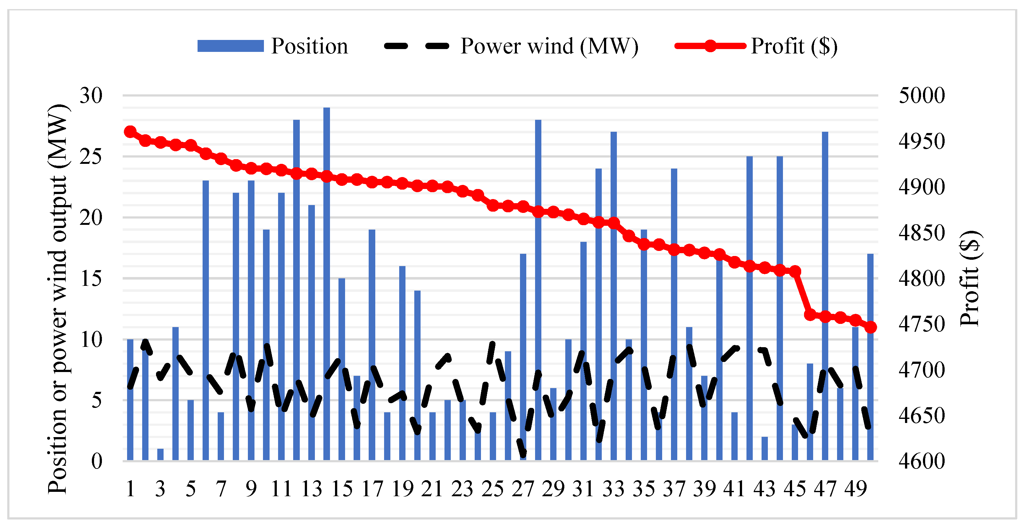
4.2.2. Results Obtained for Case 2 and Case 3

Results obtained by the six applied algorithms for Case 2 and Case 3 are reported in Figure 8 and Figure 9, respectively. The two figures have the same manner that the box and the whisker of JSA are the shorter than those from other algorithms and are located above those from others.
For Case 2, the maximum profit of JSA is $4998.8, while that from WCA, MSA, SSA, PSO, and GA is $4997.0, $4986.6, $4915.6, $4975.8, and $4948.0. JSA reaches greater maximum profit than WCA, MSA, SSA, PSO, and GA by $1.8, $12.2, $83.2, $23, and $50.8, respectively. The higher profit is equivalent to 0.04%, 2.44%, 1.7%, 0.46%, and 1.02% of the profit from these algorithms. Especially, the upper quartile of JSA is $4994.4. Meanwhile, that of these algorithms is, respectively, $4983.8, $4965.1, $4915.6, $4945.2, and $4948.0. The deviations indicate that the top solutions of JSA are more outstanding than others. Furthermore, the lower quartile of JSA is slightly smaller than the upper quartile of WCA and much higher than the upper quartile of others. This information indicates that the low-quality solution group of JSA is approximately equal to the top solutions of WCA and much better than the top solutions of MSA, SSA, PSO, and GA.
The summary of results in Figure 9 for Case 3 also indicates the best performance of JSA as compared to PSO, GA, MSA, SSA, and WCA. The best profit of JSA is greater than that of PSO, GA, MSA, SSA, and WCA by 1.2%, 1.52%, 0.4%, 1.3%, and 0.1%, respectively. In addition, other comparisons show the outstanding performance of JSA. In fact, the worst profit of JSA is $4990.3, which is much greater than the best profit of SSA, $4972.6. The upper extremes of PSO, GA, MSA, SSA, and WCA with $4975.8, $4960.5, $5014.2, $4972.5, and $5031.0 are smaller than the upper quartile of JSA with $5031.2. These comparisons indicate that JSA can reach more optimal solutions than others, and the number of high-quality solutions of JSA is also much greater than that of other. Thus, JSA is very effective for the study case of placing wind turbines in transmission power networks.
Figure 10 and Figure 11 present the best trial of algorithms over 50 independent trials for Case 2 and Case 3. The two figures have the same manner that WCA can reach greater profit than JSA from the first iteration to the 170th iteration for Case 2 and from the first iteration to about the 280th iteration for Case 3. For the last 30 iterations in Case 2 and the last 120 iterations, JSA can improve the profit more effectively than WCA. As compared to four remaining algorithms, JSA is much faster than them. Especially, JSA is about three times faster than PSO, SSA, and GA. For Case 2, the profit of JSA at the 100th iteration is much greater than that of the three algorithms at the last iteration (iteration 200). For Case 3, the profit of JSA at the 150th iteration is much greater than that of the three algorithms at the last iteration (iteration 400).
In summary, JSA is very effective for the OPF problem with the placement of wind turbine and nodal prices. So, we only implement JSA for other cases in the following section.
Figure 12, Figure 13, Figure 14, Figure 15, Figure 16 and Figure 17 report optimal location and optimal size of wind turbine together with profit of each run over 50 executed runs obtained by the six applied algorithms. To plot the figures, the fifty solutions were sorted from the greatest to the smallest, and then location and size corresponding to each solution were added together with its profit. As shown in Figure 12, the best location and the best size of wind turbine are, respectively, bus 5 and 10 MW. Similarly, the best factors of WCA, MSA, SSA, GA, and PSO are, respectively, bus 2 and 10 MW, bus 17 and 10 MW, bus 20 and 5 MW, bus 10 and 6 MW, and bus 7 and 10 MW, respectively. Clearly, 10 MW is the best size for the turbine and the three algorithms. JSA, WCA, MSA, and PSO have chosen it. However, the best location is bus 5, and only JSA could find it. On the other hand, JSA found many solutions with the same bus 5 and the same size 10 MW, while other algorithms could not reach the same performance. However, not every solution with the same bus 5 and size 10 MW can reach the same profit. Go back to the OPF problem. A solution of the original OPF problem without the placement of renewable energies is separated into control variables and dependent variables. The former set is comprised of active power generation of thermal units, excluding the unit at slack node, voltage of all thermal units, reactive power generation of capacitors, and tap changer value of transformers, whereas the later set is consisting of the generation of the unit at slack node, reactive power of all thermal units, voltage of all loads and apparent power of all transmission lines. Solutions could not reach the same control variable values, so the solutions had to have different dependent variables. As a result, although many solutions have the same bus 5 and the same size 10 MW for the added turbine, their profit was not the same as the best solution.

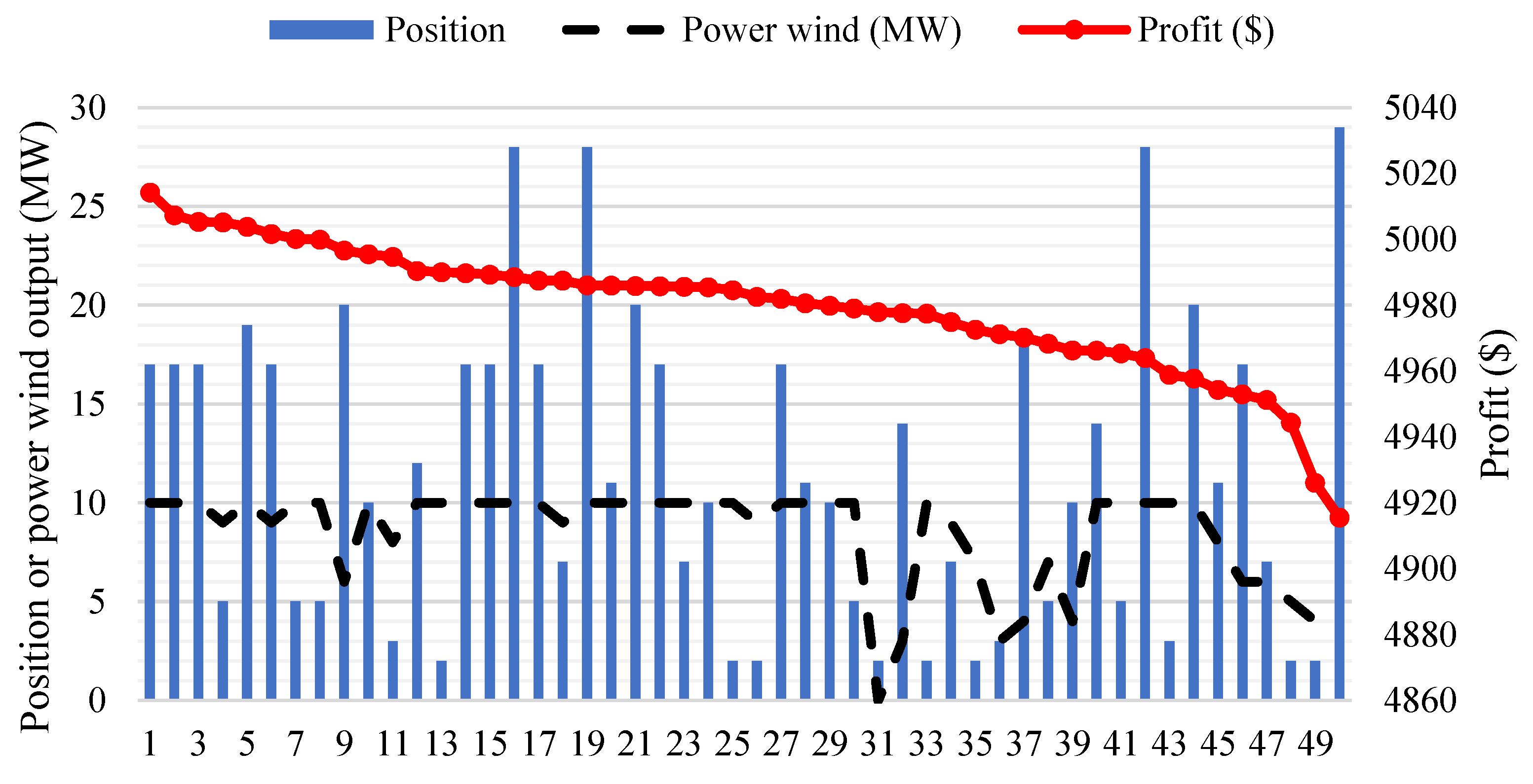
4.2.3. Results Obtained for Case 4

For finding the best solution of using wind turbine in the IEEE 30-node system, Case 4 has been implemented by using only JSA and applying the best location bus 5 and the best size 10 MW. JSA with the best performance has been run 50 times for reaching other parameters of the transmission network. As a result, fifty optimal solutions collected for determining profit values and summary of profits consist of the best, mean, and worst profits with $5035.9, $5026.0, and $4997.3, respectively. The results of Case 4 are compared to those from Case 3, as shown in Figure 18. In general, all profits of Case 4 are slightly greater than those of Case 3. Namely, Case 4 reaches greater maximum, mean, and minimum profits than Case 3 by $0.1, $2.3, and $7.0, respectively.
It is recalled that Case 3 optimizes location of wind turbine, rated power of the wind turbine, and all parameters of transmission power network. However, Case 4 uses the predetermined location and predetermined rated power of Case 3 and only optimizes all parameters of transmission power network. So, the small profit deviation between Case 3 and Case 4 indicates that JSA is very effective for a complicated OPF problem with renewable energy.

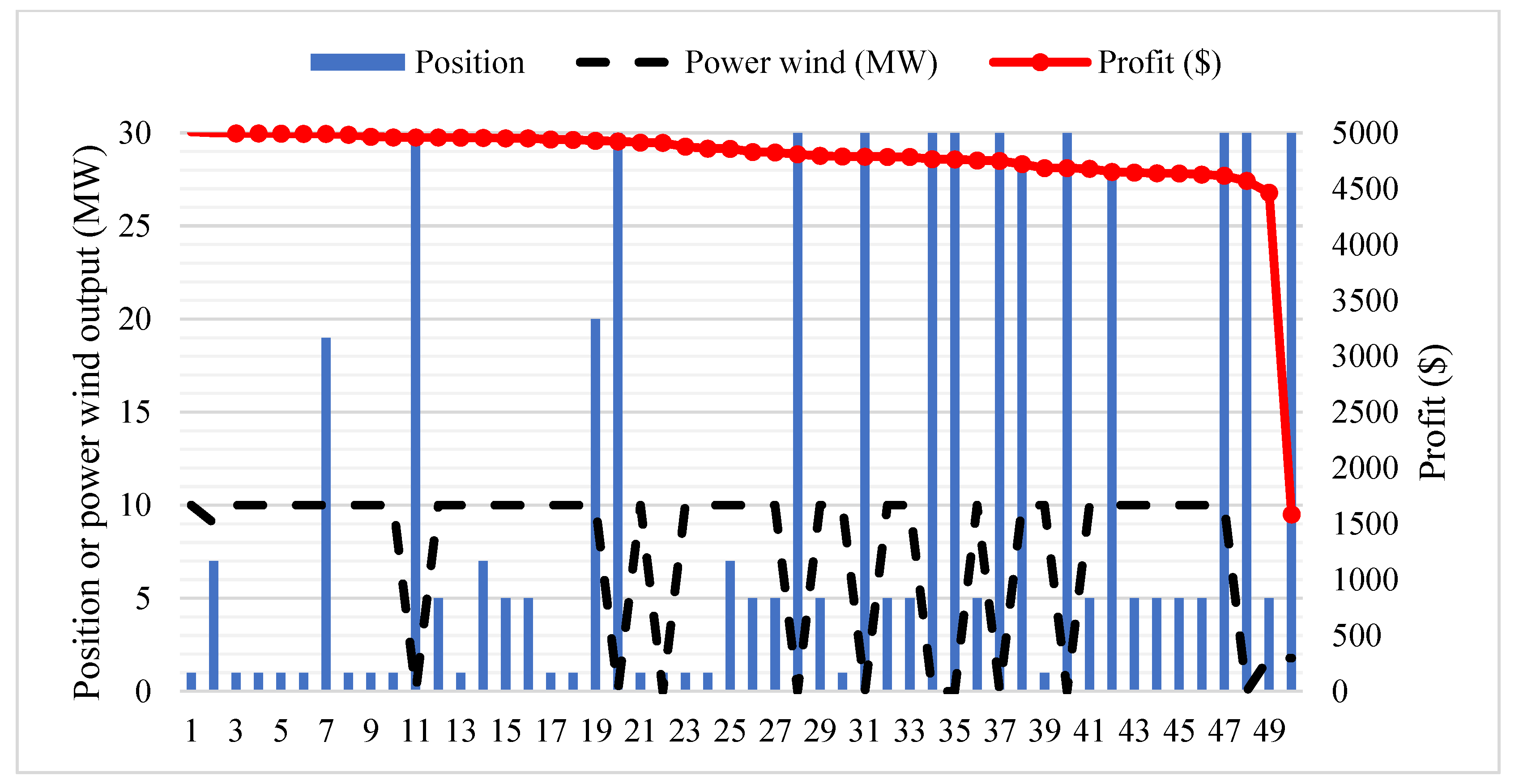
4.2.4. Results Obtained for Case 5

In this section, JSA is implemented for determining optimal location and optimal size of three subcase—5.1, 5.2, and 5.3 with 2, 3, and 4 wind turbines, respectively. The optimal solution of the study cases, together with that of Case 2 and Case 3, are reported in Table 3. We can see that Node 5 is selected for all study cases. For using at least two WTs, Node 2 is always selected. Node 1 is selected for two Cases, with 3 and 4 WTs, while Node 10 is selected for the last case with 4 WTs. Clearly, Node 5 is the most prior location and Node 10 is the least prior location for installing a wind turbine with 10 MW. In summary, the important order for installing WTs is Node 5, Node 2, Node 1, and Node 10. With respect to the power, all wind turbines are suggested to be 10 MW.
Figure 19 shows maximum profits of these study cases. As using more wind turbines, the maximum profit is higher. Case 3 with one wind turbine has more profit than Case 2 without wind turbine by $37. The profit of two WTs is $5093.7, which is more than the profit of one WT, $5035.8 by $57.8. Similarly, three WTs can reach greater profit than two WTs by $9.2, and four WTs can reach greater profit than three WTs by $26.2. The comparisons indicate that the placement of two wind turbines is the most effective and locations at node 5 and node 2 are the best for placing wind turbines. On the other hand, the use of four WT can reach greater profit than base system by $130.3, which is equivalent to 2.6% of the base system. The profit improvement is not much, and it is also a problem to consider if the four WTs should be placed in the system for the purpose of benefit.
Optimal control variable of wind turbines and optimal control variables of the IEEE 30-node system for different cases are reported in Table A3 in Appendix A.

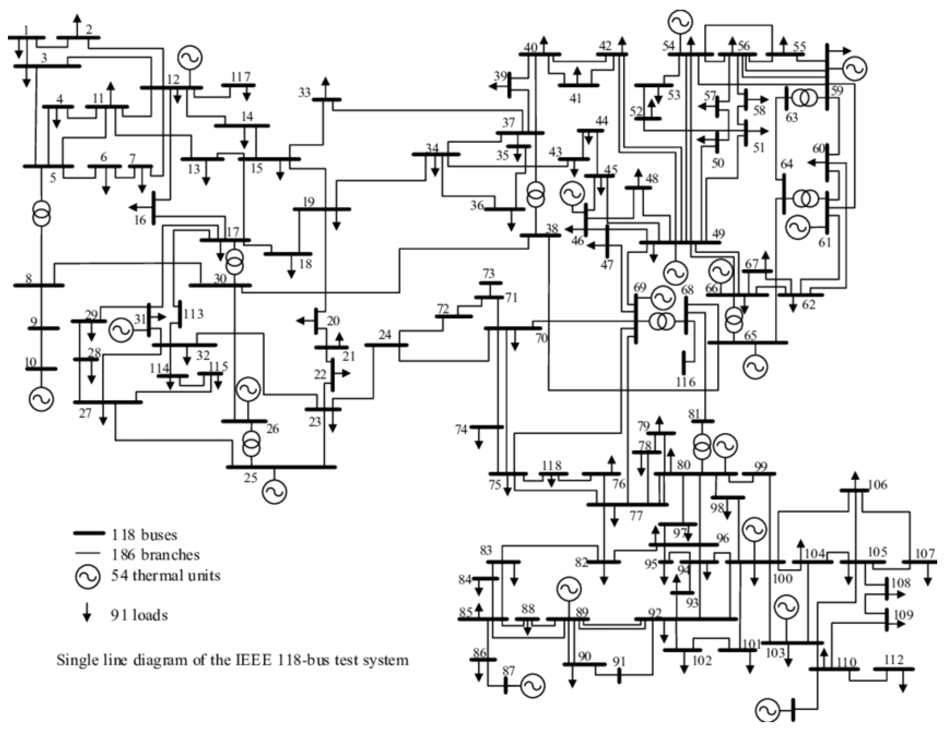
4.3. Obtained Results for the IEEE 118-Node System

In this section, only JSA is run for the IEEE 118-node system for reaching the best profit of different number of wind farms. Each wind farm is supposed to be from 0 MW to 100 MW. The first duty of JSA is to find both location and size of each wind farm. In the second duty, JSA must find all control parameters of the IEEE 118-node system, as shown in Section 3. The solutions of wind farms placement are given in Table 4. Meanwhile, the profit of each case is given in Figure 20. Table 4 can see the important order of nodes for placing wind farms. The order of nodes arranged from the most to the least importance is nodes 29, 31, 71, 45 and 47.
As shown in Figure 20, the profit is increased as the number of wind farms is increased. The lowest profit of $35,777.8 and the highest profit of $70,548.2 are obtained for the cases without wind farms and with five wind farms. Five wind farms can help the system reach greater than the base system without wind farms by $34,770.4. This greater profit is equivalent to 97.2% of the base system. So, the contribution of JSA for improving profit is significant.
On the other hand, the increase in profit as using higher number of wind farms is also seen clearly in Figure 20. One wind farm can reach higher profit than without wind farm by $10,620.9, equivalent to 29.69%. Similarly, two wind farms can reach greater profit than one wind farm $9553.9, equivalent to 20.59%. Other comparisons also indicate the same manner, but the values are smaller. The greater profits are, respectively, $4574.6, $5076, and $4944.9, equivalent to 8.18%, 8.39%, and 7.54%. The smaller percent values can reveal the greater profit is proportional to the number of wind farms. The most effective number of wind farms can be two wind farms. However, the wind power cost is free due to the availability of wind speed. So, more wind power generated can lead to higher benefit if the initial investment cost is neglectable. In fact, the initial investment cost for installing wind farms is very high. Meanwhile, the fuel cost of wind farms is zero. This characteristic is opposite to thermal power plants, with not very high investment cost, but with very high cost of fossil fuels. The power system with 118 nodes has 54 thermal units, and all loads are supplied by the power sources. If the fossil fuel is not enough to run generating units, demand of loads must be cut intentionally. So, the investment of wind farms is essential.

5. Conclusions

This paper has studied optimal power flow for the IEEE 30-node and 118-node transmission power networks considering electric market and renewable energies, namely, nodal prices and wind turbine placement. Electricity prices at different nodes were given by different values. Meanwhile, wind turbines in the range from 0 MW to 10 MW for the first system and wind farms from 0 to 100 MW for the second system were placed at different nodes. For the first system, three cases, including (1) the same prices for all nodes, (2) different prices for different nodes, and (3) different prices for different nodes and the placement of one wind turbine, were implemented by using six applied algorithms, PSO, GA, MSA, SSA, WCA, and JSA. The results from the three cases are summarized as follows:
  • For Case 1, JSA obtained greater profit than MSA, SSA, WCA, PSO, and GA by 0.4%, 1.2%, 0.2%, 0.7%, and 0.75%, respectively. For Case 2 and Case 3, these values are 0.04%, 2.44%, 1.7%, 0.46%, and 1.02% and 1.2%, 1.52%, 0.4%, 1.3%, and 0.1%, respectively.
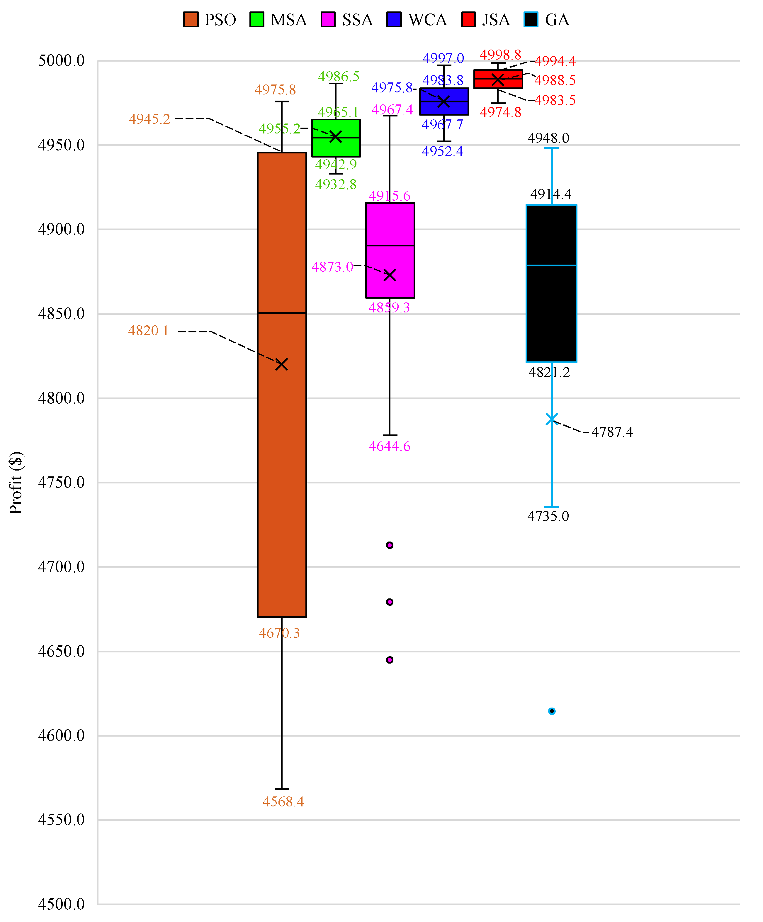
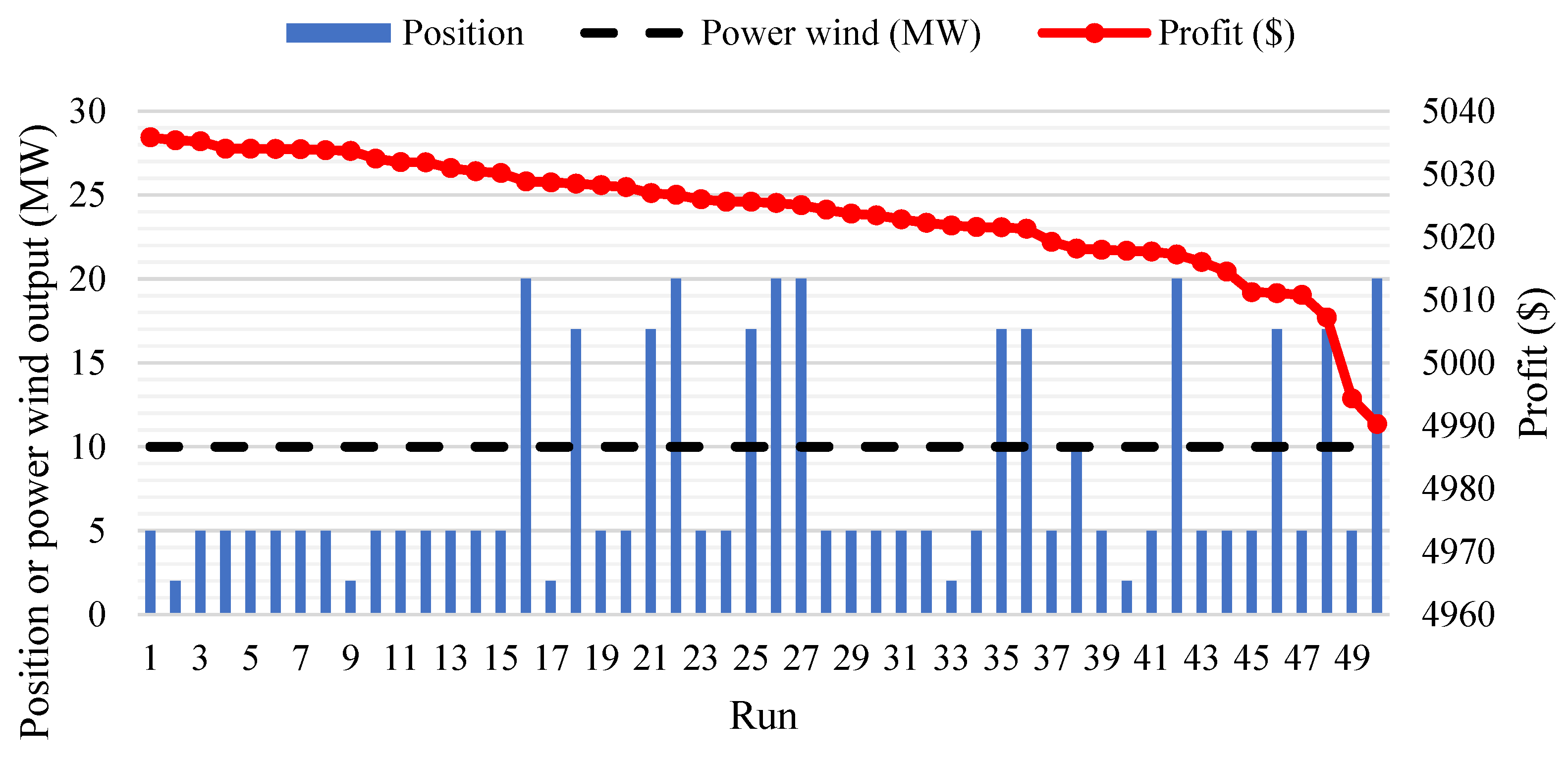
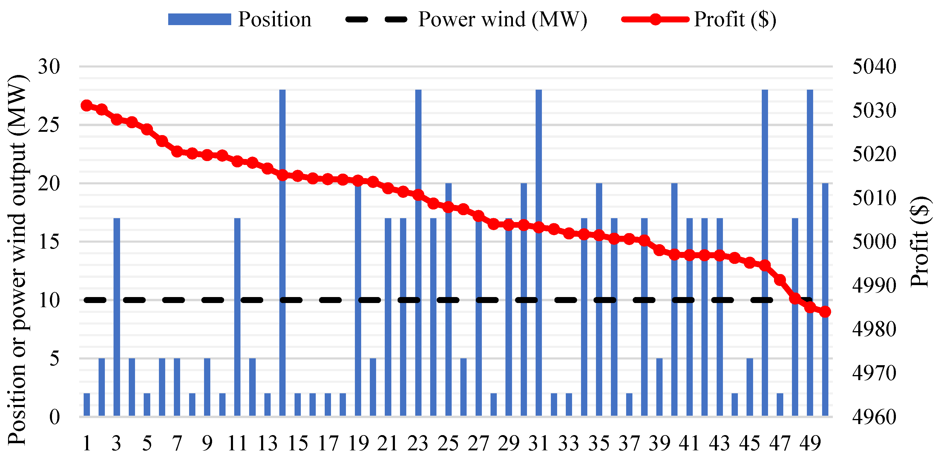
  • Approximately all fifty solutions of JSA had a small deviation of profit, and its number of high-quality solutions was high. However, five remaining algorithms had big deviation and a small number of good solutions.
  • JSA is much faster than others at least two times. The final solution of others at the last iteration was worse than a solution of JSA at a half iteration number.
The results above indicates that JSA is more effective than PSO, GA, MSA, SSA, and WCA in finding the best solutions for OPF problem considering electric market and renewable energy. Thus, JSA has been selected to implement Case 4 and Case 5 of the first system and six other cases of the second system. For the first system, Case 4 used the optimal location and rated power of the added wind turbine in Case 3 to optimize all parameters of transmission power network. Case 5 optimized the placement of two, three, and four wind turbines in three subcases 5.1, 5.2, and 5.3. For the second system, JSA has been run for optimizing zero, one, two, three, four, and five wind farms. The results and indications are as follows:
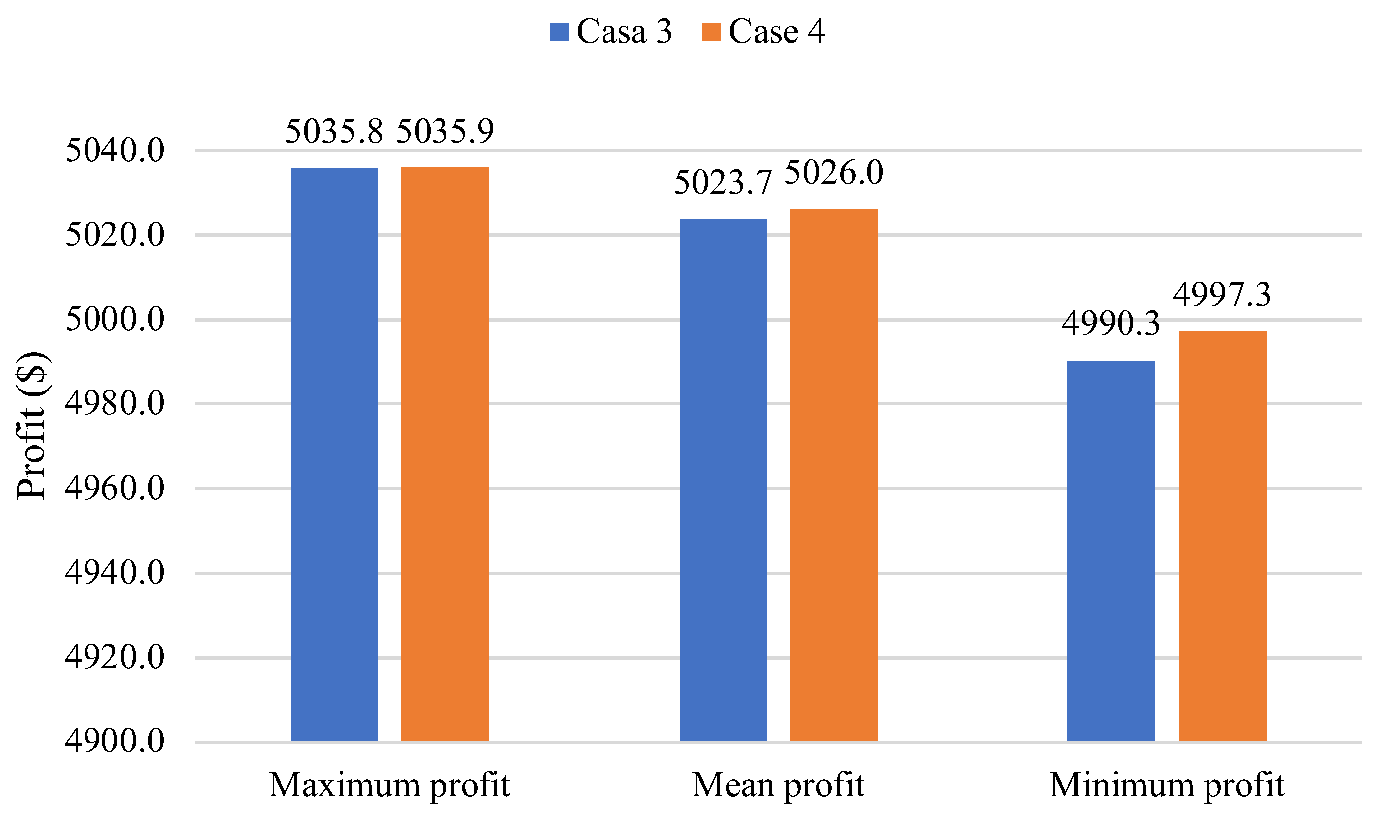
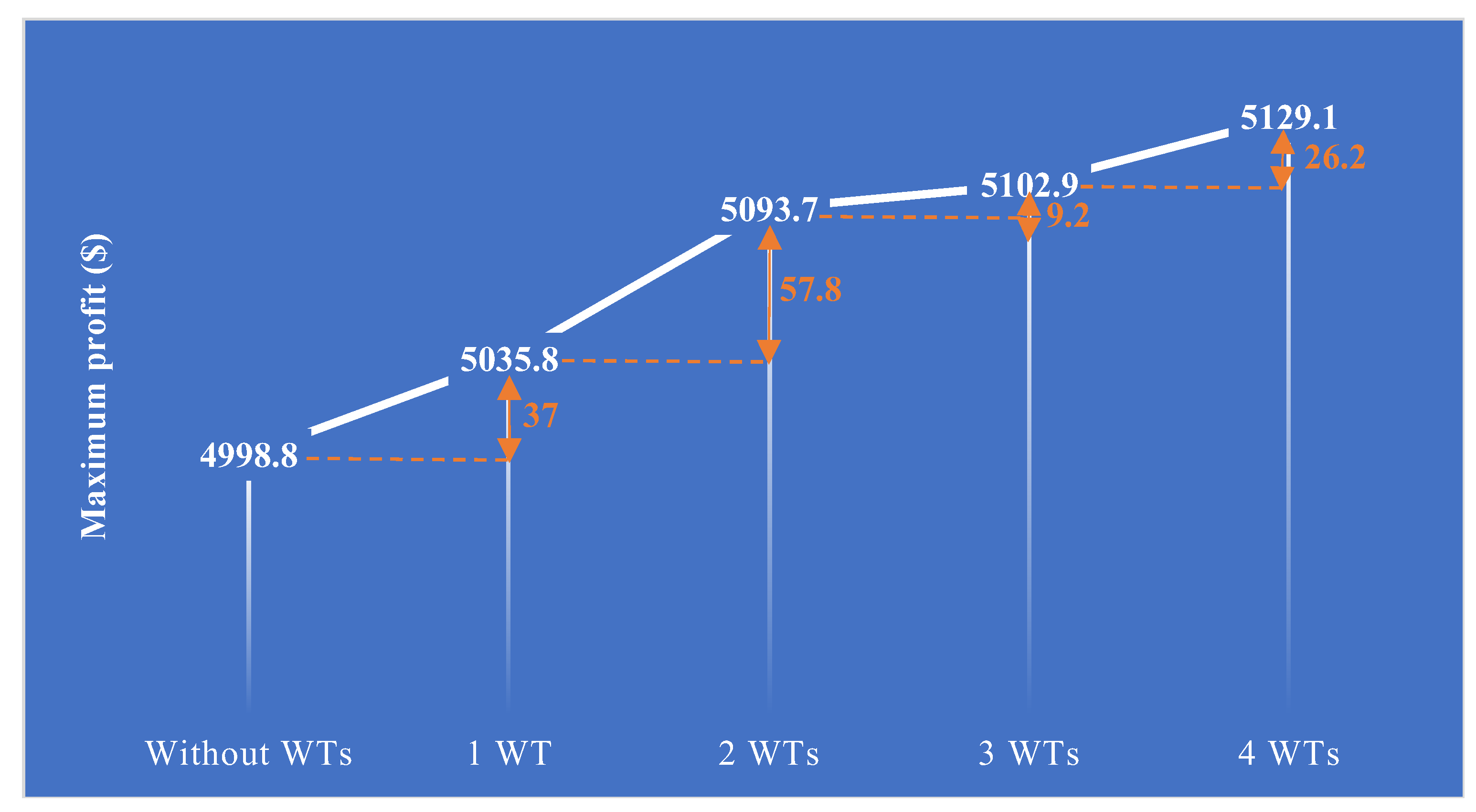
  • For the first system, JSA had approximately the same profit for Case 3 and Case 4, although Case 3 was more complicated. Case 3 optimized two factors of wind turbine and all parameters of transmission power network, but only all parameters of transmission network were optimized in Case 4. This result indicated that JSA was very effective for the complex problem with transmission network and renewable power plants. Three subcases in Case 5 indicated that higher profits could be reached when more wind turbines were placed. The effectiveness order of nodes for placing wind turbines was Node 5, Node 2, Node 1, and Node 10.
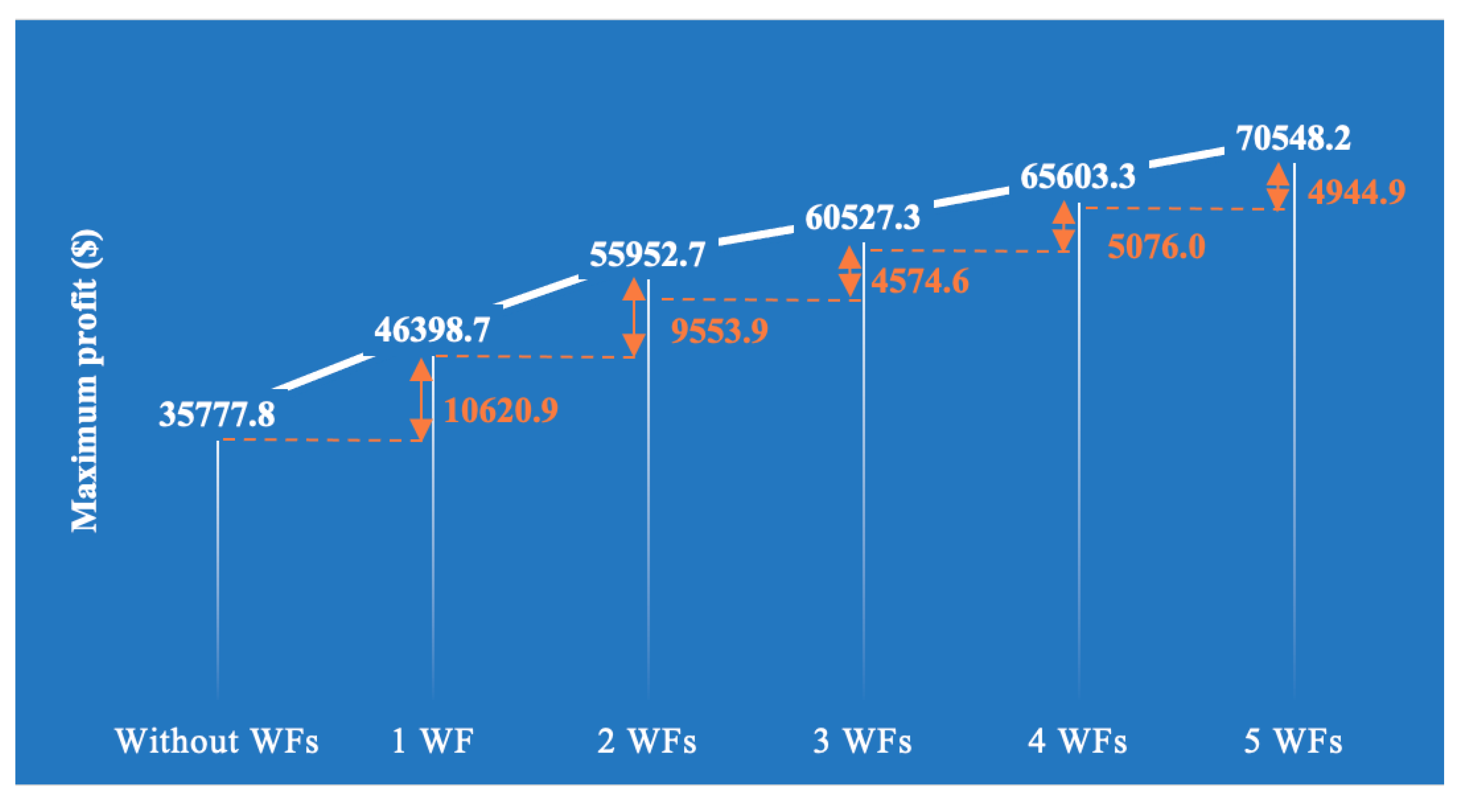
  • For the second system, the order of nodes arranged from the most to the least importance is nodes 29, 31, 71, 45, and 47. As following the order, the profit can be reached effectively. In fact, the system with one wind farm can reach higher profit than the base system without wind farm by 29.69%. When increasing the wind farms to two, three, four, and five, the profit is greater by 20.59%, 8.18%, 8.39%, and 7.54%. Clearly, the important nodes have high impact on the increase in profit. On the other hand, the system with five wind farms can reach greater than the base system by 97.2%.
Clearly, the contributions of the study are significant in reaching high profit for the two transmission power networks and suggesting the number of wind turbines, the location, and size of each wind turbine for reaching the highest profit. In addition, JSA was the most effective algorithms that could be believed for OPF problem. However, the study also has shortcomings. The study neglected the real wind speeds at each location in two power systems, and the change in load within one day or one year was not considered. The operation schedule with one day (twenty-four hours) or one year (twelve months with average load and average solar radiation and average wind speed over twenty-four hour per day) can be considered for future work. Both solar power and wind power with the consideration of uncertain solar radiation and uncertain wind speed are hot topics for the future work, too.

Author Contributions

Writing – original draft, T.T.N.; Writing – review & editing, H.D.N. and M.Q.D.; Supervision, M.Q.D. All authors have read and agreed to the published version of the manuscript.

Funding

This research received no external funding.

Institutional Review Board Statement

Not applicable.

Informed Consent Statement

Not applicable.

Data Availability Statement

Not applicable.

Acknowledgments

We acknowledge Ho Chi Minh City University of Technology (HCMUT), VNU-HCM for supporting this study.

Conflicts of Interest

The authors declare no conflict of interest.

Abbreviations

OPFOptimal Power Flow
WFsWind farms
PVSsSolar photovoltaic systems
JSAJellyfish search algorithm
MSAMoth swarm algorithm
SSASalp swarm algorithm
WCAWater cycle algorithm
PSOParticle swarm optimization
GAGenetic algorithm
Nomenclature
S y s P r o f i t Profit of the considered system
T o R e E l e c The total revenue of electricity sale
C o s t F u e l The total fuel cost of all thermal units in the transmission power networks
c e 1 k ,   c e 2 k ,   c e 3 k Given coefficients in fuel cost function of the kth thermal unit
N T U s Thermal unit number
N L o a d s Load number
E P r l Electricity price ($/MWh) at the lth load
P L o a d l Load demand at the lth load node
N W P s Number of wind turbines installed in the system
PWm, QWmActive and reactive power generation of the mth wind turbine
Q T k Reactive power generation of the kth thermal unit
N B r s Number of transmission lines
P L o s s , b , Q L o s s , b Active and reactive power loss on the bth transmission lines
Q C c Reactive power generation of the cth capacitor
N C a p s Number of capacitors
Q L o a d l Reactive power demand of load at the lth load node
P T i   ,   P W i   , P L o a d i Active power generation of thermal unit and wind tubines at the ith node
V o l i , V o l j Voltages of the ith and jth buses
B S i j , G C i j Transfer susceptance and the conductance between the ith node and the jth node
N n o d e s Number of nodes
θ j and θ i Angles of voltage at the jth node and the ith node, respectively
Q C i M i n , Q C i M a x The lowest and highest generation of the capacitors at the ith node
P T k M i n ,   P T k M a x The smallest and highest active power generations of the kth thermal unit
Q T k M i n ,   Q T k M a x The smallest and highest reactive power generations of the kth thermal unit
P W m   M i n ,   P W m   M a x The smallest and highest active power generations of the mth wind turbine
Q W m   M i n ,   Q W m   M a x The smallest and highest reactive power generations of the mth wind turbines
  T p n   Tap value of the nth transformer
T p M i n ,   T p M a x The smallest and highest tap values of all transformers
N TF Number of used transformers
d r 1 , d r 2 , d r 3 Random numbers within 0 and 1
S N * , S N m i d The best and mean solutions of the current population
S N r d A random solution in the present population
F i t r d , F i t j Fitness values of two solutions, S N r d and S N j
L W P m , PF W P m Location and power factor of the mth wind farm
S N j M i n , S N j M a x Lower and upper boundaries of the solution S N j
D S j The jth dependent variable set
D S j M i n , D S j M a x Lower and upper boundaries of the jth dependent variable set
F i t j n e w Fitness value of the new solution jth

Appendix A

Table A1. Nodal prices of the IEEE 30-node system.
NodePrice ($/MWh)NodePrice ($/MWh)
119.541619.7
219.621720.03
319.521819.94
419.511920.16
520.952020.16
619.722119.67
720.32219.47
819.842318.88
919.922418.57
1020.022516.09
1119.912615.29
1219.152715.1
1315.22819.74
1419.432915.49
1519.383015.75
Table A2. Nodal prices of the IEEE 118-node system.
NodePrice ($/MWh)NodePrice ($/MWh)NodePrice ($/MWh)NodePrice ($/MWh)
148.55131100.3676135.3879148.574
250.5743248.7066248.3399248.204
352.6813350.3546333.5829350.212
448.3693448.5686436.8629434.725
550.3843550.6256533.7589536.114
648.2063648.4796631.6679636.114
750.2153750.5926732.9879734.607
848.0073850.5536835.1649834.725
932.3003950.5536933.2499948.504
1031.0084048.5317048.55710033.336
1137.1014150.9507150.45310152.221
1235.6174248.9127248.09410250.212
1350.3544350.5927348.43510334.349
1450.3544452.6167448.24310448.046
1548.3404557.5937550.25310548.208
1637.1014655.2907648.38010650.100
1750.5544757.5937748.53810748.096
1848.5324857.5937850.56110850.216
1948.3914931.7197934.60710950.074
2050.4085033.0408033.22211048.071
2152.4245133.0408134.60711131.143
2252.4245239.6158250.56111248.519
2350.4265338.0918352.00111348.676
2448.4095436.5688450.00111450.736
2529.1775548.7388548.00111550.608
2630.8715648.6008638.90311648.138
2748.5845750.6258737.34711737.101
2850.6085850.6258832.75211850.396
29104.5495932.2388931.442
3050.0076033.5829048.613
Table A3. Optimal solutions obtained by JSA for study cases with the placement of wind turbines and the consideration of electric market.
VariableCase 3Subcase 5.1Subcase 5.2Subcase 5.3
PT2 (MW)44.4444.2836.8231.54
PT5 (MW)20.5120.4017.7317.13
PT8 (MW)10.0310.0010.0010.00
PT11 (MW)10.0310.0010.0010.00
PT13 (MW)12.0012.0012.0012.00
Vol1 (Pu)1.101.101.101.10
Vol2 (Pu)1.061.061.061.06
Vol5 (Pu)0.950.950.950.95
Vol8 (Pu)0.950.950.950.95
Vol11 (Pu)0.970.970.970.97
Vol13 (Pu)0.980.980.980.97
QC10 (MVAr)0.070.000.000.00
QC12 (MVAr)0.285.005.000.11
QC15 (MVAr)0.230.000.000.00
QC17 (MVAr)0.180.000.000.00
QC20 (MVAr)1.741.341.343.72
QC21 (MVAr)0.070.000.000.00
QC23 (MVAr)0.100.000.000.00
QC24 (MVAr)0.000.000.000.00
QC29 (MVAr)1.165.005.005.00
Tp11 (Pu)0.900.900.900.90
Tp12 (Pu)1.071.101.101.10
Tp15 (Pu)0.900.900.900.90
Tp36 (Pu)0.900.900.900.90

References

  1. Nguyen, K.; Fujita, G. Self-Learning Cuckoo search algorithm for optimal power flow considering tie-line constraints in large-scale systems. GMSARN Int. J. 2018, 12, 118–126. [Google Scholar]
  2. Warid, W.A. Novel Chaotic Rao-2 Algorithm for Optimal Power Flow Solution. Int. J. Electr. Comput. Eng. 2022, 2022, 7694026. [Google Scholar] [CrossRef]
  3. Sulaiman, M.H.; Mustaffa, Z.; Mohamad, A.J.; Saari, M.M.; Mohamed, M.R. Optimal power flow with stochastic solar power using barnacles mating optimizer. Int. Trans. Electr. Energy Syst. 2021, 31, e12858. [Google Scholar] [CrossRef]
  4. Nguyen, T.T. A high performance social spider optimization algorithm for optimal power flow solution with single objective optimization. Energy 2019, 171, 218–240. [Google Scholar] [CrossRef]
  5. Shaqsi, A.Z.A.; Sopian, K.; Al-Hinai, A. Review of energy storage services, applications, limitations, and benefits. Energy Rep. 2020, 6, 288–306. [Google Scholar] [CrossRef]
  6. Pham, L.H.; Dinh, B.H.; Nguyen, T.T.; Phan, V.D. Optimal operation of wind-hydrothermal systems considering certainty and uncertainty of wind. Alex. Eng. J. 2021, 60, 5431–5461. [Google Scholar] [CrossRef]
  7. Gan, L.; Low, S.H. An online gradient algorithm for optimal power flow on radial networks. IEEE J. Sel. Areas Commun. 2016, 34, 625–638. [Google Scholar] [CrossRef]
  8. Bose, S.; Gayme, D.F.; Chandy, K.M.; Low, S.H. Quadratically constrained quadratic programs on acyclic graphs with application to power flow. IEEE Trans. Control Netw. Syst. 2015, 23, 278–287. [Google Scholar] [CrossRef] [Green Version]
  9. Tostado, M.; Kamel, S.; Jurado, F. Developed Newton-Raphson based predictor-corrector load flow approach with high convergence rate. Int. J. Electr. Power Energy Syst. 2019, 105, 785–792. [Google Scholar] [CrossRef]
  10. Fortenbacher, P.; Demiray, T. Linear/quadratic programming-based optimal power flow using linear power flow and absolute loss approximations. Int. J. Electr. Power Energy Syst. 2019, 107, 680–689. [Google Scholar] [CrossRef] [Green Version]
  11. Momoh, J.A. Electric Power System Applications of Optimization; CRC Press: Boca Raton, FL, USA, 2017. [Google Scholar]
  12. Hamza, M.F.; Yap, H.J.; Choudhury, I.A. Recent advances on the use of meta-heuristic optimization algorithms to optimize the type-2 fuzzy logic systems in intelligent control. Neural. Comput. Appl. 2017, 28, 979–999. [Google Scholar] [CrossRef]
  13. Abd El-sattar, S.; Kamel, S.; Tostado, M.; Jurado, F. Lightning attachment optimization technique for solving optimal power flow problem. In Proceedings of the 2018 Twentieth International Middle East Power Systems Conference, Cairo, Egypt, 18–20 December 2018; IEEE: New York, NY, USA, 2018; pp. 930–935. [Google Scholar]
  14. Berrouk, F.; Bounaya, K. Optimal power flow for multi-FACTS power system using hybrid PSO-PS algorithms. J. Control Autom. Electr. Syst. 2018, 29, 177–191. [Google Scholar] [CrossRef]
  15. Marcelino, C.G.; Almeida, E.; Wanner, E.F.; Baumann, M.; Weil, M.; Carvalho, L.M.; Miranda, V. Solving security constrained optimal power flow problems: A hybrid evolutionary approach. Appl. Intell. 2018, 48, 3672–3690. [Google Scholar] [CrossRef] [Green Version]
  16. Biswas, P.P.; Suganthan, N.; Mallipeddi, R.; Amaratunga, G.A. Optimal power flow solutions using differential evolution algorithm integrated with effective constraint handling techniques. Eng. Appl. Artif. Intell. 2018, 68, 81–100. [Google Scholar] [CrossRef]
  17. Kahraman, H.T.; Akbel, M.; Duman, S. Optimization of optimal power flow problem using multi-objective manta ray foraging optimizer. Appl. Soft Comput. 2022, 116, 108334. [Google Scholar] [CrossRef]
  18. Nadimi-Shahraki, M.H.; Fatahi, A.; Zamani, H.; Mirjalili, S.; Oliva, D. Hybridizing of Whale and Moth-Flame Optimization Algorithms to Solve Diverse Scales of Optimal Power Flow Problem. Electronics 2022, 11, 831. [Google Scholar] [CrossRef]
  19. Akdag, O. An improved archimedes optimization algorithm for multi/single-objective optimal power flow. Electr. Power Syst. Res. 2022, 206, 107796. [Google Scholar] [CrossRef]
  20. Mohamed, A.A.; Kamel, S.; Hassan, M.H.; Mosaad, M.I.; Aljohani, M. Optimal Power Flow Analysis Based on Hybrid Gradient-Based Optimizer with Moth–Flame Optimization Algorithm Considering Optimal Placement and Sizing of FACTS/Wind Power. Mathematics 2022, 103, 361. [Google Scholar] [CrossRef]
  21. Alanazi, A.; Alanazi, M.; Memon, Z.A.; Mosavi, A. Determining Optimal Power Flow Solutions Using New Adaptive Gaussian TLBO Method. Appl. Sci. 2022, 12, 7959. [Google Scholar] [CrossRef]
  22. Pham, L.H.; Dinh, B.H.; Nguyen, T.T. Optimal power flow for an integrated wind-solar-hydro-thermal power system considering uncertainty of wind speed and solar radiation. Neural. Comput. Appl. 2022, 34, 10655–10689. [Google Scholar] [CrossRef]
  23. Ahgajan, V.H.; Rashid, Y.G.; Tuaimah, F.M. Artificial bee colony algorithm applied to optimal power flow solution incorporating stochastic wind power. Int. J. Power Electron. Drive Syst. (IJPEDS) 2021, 12, 1890–1899. [Google Scholar] [CrossRef]
  24. Warid, W.; Hizam, H.; Mariun, N.; Abdul-Wahab, N.I. Optimal power flow using the Jaya algorithm. Energies 2016, 9, 678. [Google Scholar] [CrossRef]
  25. Elattar, E.E.; ElSayed, S.K. Modified JAYA algorithm for optimal power flow incorporating renewable energy sources considering the cost, emission, power loss and voltage profile improvement. Energy 2019, 178, 598–609. [Google Scholar] [CrossRef]
  26. Li, Z.; Cao, Y.; Dai, L.V.; Yang, X.; Nguyen, T.T. Optimal power flow for transmission power networks using a novel metaheuristic algorithm. Energies 2019, 12, 4310. [Google Scholar] [CrossRef] [Green Version]
  27. Duong, M.Q.; Nguyen, T.T.; Nguyen, T.T. Optimal placement of wind power plants in transmission power networks by applying an effectively proposed metaheuristic algorithm. Math. Probl. Eng. 2021, 2021, 1–20. [Google Scholar] [CrossRef]
  28. Alghamdi, A.S. A Hybrid Firefly–JAYA Algorithm for the Optimal Power Flow Problem Considering Wind and Solar Power Generations. Appl. Sci. 2022, 12, 7193. [Google Scholar] [CrossRef]
  29. Ali, Z.M.; Aleem, S.H.A.; Omar, A.I.; Mahmoud, B.S. Economical-environmental-technical operation of power networks with high penetration of renewable energy systems using multi-objective coronavirus herd immunity algorithm. Mathematics 2022, 10, 1201. [Google Scholar] [CrossRef]
  30. Pandya, S.B.; Jariwala, H.R. Renewable energy resources integrated multi-objective optimal power flow using non-dominated sort grey wolf optimizer. J. Green Eng. 2020, 10, 180–205. [Google Scholar]
  31. Nusair, K.; Alhmoud, L. Application of equilibrium optimizer algorithm for optimal power flow with high penetration of renewable energy. Energies 2020, 13, 6066. [Google Scholar] [CrossRef]
  32. Hassan, M.H.; Kamel, S.; Selim, A.; Khurshaid, T.; Domínguez-García, J.L. A modified Rao-2 algorithm for optimal power flow incorporating renewable energy sources. Mathematics 2021, 9, 1532. [Google Scholar] [CrossRef]
  33. Sulaiman, M.H.; Mustaffa, Z. Optimal power flow incorporating stochastic wind and solar generation by metaheuristic optimizers. Microsyst. Technol. 2021, 27, 3263–3277. [Google Scholar] [CrossRef]
  34. Abdullah, M.; Javaid, N.; Khan, I.U.; Khan, Z.A.; Chand, A.; Ahmad, N. (2019, March). Optimal power flow with uncertain renewable energy sources using flower pollination algorithm. In Proceedings of the International Conference on Advanced Information Networking and Applications, Matsue, Japan, 27–29 March 2019; Springer: Cham, Switzerland, 2019; pp. 95–107. [Google Scholar]
  35. Ali, M.A.; Kamel, S.; Hassan, M.H.; Ahmed, E.M.; Alanazi, M. Optimal Power Flow Solution of Power Systems with Renewable Energy Sources Using White Sharks Algorithm. Sustainability 2022, 14, 6049. [Google Scholar] [CrossRef]
  36. Bamane, D. Application of Crow Search Algorithm to solve Real Time Optimal Power Flow Problem. In Proceedings of the 2019 International Conference on Computation of Power, Energy, Information and Communication (ICCPEIC), Melmaruvathur, India, 27–28 March 2019; IEEE: New York, NY, USA, 2019; pp. 123–129. [Google Scholar]
  37. Alasali, F.; Nusair, K.; Obeidat, A.M.; Foudeh, H.; Holderbaum, W. An analysis of optimal power flow strategies for a power network incorporating stochastic renewable energy resources. Int. Trans. Electr. Energy Syst. 2021, 31, e13060. [Google Scholar] [CrossRef]
  38. Duman, S.; Rivera, S.; Li, J.; Wu, L. Optimal power flow of power systems with controllable wind-photovoltaic energy systems via differential evolutionary particle swarm optimization. Int. Trans. Electr. Energy Syst. 2020, 30, e12270. [Google Scholar] [CrossRef]
  39. Maheshwari, A.; Sood, Y.R.; Jaiswal, S. Flow direction algorithm-based optimal power flow analysis in the presence of stochastic renewable energy sources. Electr. Power Syst. Res. 2023, 216, 109087. [Google Scholar] [CrossRef]
  40. Khamees, A.K.; Abdelaziz, A.Y.; Eskaros, M.R.; Attia, M.A.; Sameh, M.A. Optimal power flow with stochastic renewable energy using three mixture component distribution functions. Sustainability 2023, 15, 334. [Google Scholar] [CrossRef]
  41. Hashish, M.S.; Hasanien, H.M.; Ji, H.; Alkuhayli, A.; Alharbi, M.; Akmaral, T.; Turky, R.A.; Jurado, F.; Badr, A.O. Monte carlo simulation and a clustering technique for solving the probabilistic optimal power flow problem for hybrid renewable energy systems. Sustainability 2023, 15, 783. [Google Scholar] [CrossRef]
  42. Warkad, S.B.; Khedkar, M.K.; Dhole, G.M. Optimal electricity nodal price behaviour: A study in Indian electricity market. J. Theor. Appl. Inf. Technol. 2009, 5. [Google Scholar]
  43. Chou, J.S.; Truong, D.N. A novel metaheuristic optimizer inspired by behavior of jellyfish in ocean. Appl. Math. Comput. 2021, 389, 125535. [Google Scholar] [CrossRef]
  44. Mohamed, A.A.A.; Mohamed, Y.S.; El-Gaafary, A.A.; Hemeida, A.M. Optimal power flow using moth swarm algorithm. Electr. Power Syst. Res. 2017, 142, 190–206. [Google Scholar] [CrossRef]
  45. Sakthivel, V.; Suman, M.; Sathya, D. Squirrel search algorithm for economic dispatch with valve-point effects and multiple fuels. Energy Sources B: Econ. Plan. Policy 2020, 15, 351–382. [Google Scholar] [CrossRef]
  46. Sadollah, A.; Eskandar, H.; Lee, H.M.; Kim, J.H. Water cycle algorithm: A detailed standard code. Softwarex 2016, 5, 37–43. [Google Scholar] [CrossRef] [Green Version]
  47. Oonsivilai, A.; Khamkeo, D.; Oonsivilai, R. Optimal load flow for connection of transmission network in lao people’s democratic republic using particle swarm optimization. GMSARN Int. J. 2019, 13, 183–193. [Google Scholar]
  48. Kuang, T.; Hu, Z.; Xu, M.A. genetic optimization algorithm based on adaptive dimensionality reduction. Math. Probl. Eng. 2020, 2020, 1–7. [Google Scholar] [CrossRef]
  49. Zimmerman, R.D.; Murillo-Sanchez, C.E. Matpower 4.1 User’s Manual; Power Systems Engineering Research Center (PSERC): Madison, WI, USA, 2011. [Google Scholar]
  50. Zhu, J. Optimization of Power System Operation; John Wiley & Sons: Hoboken, NJ, USA, 2015. [Google Scholar]
  51. Cheng, Q.; Huang, H.; Chen, M. A Novel Crow Search Algorithm Based on Improved Flower Pollination. Math. Probl. Eng. 2021, 2021, 1–26. [Google Scholar] [CrossRef]
Figure 1. The solution search procedure of JSA for the considered problem.
Applsci 13 03330 g001
Figure 2. The single line diagram of IEEE 30-node system.
Applsci 13 03330 g002
Figure 3. The single line diagram of IEEE 118-node system.
Applsci 13 03330 g003
Figure 4. Summary of results obtained for Case 1.
Applsci 13 03330 g004
Figure 5. The process of finding the maximum profit for applied algorithms.
Applsci 13 03330 g005
Figure 6. Chart of power output obtain by different methods case 1.
Applsci 13 03330 g006
Figure 7. Total generation of all thermal units obtained by algorithms for Case 1.
Applsci 13 03330 g007
Figure 8. Summary of results obtained for Case 2.
Applsci 13 03330 g008
Figure 9. Summary of results obtained for Case 3.
Applsci 13 03330 g009
Figure 10. The process of finding the best profit implemented by applied algorithms for Case 2.
Applsci 13 03330 g010
Figure 11. The process of finding the best profit implemented by applied algorithms for Case 3.
Applsci 13 03330 g011
Figure 12. Optimal location and size of wind turbine obtained by JSA for 50 runs.
Applsci 13 03330 g012
Figure 13. Optimal location and size of wind turbine obtained by WCA for 50 runs.
Applsci 13 03330 g013
Figure 14. Optimal location and size of wind turbine obtained by MSA for 50 runs.
Applsci 13 03330 g014
Figure 15. Optimal location and size of wind turbine obtained by SSA for 50 runs.
Applsci 13 03330 g015
Figure 16. Optimal location and size of wind turbine obtained by GA for 50 runs.
Applsci 13 03330 g016
Figure 17. Optimal location and size of wind turbine obtained by PSO for 50 runs.
Applsci 13 03330 g017
Figure 18. Comparison of profits from Case 3 and Case 4.
Applsci 13 03330 g018
Figure 19. Comparison of profits from Case 2, Case 3, and Case 5.
Applsci 13 03330 g019
Figure 20. Comparison of profits from different cases of the IEEE 118-node system.
Applsci 13 03330 g020
Table 1. The summary of previous studies on solving OPF problems considering renewable energy sources.
Algorithm and ReferenceApplied IEEE SystemObjective FunctionNumber of WFs, PVSs,—Location for Each
Modified cuckoo search algorithm [22]30 nodesFuel cost2 WFs at nodes 10 and 24
Artificial bee colony [23]30 nodesOperating cost;
active power loss;
voltage deviation
2 WFs at nodes 10 and 24
Jaya algorithm [24]30 nodesFuel cost;
active power loss;
voltage stability
2 WFs at nodes 3 and 30
Modified Jaya algorithm [25]30 nodes;
118 nodes
Fuel cost;
active power loss;
voltage stability
2 WFs at nodes 3 and 30 for both IEEE 30-node and 118-node systems
Modified equilibrium optimized [26];
modified coyote optimizer [27].
30 nodes;
57 nodes;
118 nodes
Fuel cost;
Power loss
2 WFs at nodes 3 and 30 for both IEEE 30-node systems
Hybrid of firefly and Jaya algorithm [28]30 nodesFuel cost;
active power loss;
voltage stability;
emission
2 WFs at nodes 5 and 11;
1 PVS at nodes 5 and 13
Multi-objective Coronavirus herd immunity algorithm [29]30 nodes;
57 nodes
Fuel cost;
active power loss;
voltage stability
1 WF at node 5 and 1 PVS at node 11 for the IEEE 30-node system
1 WF at node 2 and 1 PVS at node 3 for the IEEE 57-node system
Non-dominated sort grey wolf algorithm [30]30 nodesFuel cost2 WFs at nodes 5 and 11;
1 PVS at node 13
Equilibrium optimizer algorithm [31]30 nodesFuel cost;
active power loss;
emission index;
1 WF at node 11;
2 PVSs at nodes 5 and 13
Modified Rao algorithm [32]30 nodes;
118 nodes
Fuel cost1 WF at node 30 for the IEEE 30-node system
1 WF at node 31 and 1 PVS at node 54 for the IEEE 118-node system
Barnacle mating optimizer [33];
Enhanced genetic algorithm [34];
White shark algorithm [35];
Crow search algorithm [36]
30 nodesFuel cost;
power loss;
fuel cost and emission
2 WFs at nodes 5 and 11;
1 PVS at node 13
Manta ray foraging optimization [37]30 nodes;
118 nodes
Fuel cost;
active power loss;
voltage stability;
emission
2 WFs at nodes 30 and 11;
3 PVSs at nodes 5, 13 and 24
Differential evolution [38]30 nodes;
57 nodes;
118 nodes
Fuel cost;
fuel cost and emission;
voltage stability
2 WFs at nodes 5 and 11;
1 PVS at node 13 for the IEEE 30-node system
2 WFs at nodes 6 and 9;
1 PVS at node 2 for the IEEE 57-node system
3 PVSs at nodes 6, 15 and 34 for the IEEE 118-node system
Table 2. Information of two employed systems and applied algorithms.
SystemStudy CasesApplied Algorithms S s i z e ;   G m a x Number of WTs/WFsOptimized Parameters of WTs
IEEE 30-node systemCase 1640; 2000No
Case 2640; 2000No
Case 3640; 4001Yes
Case 41 (JSA)40; 2001No
Case 55.11 (JSA)100; 10002Yes
5.2100; 15003
5.3100; 20004
IEEE 118-node systemCase 11 (JSA)100; 25000No
Case 2100; 30001Yes
Case 3100; 35002Yes
Case 4100; 40003Yes
Case 5100; 45004Yes
Case 6100; 50005Yes
Table 3. Optimal solutions of Case 2, Case 3, and Case 5 for the IEEE 30-node system.
Case 2: without WTsPosition----
Power (MW)0---
Case 3: 1 WTPosition5---
Power (MW)10---
Case 5.1: 2 WTsPosition52--
Power (MW)1010--
Case 5.2: 3 WTsPosition521-
Power (MW)101010-
Case 5.3: 4 WTsPosition52110
Power (MW)10101010
Table 4. Optimal solutions for the IEEE 118-node system.
1 wind farmPosition29----
Power (MW)100----
2 wind farmsPosition2931---
Power (MW)100100---
3 wind farmsPosition293171--
Power (MW)100100100--
4 wind farmsPosition29317145-
Power (MW)100100100100-
5 wind farmsPosition2931714547
Power (MW)100100100100100
Disclaimer/Publisher’s Note: The statements, opinions and data contained in all publications are solely those of the individual author(s) and contributor(s) and not of MDPI and/or the editor(s). MDPI and/or the editor(s) disclaim responsibility for any injury to people or property resulting from any ideas, methods, instructions or products referred to in the content.

