
Kinematics Model Optimization Algorithm for Six Degrees of Freedom Parallel Platform
 , , , , and
Abstract
:1. Introduction
- (1)
- The movement trajectory of each robot arm is calculated by interpolation before movement. For the situation that has deviated from the preset trajectory, no correction can be made, and the control accuracy is not high.
- (2)
- During the movement of the parallel platform, the convergence speed of each robot arm is different. The length closed-loop control of each manipulator independently according to the mapping value will lead to large process errors in the platform shake and working space.
- (3)
- It is difficult to realize the speed control of the parallel platform in the working space.
2. Materials and Methods
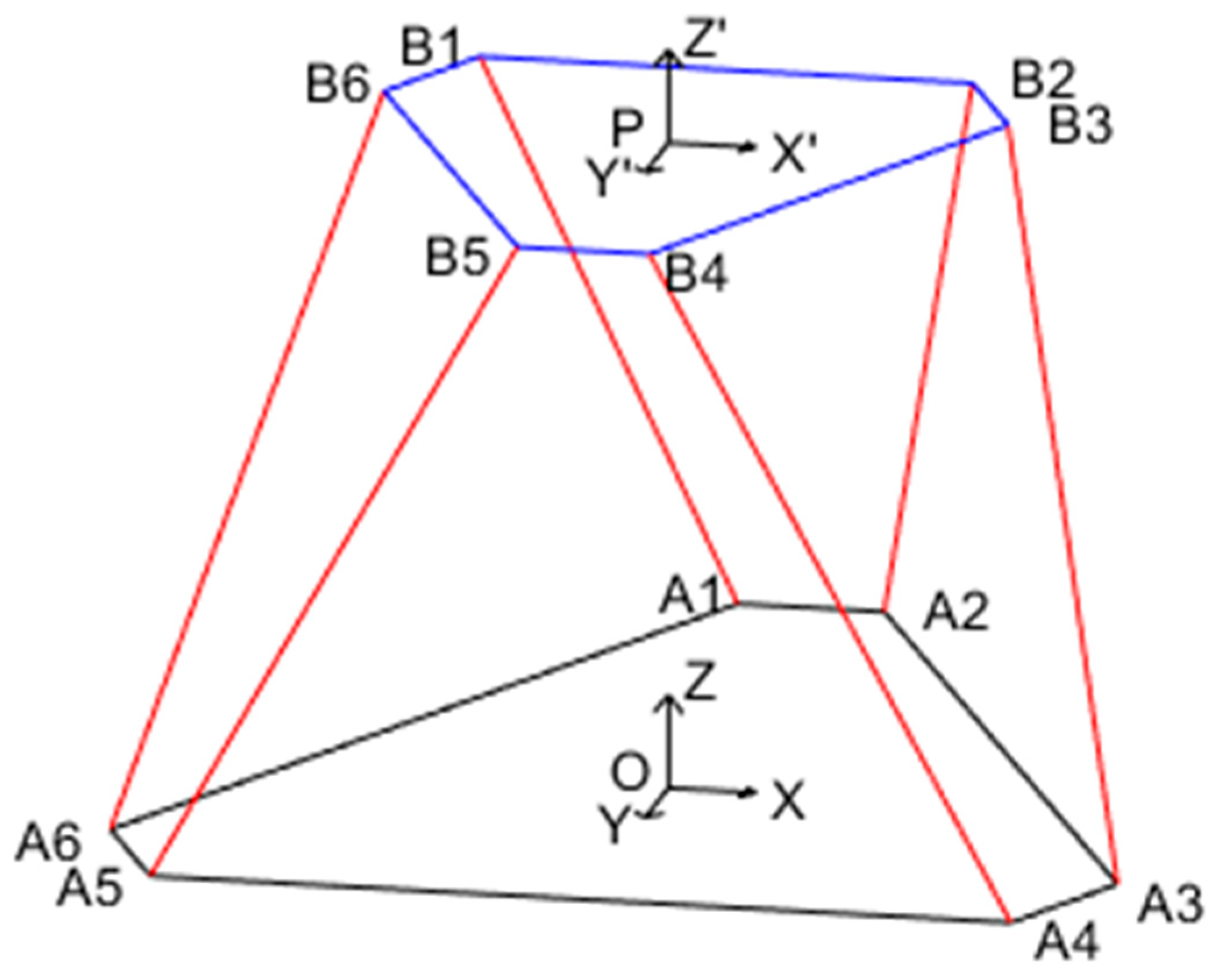
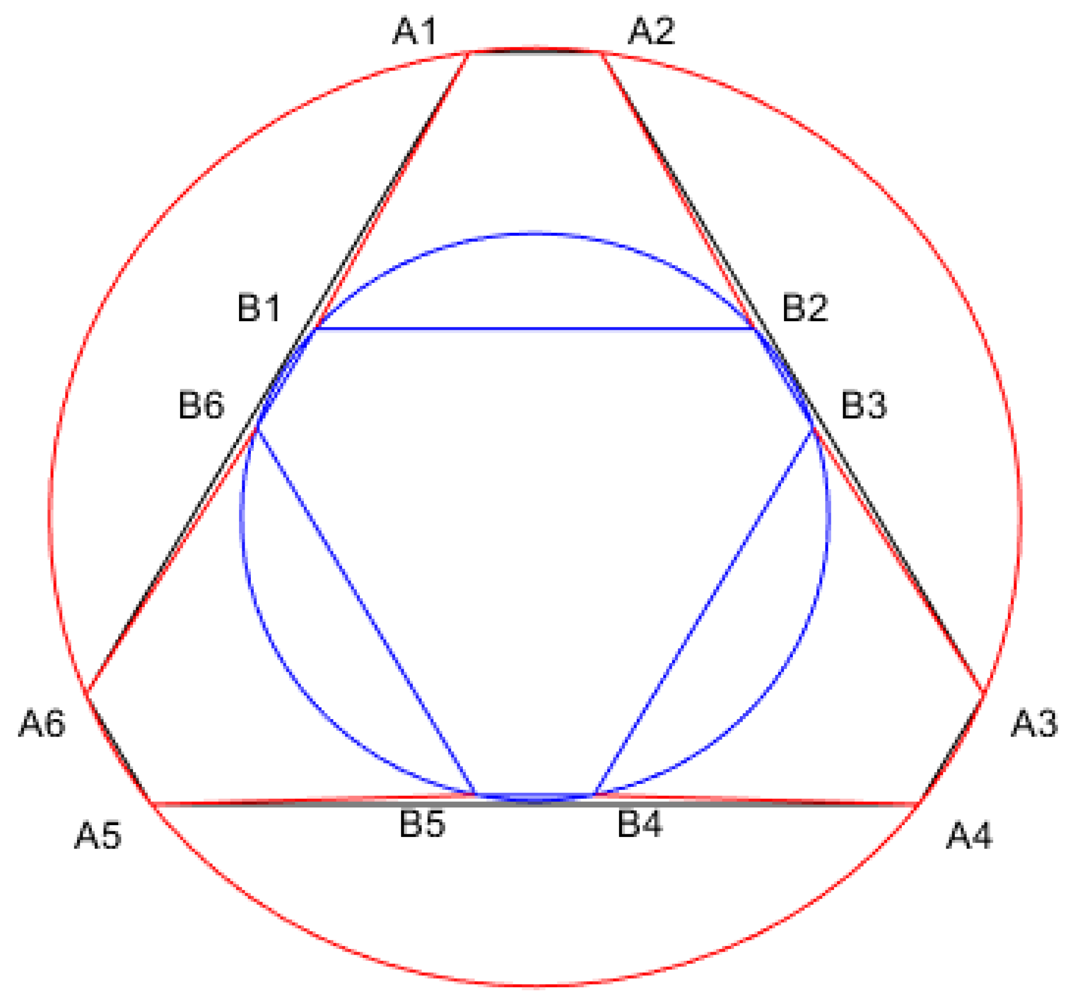
2.1. Kinematic Modeling
2.2. Dataset
2.3. Parallel Platform Jacobian Matrix
2.4. Forward Solution Algorithm of Newton–Raphson Kinematics
2.5. Kinematics forward Solution Algorithm Based on Multivariate Polynomial Regression
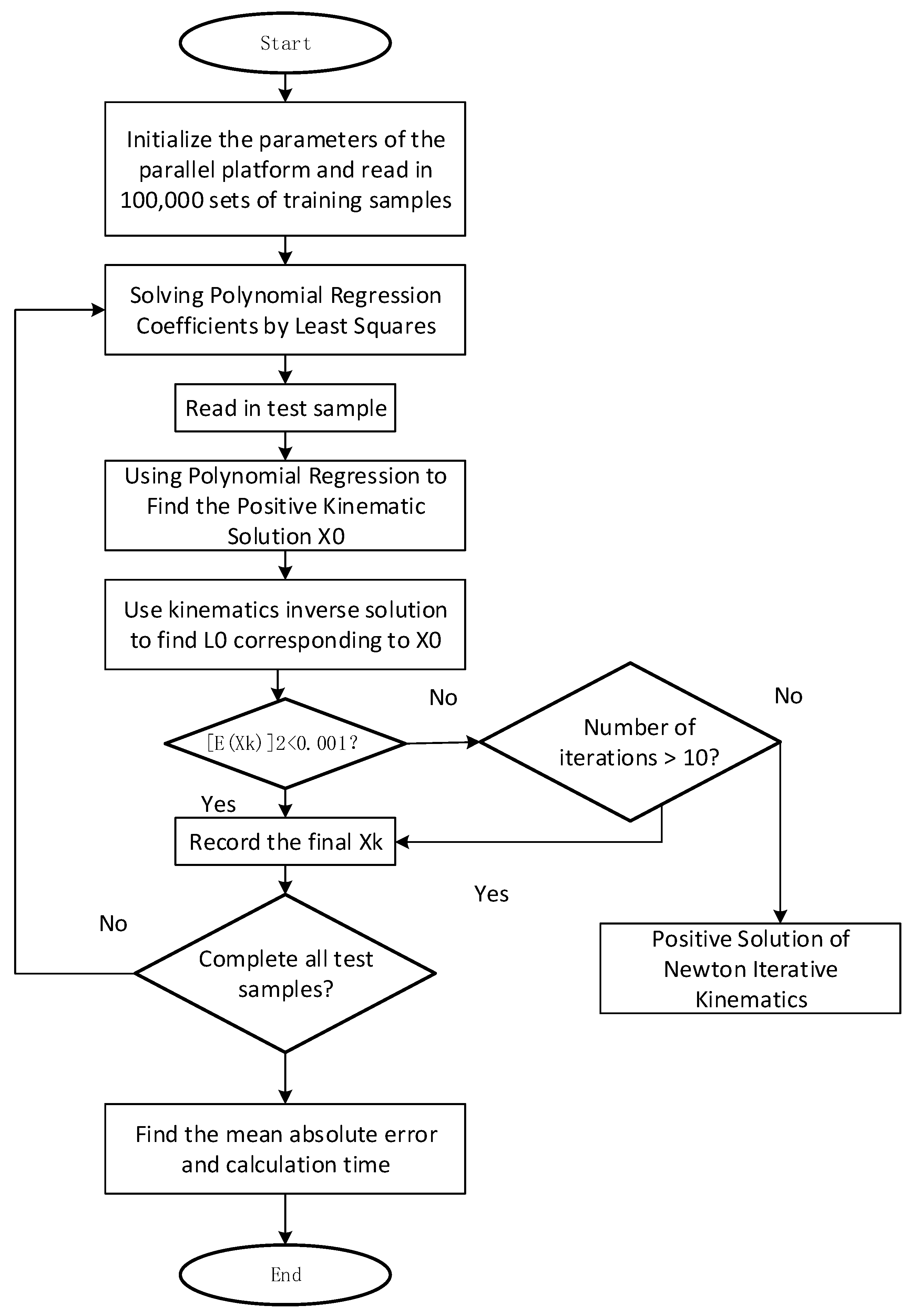
2.6. MPR-NR Algorithm Design
3. Results
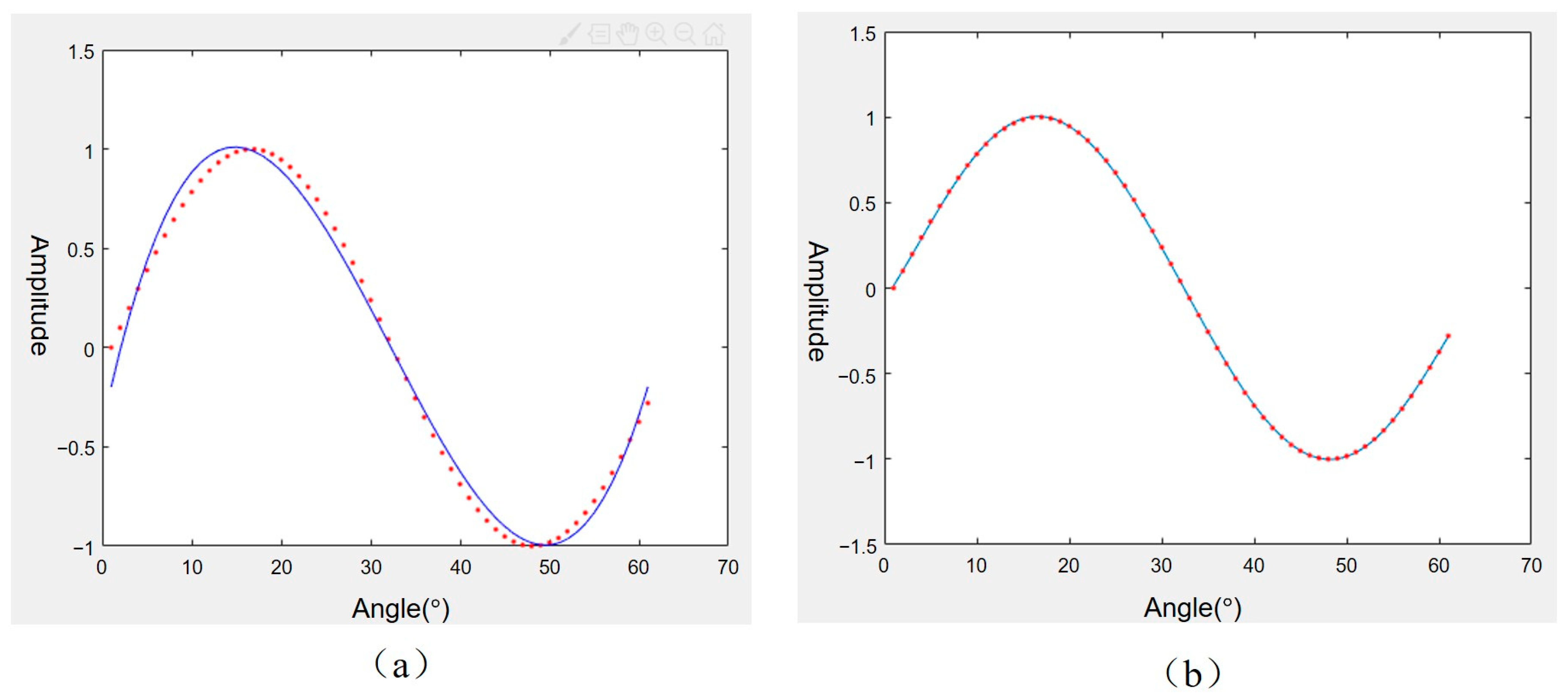
3.1. Single Algorithm Simulation
3.2. MPR-NR Algorithm Simulation
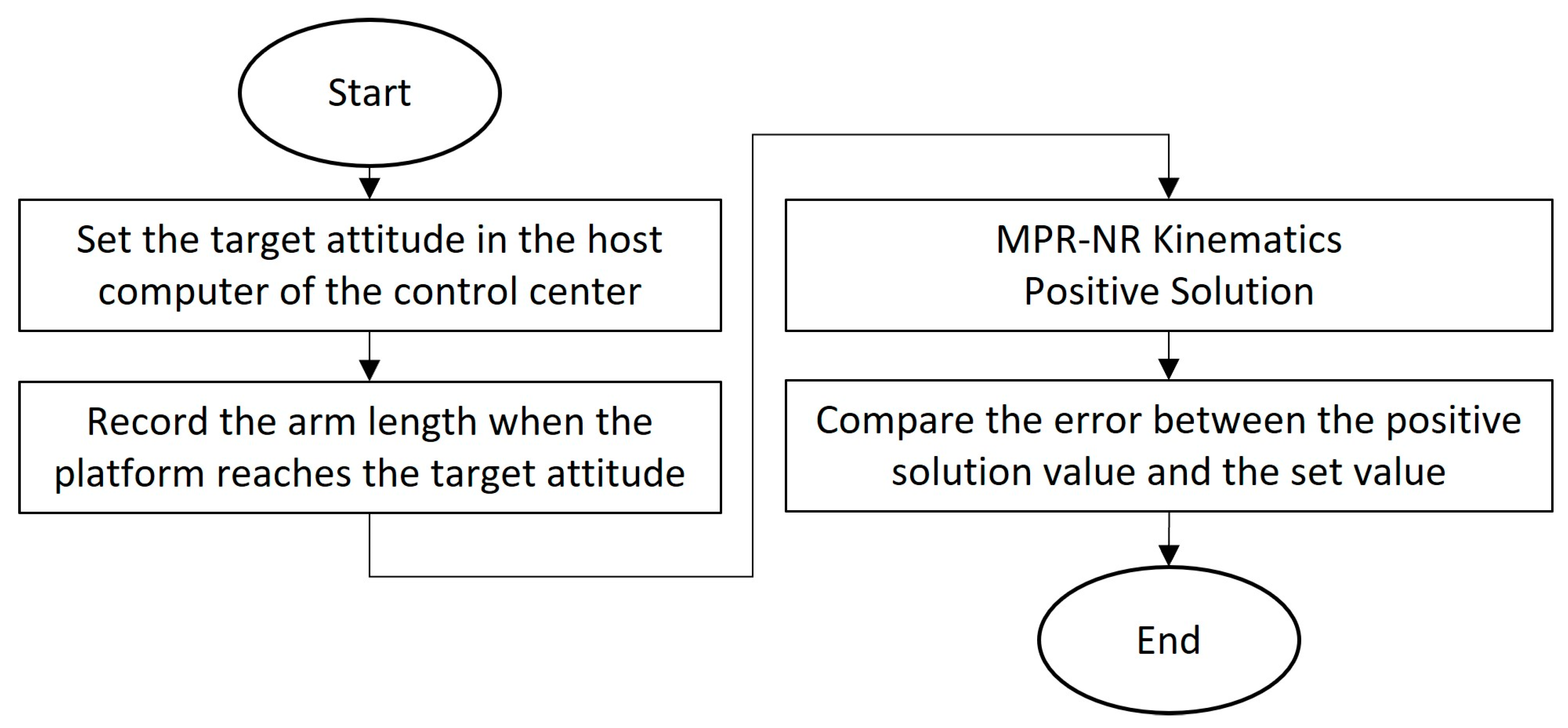
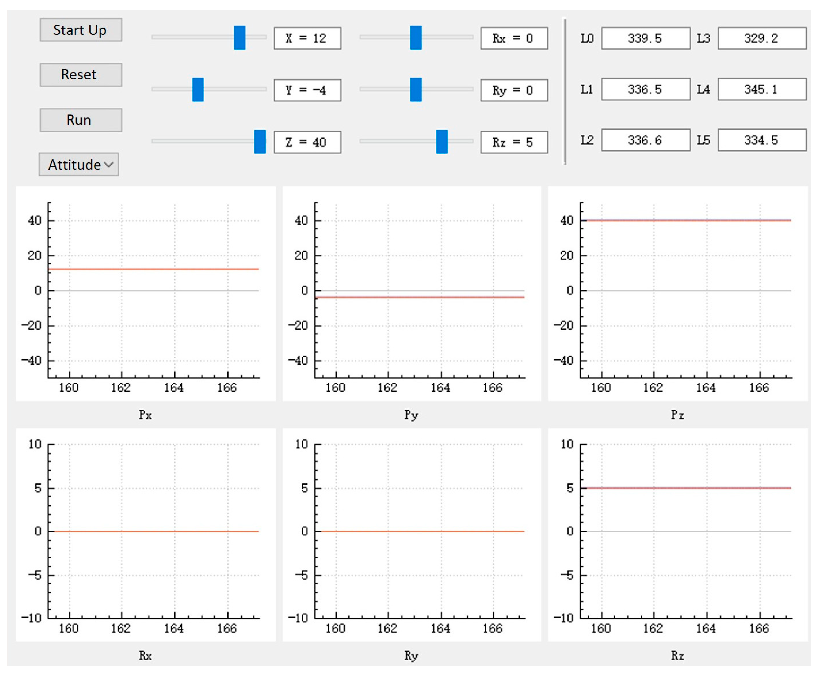
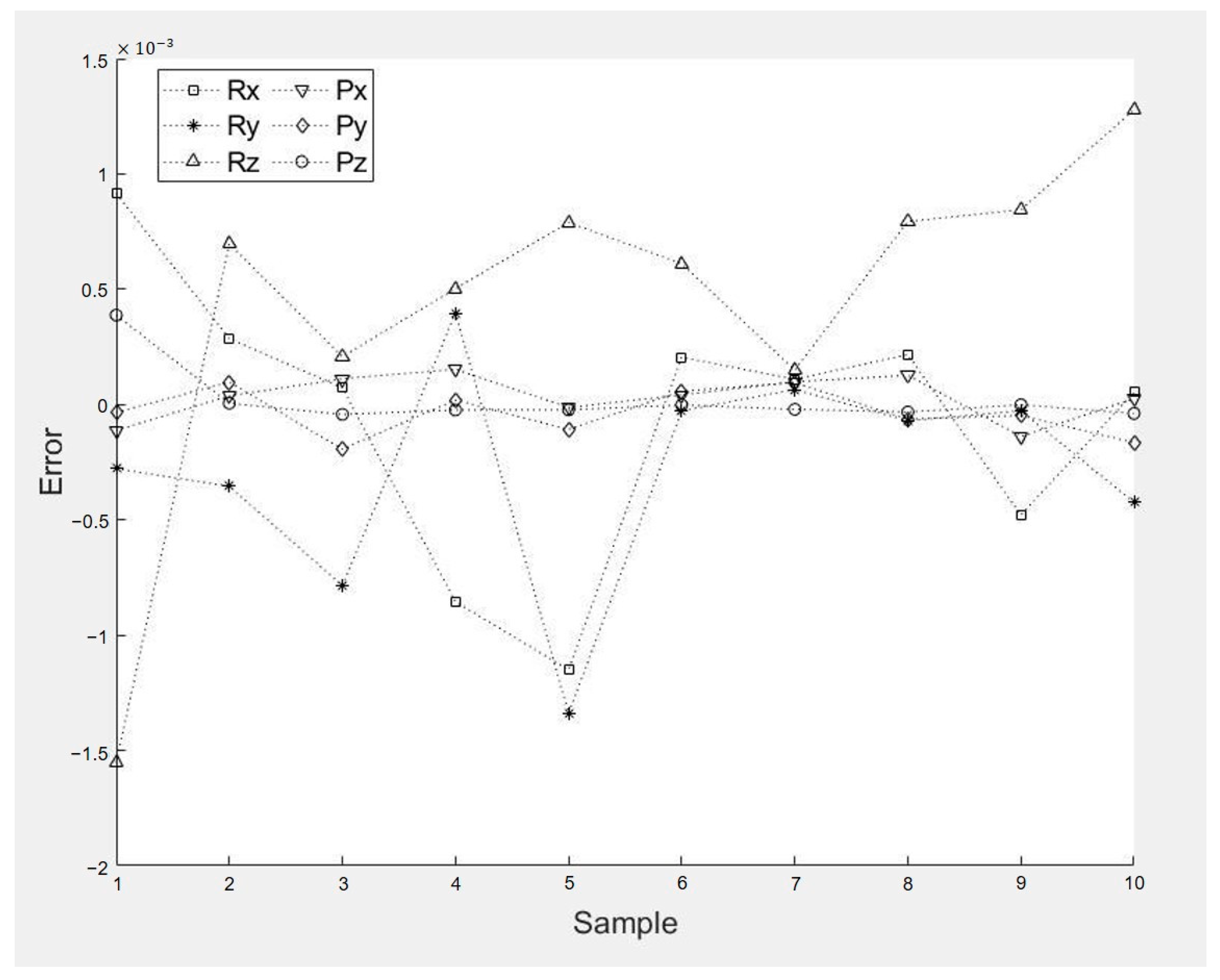
3.3. Physical Test
4. Discussion and Conclusions
Author Contributions
Funding
Institutional Review Board Statement
Informed Consent Statement
Data Availability Statement
Conflicts of Interest
References
- Zahedi, A.; Shafei, A.; Shamsi, M. Kinetics of planar constrained robotic mechanisms with multiple closed loops: An experimental study. Mech. Mach. Theory 2023, 183, 105250. [Google Scholar] [CrossRef]
- Bhaskar, D.; Mruthyunjaya, T.S. A Newton-Euler formulation for the inverse dynamics of the Stewart platform manipulator. Mech. Mach. Theory 1998, 33, 1135–1152. [Google Scholar]
- Leroy, N.; Kokosy, A.M.; Perruquetti, W. Dynamic modeling of a parallel robot, Application to a surgical simulator. In Proceedings of the IEEE International Conference on Robotics and Automation, Taipei, Taiwan, 14–19 September 2003; pp. 4330–4335. [Google Scholar]
- Gallardo, J.; Rico, J.M.; Frisoli, A.; Checcacci, D.; Bergamasco, M. Dynamics of parallel manipulators by means of screw theory. Mech. Mach. Theory 2003, 38, 1113–1131. [Google Scholar] [CrossRef]
- Tsai, L. Solving the Inverse Dynamics of a Stewart-Gough Manipulator by the Principle of Virtual Work. J. Mech. Des. 2000, 122, 3–9. [Google Scholar] [CrossRef]
- Nouri Rahmat Abadi, B.; Mahzoon, M.; Farid, M. Singularity-Free Trajectory Planning of a 3-RP RR Planar Kinematically Redundant Parallel Mechanism for Minimum Actuating Effort. Iran. J. Sci. Technol. Trans. Mech. Eng. 2019, 43, 739–751. [Google Scholar] [CrossRef]
- Sumnu, A.; Güzelbey, I.H.; Cakır, M.V. Simulation and PID control of a Stewart platform with linear motor. J. Mech. Sci. Technol. 2017, 31, 345–356. [Google Scholar] [CrossRef]
- Kazezkhan, G.; Xiang, B.; Wang, N.; Yusup, A. Dynamic modeling of the Stewart platform for the NanShan Radio Telescope. Adv. Mech. Eng. 2020, 12, 1687814020940072. [Google Scholar] [CrossRef]
- Tang, J.; Cao, D.; Yu, T. Decentralized vibration control of a voice coil motor-based Stewart parallel mechanism: Simulation and experiments. J. Mech. Eng. Sci. 2019, 233, 132–145. [Google Scholar] [CrossRef]
- Behi, F. Kinematic analysis for a six-degree-of-freedom 3-PRPS parallel mechanism. IEEE J. Robot. Autom. 1988, 4, 561–565. [Google Scholar] [CrossRef]
- Zanganeh, K.E.; Sinatra, R.; Angeles, J. Kinematics and dynamics of a six-degree-of-freedom parallel manipulator with revolute legs. Robotica 1997, 15, 385–394. [Google Scholar] [CrossRef]
- Mueller, A. An overview of formulae for the higher-order kinematics of lower-pair chains with applications in robotics and mechanism theory. Mech. Mach. Theory 2019, 142, 103594. [Google Scholar] [CrossRef]
- Guo, D.; Xie, Z.; Sun, X.; Zhang, S. Dynamic Modeling and Model-Based Control with Neural Network-Based Compensation of a Five Degrees-of-Freedom Parallel Mechanism. Machines 2023, 11, 195. [Google Scholar] [CrossRef]
- Nouri Rahmat Abadi, B.; Carretero, J.A. Modeling and Real-Time Motion Planning of a Class of Kinematically Redundant Parallel Mechanisms with Reconfigurable Platform. J. Mech. Robot. 2023, 15, 021004. [Google Scholar] [CrossRef]
- Abadi, B.N.R.; Farid, M.; Mahzoon, M. Redundancy resolution and control of a novel spatial parallel mechanism with kinematic redundancy. Mech. Mach. Theory 2019, 133, 112–126. [Google Scholar] [CrossRef]
- Abadi, B.N.R.; Taghvaei, S.; Vatankhah, R. Optimal motion planning of a planar parallel manipulator with kinematically redundant degrees of freedom. Trans. Can. Soc. Mech. Eng. 2016, 40, 383–397. [Google Scholar] [CrossRef] [Green Version]
- Shimizu, M.; Kakuya, H.; Yoon, W.-K.; Kitagaki, K.; Kosuge, K. Analytical inverse kinematic computation for 7-DOF redundant manipulators with joint limits and its application to redundancy resolution. IEEE Trans. Robot. 2008, 24, 1131–1142. [Google Scholar] [CrossRef]
- Nakamura, Y.; Hanafusa, H. Inverse kinematic solutions with singularity robustness for robot manipulator control. J. Dyn. Syst. Meas. Control 1986, 108, 163–171. [Google Scholar] [CrossRef]
- Sciavicco, L.; Siciliano, B. A solution algorithm to the inverse kinematic problem for redundant manipulators. IEEE J. Robot. Autom. 1988, 4, 403–410. [Google Scholar] [CrossRef]
- Dasgupta, B.; Mruthyunjaya, T. The Stewart platform manipulator: A review. Mech. Mach. Theory 2000, 35, 15–40. [Google Scholar] [CrossRef]
- Nguyen, C.C.; Antrazi, S.C.; Zhou, Z.-L.; Campbell, C.E., Jr. Analysis and implementation of a 6 DOF Stewart Platform-based robotic wrist. Comput. Electr. Eng. 1991, 17, 191–203. [Google Scholar] [CrossRef]
- Chen, D.; Zhang, Y.; Li, S. Tracking control of robot manipulators with unknown models: A jacobian-matrix-adaption method. IEEE Trans. Ind. Inform. 2017, 14, 3044–3053. [Google Scholar] [CrossRef]
- Umetani, Y.; Yoshida, K. Resolved motion rate control of space manipulators with generalized Jacobian matrix. IEEE Trans. Robot. Autom. 1989, 5, 303–314. [Google Scholar] [CrossRef]
- Akram, S.; Ann, Q.U. Newtonaphsonn method. Int. J. Sci. Eng. Res. 2015, 6, 1748–1752. [Google Scholar]
- Yang, C.F.; Zheng, S.T.; Jin, J.; Zhu, S.B.; Han, J.W. Forward kinematics analysis of parallel manipulator using modified global Newton-Raphson method. J. Cent. South Univ. Technol. 2010, 17, 1264–1270. [Google Scholar] [CrossRef]
- De Castro, Y.; Gamboa, F.; Henrion, D.; Hess, R.; Lasserre, J.-B. Approximate optimal designs for multivariate polynomial regression. Ann. Stat. 2019, 47, 127–155. [Google Scholar] [CrossRef] [Green Version]
- Pinkus, A. Weierstrass and approximation theory. J. Approx. Theory 2000, 107, 1–66. [Google Scholar] [CrossRef] [Green Version]
- Sinha, P. Multivariate polynomial regression in data mining: Methodology, problems and solutions. Int. J. Sci. Eng. Res. 2013, 4, 962–965. [Google Scholar]


| Coordinate Points | (mm) | (mm) | (mm) |
|---|---|---|---|
| A1 | −25 | 184 | 52.5 |
| A2 | 25 | 184 | 52.5 |
| A3 | 171.85 | −70.35 | 52.5 |
| A4 | 146.85 | −113.65 | 52.5 |
| A5 | −146.85 | −113.65 | 52.5 |
| A6 | −171.85 | −70.35 | 52.5 |
| B1 | −84.01 | 74.49 | 325.4 |
| B2 | 84.01 | 74.49 | 325.4 |
| B3 | 106.51 | 35.51 | 325.4 |
| B4 | 22.50 | −110 | 325.4 |
| B5 | −22.50 | −110 | 325.4 |
| B6 | −106.51 | 35.51 | 325.4 |
| Algorithm | Dataset | Kinematics Positive Solution Mean Absolute Error | Time |
|---|---|---|---|
| Newton iteration | Test Set 1 | 1.144 | |
| Test Set 2 | 1.815 | ||
| MPR2 | Test Set 1 | 0.169 | |
| Test Set 2 | 0.164 | ||
| MPR3 | Test Set 1 | 0.287 | |
| Test Set 2 | 0.272 |
| Algorithm | Dataset | Kinematics Positive Solution Mean Absolute Error | Time | Iterations |
|---|---|---|---|---|
| Newton iteration | Test Set 1 | 1.144 | 26,710 | |
| Test Set 2 | 1.815 | 41,664 | ||
| MPR2-NR | Test Set 1 | 0.296 | 0 | |
| Test Set 2 | 1.284 | 26,019 | ||
| MPR3-NR | Test Set 1 | 0.407 | 0 | |
| Test Set 2 | 1.162 | 16,998 |
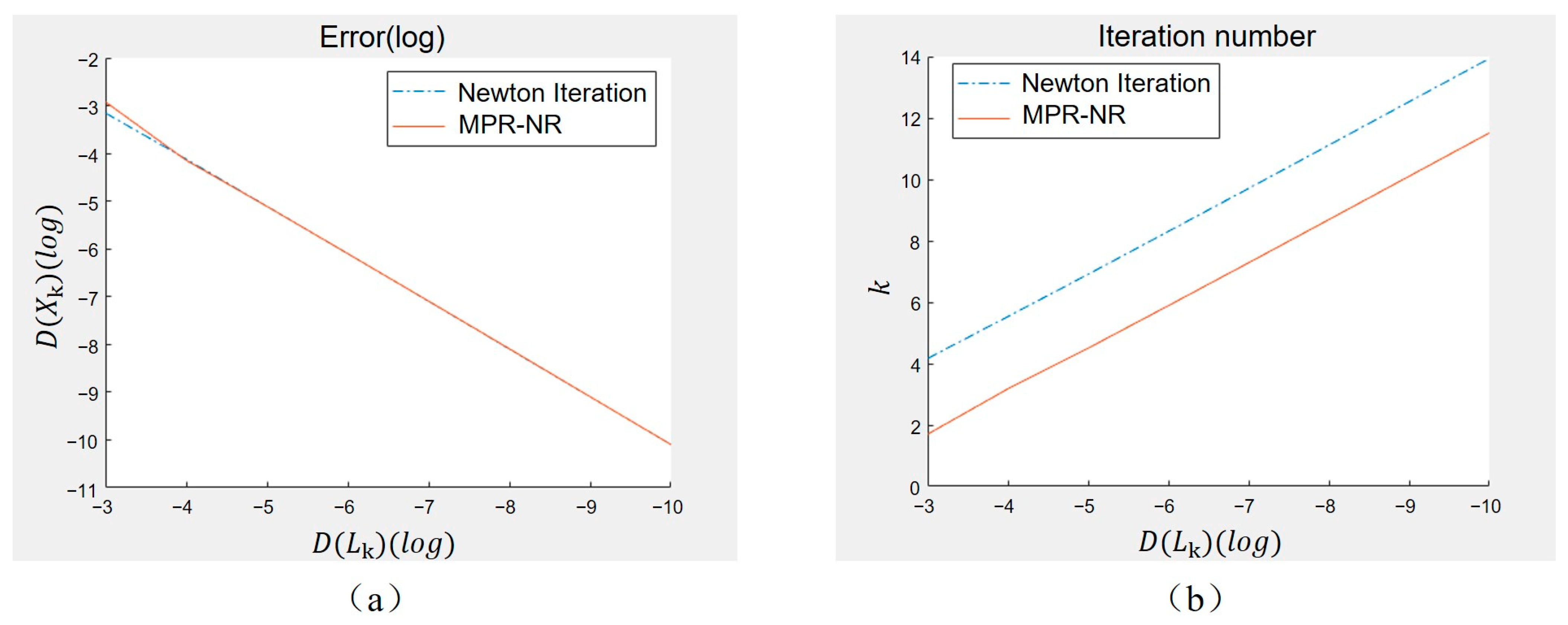
| Newton Algorithm | Average Number of Iterations | MPR-NR | Average Number of Iterations | |
|---|---|---|---|---|
| 1 × 10⁻³ | 7.00 × 10⁻⁴ | 4.16 | 1.20 × 10⁻³ | 1.70 |
| 1 × 10⁻⁴ | 7.59 × 10⁻⁵ | 5.53 | 7.19 × 10⁻⁵ | 3.18 |
| 1 × 10⁻⁵ | 7.81 × 10⁻⁶ | 6.91 | 7.74 × 10⁻⁶ | 4.50 |
| 1 × 10⁻⁶ | 7.96 × 10⁻⁷ | 8.31 | 7.93 × 10⁻⁷ | 5.89 |
| 1 × 10⁻⁷ | 8.01 × 10⁻⁸ | 9.71 | 8.07 × 10⁻⁸ | 7.28 |
| 1 × 10⁻⁸ | 7.99 × 10⁻⁹ | 11.12 | 8.09 × 10⁻⁹ | 8.69 |
| 1 × 10⁻⁹ | 7.99 × 10⁻¹⁰ | 12.53 | 8.01 × 10⁻¹⁰ | 10.10 |
| 1 × 10⁻¹⁰ | 8.03 × 10⁻¹¹ | 13.94 | 7.98 × 10⁻¹¹ | 11.51 |
| Attitude Parameter | Reference Value | Calculation Value |
|---|---|---|
| 0 | −1.68 × 10⁻⁴ | |
| 0 | 5.83 × 10⁻⁵ | |
| 0.0870 | 0.0896 | |
| 0.0120 | 0.0120 | |
| −0.0040 | −0.0040 | |
| 0.0400 | 0.0398 |
Disclaimer/Publisher’s Note: The statements, opinions and data contained in all publications are solely those of the individual author(s) and contributor(s) and not of MDPI and/or the editor(s). MDPI and/or the editor(s) disclaim responsibility for any injury to people or property resulting from any ideas, methods, instructions or products referred to in the content. |
© 2023 by the authors. Licensee MDPI, Basel, Switzerland. This article is an open access article distributed under the terms and conditions of the Creative Commons Attribution (CC BY) license (https://creativecommons.org/licenses/by/4.0/).
Share and Cite
Liu, M.; Gu, Q.; Yang, B.; Yin, Z.; Liu, S.; Yin, L.; Zheng, W. Kinematics Model Optimization Algorithm for Six Degrees of Freedom Parallel Platform. Appl. Sci. 2023, 13, 3082. https://doi.org/10.3390/app13053082
Liu M, Gu Q, Yang B, Yin Z, Liu S, Yin L, Zheng W. Kinematics Model Optimization Algorithm for Six Degrees of Freedom Parallel Platform. Applied Sciences. 2023; 13(5):3082. https://doi.org/10.3390/app13053082
Chicago/Turabian StyleLiu, Mingzhe, Qiuxiang Gu, Bo Yang, Zhengtong Yin, Shan Liu, Lirong Yin, and Wenfeng Zheng. 2023. "Kinematics Model Optimization Algorithm for Six Degrees of Freedom Parallel Platform" Applied Sciences 13, no. 5: 3082. https://doi.org/10.3390/app13053082