Greenhouse Temperature Prediction Based on Time-Series Features and LightGBM

Abstract

A method of establishing a prediction model of the greenhouse temperature based on time-series analysis and the boosting tree model is proposed, aiming at the problem that the temperature of a greenhouse cannot be accurately predicted owing to nonlinear changes in the temperature of the closed ecosystem of a greenhouse featuring modern agricultural technology and various influencing factors. This model comprehensively considers environmental parameters, including humidity inside and outside the greenhouse, air pressure inside and outside the greenhouse, and temperature outside the greenhouse, as well as time-series changes, to make a more accurate prediction of the temperature in the greenhouse. Experiments show that the R² determination coefficients of different prediction models are improved and the mean square error and mean absolute error are reduced after adding time-series features. Among the models tested, LightGBM performs best, with the mean square error of the prediction results of the model decreasing by 18.61% after adding time-series features. Comparing with the support vector machine, radial basis function neural network, back-propagation neural network, and multiple linear regression model after adding time-series features, the mean square error is 11.70% to 29.12% lower. Furthermore, the fitting degree of LightGBM is the best among the models. The prediction results of LightGBM therefore have important application value in greenhouse temperature control.

1. Introduction

China has gradually transformed from traditional agriculture to modern agriculture and is gradually moving towards intelligent agriculture with the development of computer technology. A greenhouse is a typical scene of the application of modern agricultural technology in that its internal environment is operable. A greenhouse can form a small, closed ecosystem suitable for plant growth and improve the yield and quality of agricultural products, and it is thus used widely in agricultural production. Among the environmental factors of a greenhouse, crops are most sensitive to temperature. Temperature affects the enzyme activity of plant cells and thus the growth rate, yield, and quality of crops, i.e., temperature strongly affects the growth and development of crops. In ensuring the yield and quality of agricultural products, we should ensure the normal growth of crops by accurately controlling the greenhouse temperature.

2. Related Work

Recent theoretical research on the temperature of a greenhouse environment mainly includes the investigation of the prediction model of energy and the material balance equation, but the thinking of factors affecting the indoor environment is too singular, and time-series features and environmental factors of a greenhouse have not been comprehensively considered [1,2]. Cui Lizhen et al. [3] adopted the improved support vector machine (SVM) and grid search algorithm. It is possible to dynamically optimize the kernel parameters and penalty factors of the SVM, but the grid search efficiency is too low, and more computing resources are needed to handle increasing data volumes. Peng Xiuyuan et al. [4,5] used the least-squares method to predict the temperature curve but only predicted the future temperature according to the historical change in temperature and did not consider other environmental factors, such as the air pressure and humidity. Yu Chaogang et al. [6,7] established a model for predicting the greenhouse indoor temperature adopting a radial basis function (RBF) neural network, which has a high training speed and does not fall into local optima, but they did not consider the nonlinear effects of environmental factors on the greenhouse temperature. Zhang Kun’ao et al. [8,9] adopted particle swarm optimization (PSO) to optimize the prediction of the greenhouse temperature. A PSO algorithm can optimize the RBF neural network structure and network weights can improve the training performance. However, with increases in the number of sample data, the number of model iterations, and particle size, the prediction results of the model are prone to be trapped in local optima. Sam Nguyen Xuan et al. [10,11] tested and predicted the influencing factors of the indoor temperature adopting a dynamic model and multiple linear regression. They comprehensively considered a variety of environmental factors, such as the indoor temperature and humidity and outdoor temperature. However, some factors of multiple linear regression are not measurable, and it must be assumed that the environment is a small ecosystem in which the conservation of energy holds, but this situation does not occur in reality. Fen He et al. established a temperature prediction model for the greenhouse ecosystem based on the back-propagation (BP) neural network [12,13]. The model has the characteristics of a simple structure, low calculation cost, and strong adaptability. However, there are many minima in the BP neural network, such that it is easy to fall into local minima. A large number of training times leads to a low learning efficiency and slow convergence. The selection of the hidden layer lacks theoretical guidance, and there is a tendency to forget the old samples when training and learning new samples. Georgia Papacharalampous et al. carried out the time-series analysis of a hydrological climate and extracted many time-series features, such as trend features and extreme features, which affected the accuracy of the hydrological climate prediction [14]. In recent years, multivariate time series was proposed. Ziyu Jia et al. [15] proposed a theory of state space reconstruction of multivariate time series based on the non-uniform embedding method of information theory, and in [16] they present a new non-uniform embedding method framed in information theory to detect causality for multivariate time series, named LM-PMIME. The key to solving the problem of multivariate time-series prediction lies in the description of the relationship between the variables. Only by accurately and clearly expressing the mutual influence of each variable can we achieve good prediction results. In other words, the prediction effect of multivariate time series with an unclear relationship is not satisfactory.

In view of the above problems, this paper uses the light gradient boosting machine (LightGBM) model as the basic prediction model. LightGBM not only applies a series of environmental factors, such as humidity, air pressure, and outdoor temperature, to the prediction of the greenhouse temperature, but also comprehensively considers temporal and nonlinear changes in indoor and outdoor temperature. Adopting environmental factors and a time-series feature extraction method proposed in the literature [14], a greenhouse temperature prediction model is established to make a more accurate prediction of the greenhouse temperature and thus improve the quality and yield of crops and avoid unnecessary economic losses resulting from inaccurate prediction.

3. Proposed Methodology

The proposed method is based on LightGBM, which is a framework for implementing the gradient boosting decision tree (GBDT) algorithm developed by Microsoft. The GBDT algorithm is an iterative-based decision tree algorithm. It uses the classification and regression tree model as the weak learner. The new learner is established in the direction that the gradient of the loss function of the previous learner falls, and the new learner is then iteratively generated to train the model [17]. In the iterative process, the next round of prediction is based on the residual between the predicted value and the real value of the previous round, and all the predicted results are added as the conclusion. The GBDT algorithm can therefore be expressed as the optimization process of decision tree learning with an additive model and forward step algorithm [18]:

$$F_M\left(X\right)={\sum }_{m=1}^M{f}_m\left(X\right),$$

(1)

where $f_m\left(X\right)$ represents the decision tree. M is the number of trees and the number of iterations. The boosting tree is initialized as:

$$F_0\left(X\right)=0.$$

According to the forward step-by-step algorithm, the model of the m-th step can be expressed as:

$$F_m\left(X\right)=F_{m-1}\left(X\right)+f_m\left(X\right),$$

(2)

where $F_{m-1}\left(X\right)$ is the current model and $f_m\left(X\right)$ is the current decision tree. Taking the squared loss as the loss function and supposing that there is a sequence $X$:$x_1,x_2,x_3,\dots ,x_n$ and corresponding true values $Y$: $y_1,y_2,\cdots ,y_n$, the loss function is defined as:

$$L(Y,F_m\left(X\right))=\frac{1}{n}{\sum }_{i=1}^n\left({\left(y_i-F_m\left(x_i\right)\right)}^2\right).$$

(3)

The first derivative of the loss function is:

$$L^{\prime }(Y,F_m\left(X\right))=-\frac{2}{n}{\sum }_{i=1}^n\left(y_i-F_m\left(x_i\right)\right).$$

(4)

The second derivative of the loss function is:

$$L^{″}\left(Y,F_m(X\right))=2.$$

(5)

Furthermore, according to Formula (4), we obtained the first derivative of the loss function as:

$$L^{\prime }\left(Y,F_m(X\right))=L^{\prime }\left(Y,F_{m-1}\left(X\right)+f_m\left(X\right)\right)$$

(6)

while according to the first-order expansion of the Taylor formula,

$$f\left(x+x_0\right)=f\left(x\right)+f^{\prime }\left(x\right)\times x_0,$$

(7)

We have:

$$L^{\prime }\left(Y,F_m(X\right))=L^{\prime }\left(Y,F_{m-1}\left(X\right)\right)+L^{″}\left(Y,F_{m-1}\left(X\right)\right)\times f_m\left(X\right).$$

(8)

We obtained the best tree when $L^{\prime }\left(Y,F_m(X\right))=0$. It follows that:

$$f_m\left(X\right)=-\frac{L^{\prime }\left(Y,F_{m-1}\left(X\right)\right)}{L^{″}\left(Y,F_{m-1}\left(X\right)\right)}$$

(9)

According to Formulas (6) and (7):

$$f_m\left(X\right)=-\frac{-\frac{2}{n}{\sum }_{i=1}^n\left(y_i-F_{m-1}\left(x_i\right)\right)}{2}=\frac{1}{n}{\sum }_{i=1}^n\left(y_i-F_{m-1}\left(x_i\right)\right),$$

(10)

and it follows from Formula (4) that:

$$F_m\left(X\right)=F_{m-1}\left(X\right)+\frac{1}{n}{\sum }_{i=1}^n\left(y_i-F_{m-1}\left(x_i\right)\right).$$

(11)

Finally, we obtained the strong learner as:

$$F_M\left(X\right)=F_0\left(X\right)+\frac{1}{n}{\sum }_{m=1}^M{\sum }_{i=1}^n\left(y_i-F_{m-1}\left(x_i\right)\right).$$

(12)

In the above formula, $n$ is the total number of samples. The model of the optimal solution was obtained by iteration.

The conventional implementation of the GBDT requires the scanning of all the data instances to estimate the information gain of all the possible split points [19]. The implementation is thus time-consuming when handling big data. LightGBM uses a histogram-based algorithm (Histogram) to traverse each segmentation point, which consumes less memory and reduces the complexity of data separation to speed up the training process. It also uses the gradient-based one-side sampling algorithm to reduce a large amount of data with only small gradients, uses the exclusive features bundling algorithm to bind many mutually exclusive features into one feature, and uses the leaf-wise strategy to grow trees and find the leaf with the largest gain of variance for the split [20]. LightGBM thus has the advantages of faster training, lower memory consumption, better accuracy, and quicker processing of massive data. LightGBM is therefore widely used for ranking, classification, prediction, and many other machine learning tasks [21,22,23,24,25].

4. Experiment

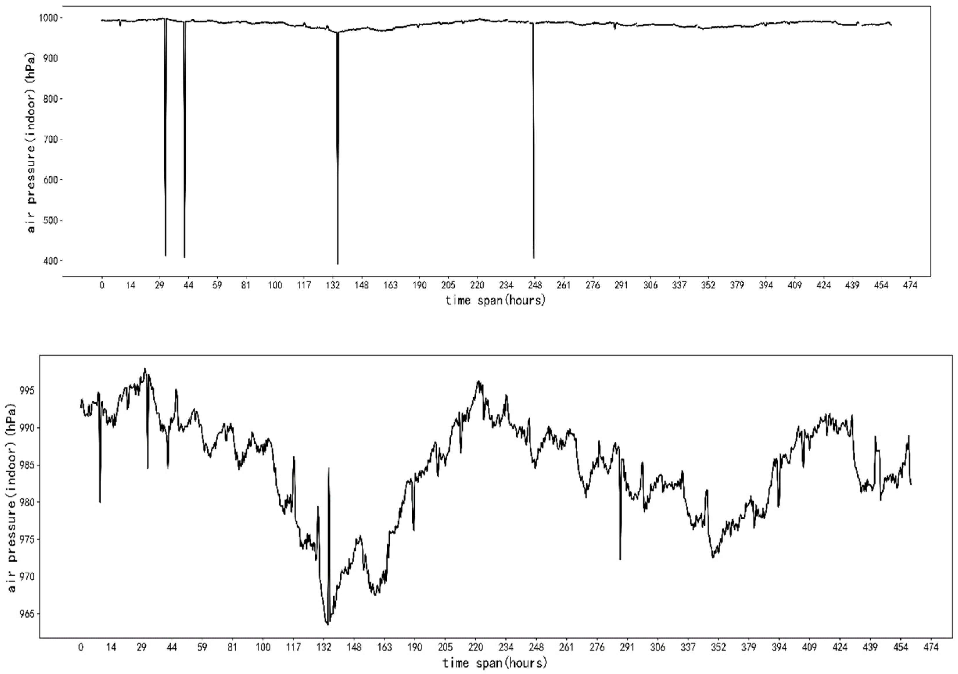
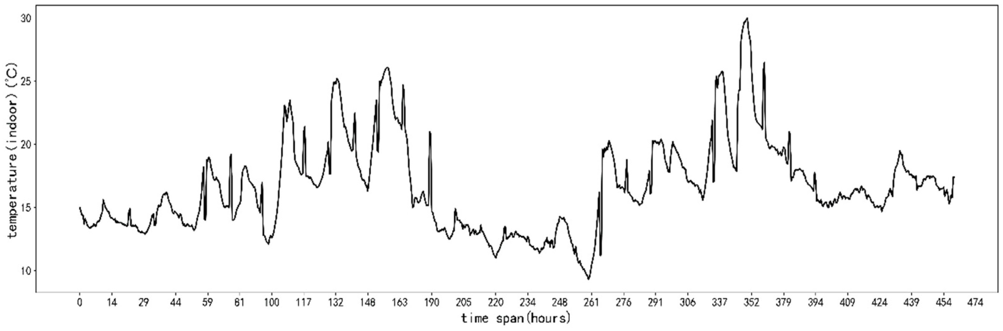
4.1. Data Description

The experimental data were taken from an online competition (2020 iFLYTEK A.I., url: http://challenge.xfyun.cn/topic/info?type=temperature (accessed on 1 July 2020)) held by iFLYTEK. The greenhouse data available on the competition platform were collected by sensors at an experimental station and provided by the China Agricultural University. The collected dataset includes data of the collection time, the temperature, humidity, and air pressure in the greenhouse, and the temperature, humidity, and air pressure outside the greenhouse. The sensors collected data for a total of 30 days from 14 March to 13 April 2019, among which the data of the first 20 days (with each minute of environmental parameters being a group of data) were used as training data and the data of the next 10 days were used as temperature prediction test data. The goal of the experiment was to use the data recorded every minute in the previous 20 days and predict the data every 30 min in the next 10 days. The data descriptions are provided in

Table 1. All original features and descriptions.

Name	Description
Collection time	Data collection time
Temperature (indoor)	Temperature inside greenhouse (Label)
Humidity (indoor)	Humidity inside greenhouse
Air pressure (indoor)	Air pressure inside greenhouse
Temperature (outdoor)	Temperature outside greenhouse
Humidity (outdoor)	Humidity outside greenhouse
Air pressure (outdoor)	Air pressure outside greenhouse

.

There were 25,904 records in the dataset. Except for the collection time having a time format, all the data were of float64 type, and the six fields of the indoor and outdoor temperature, humidity, and air pressure for the greenhouse had missing data to varying degrees. Statistical information of the data, except the collection time, is presented in

Table 2. Statistical analysis of the original features.

	Indoor Temperature (°C)	Indoor Humidity (%)	Indoor Air Pressure (hPa)	Outdoor Temperature (°C)	Outdoor Humidity (%)	Outdoor Air Pressure (hPa)
count	24,807	24,807	24,807	25,241	24,837	24,837
mean	16.63	72.60	981.26	16.61	74.36	983.64
SD	3.69	14.05	43.90	4.32	16.35	22.99
min	9.3	25	392.5	8.9	23	400.2
25%	13.8	64	980	13.4	64	979.9
50%	16.1	76	985.9	16	78	986.1
75%	18.4	84	989.9	18.7	88	990.4
max	30.1	91	1013.7	36.7	96	1082.5

.

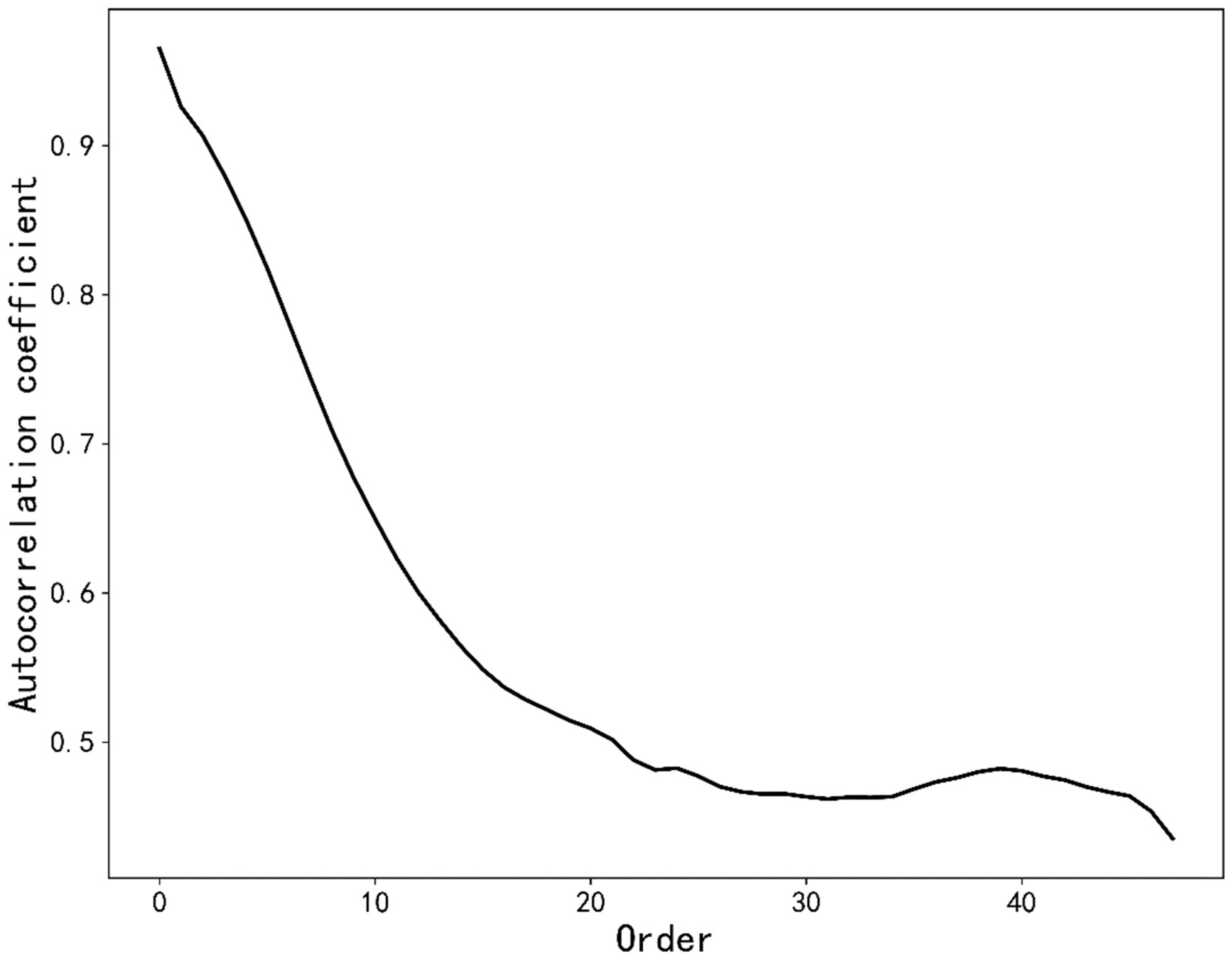
4.2. Data Preprocessing

There may have been equipment abnormalities during the data collection and thus failures in data collection and abnormalities in the collected data. The original data of each category in the dataset are missing to some extent. The forward filling method was used to fill in the missing data. Abnormal data were corrected to a reasonable range. The data distributions before and after correction are shown in Figure 1.

In Figure 1, the value on the horizontal axis is the number of hours after 1:00 on 14 March 2019. The top plot is the indoor air pressure changing with time before data correction. The range of the air pressure is 400–1000 hPa, and there are obvious abnormal data (data deviating from the change trend), which will affect the prediction of the model. We replaced these abnormal data with the average value for the column to reduce their effect and bring the data closer to the trend of change. It is seen that the change in indoor air pressure with time after correction (the lower plot in Figure 1) follows a certain rule. Although a few data deviated from the change trend, they were all within a reasonable range.

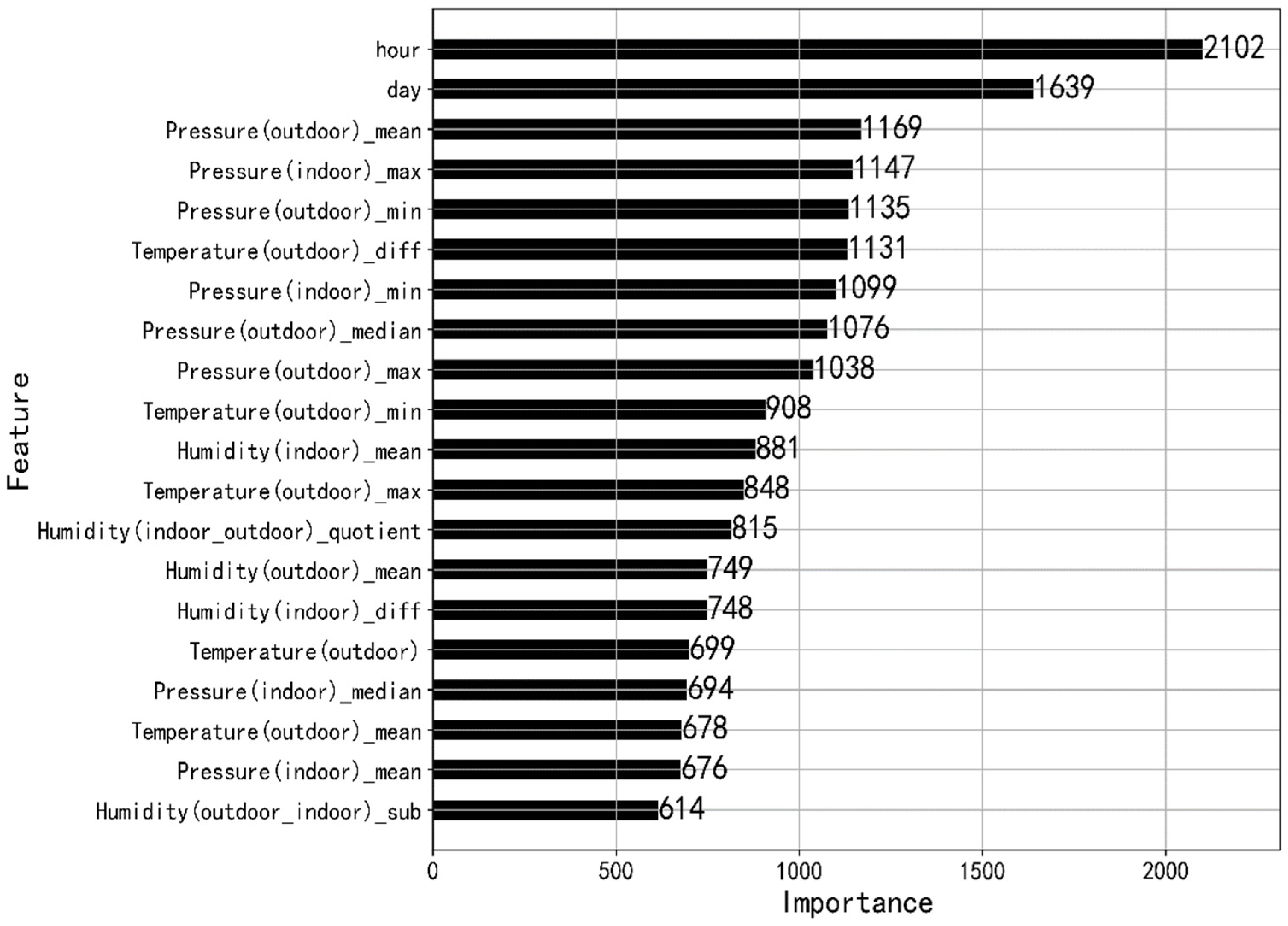
4.3. Feature Engineering

In studying the regularity of time-series data with a change in indoor temperature, the autocorrelation analysis of the indoor temperature was carried out adopting the autocorrelation analysis method [26,27]. The autocorrelation coefficient, which is between 0 and 1, was used as the quantitative indicator of correlation. A larger value indicates higher correlation. Suppose that there is a sequence $X$:$x_1,x_2,x_3,...,x_n$. Let $X_{s,t}$ be the sequence $x_s,x_{s+1},...,{x_{t-1},x}_t$ starting at time s and ending at time t. $u_{s,t}$ is the mean value of the sequence $X_{s,t}$ and ${\sigma }_{s,t}$ is the standard deviation of the sequence $X_{s,t}$. The first-order autocorrelation coefficient is then:

$$R\left(1\right)=\frac{E\left(X_{2,n}-u_{s,n}\right)\ast \left(X_{1,n-1}-u_{1,n-1}\right)}{{\sigma }_{2,n}\ast {\sigma }_{1,n-1}}.$$

(13)

Similarly, the k-order autocorrelation coefficient is:

$$R\left(k\right)=\frac{E\left(X_{k+1,n}-u_{k+1,n}\right)\ast \left(X_{1,n-k}-u_{1,n-k}\right)}{{\sigma }_{k+1,n}\ast {\sigma }_{1,n-k}}.$$

(14)

Adopting Formula (14), the high-order autocorrelation coefficient of the indoor temperature was calculated, and the change in correlation with order is shown in Figure 2.

Figure 2 shows that the correlation gradually decreased with an increase in order, and the coefficient of the time-series correlation of temperature exceeded 0.6 when the order was less than 10 and exceeded 0.8 when the order was particularly low. It is therefore considered that the indoor temperature has a strong time-series correlation within the reasonable order range.

In characterizing the regularity of environmental factors changing with time, the difference in each feature is regarded as a series feature. The collection interval of every two groups of data was 1 min in the training set and 30 min in the test set, and it is thus necessary to set the training set interval to 30 when generating the difference feature (i.e., generating the difference from the data 30 min ago) and to set it to 1 in the test set (i.e., generating a difference from the previous group of data). Based on Figure 2, to ensure that the data have high autocorrelation, only the first-order difference features were used in this paper [28].

Jinan Gu proposed that temperature and time have an exponential relation when environmental factors change [29]. There are static characteristics, such as temperature, air pressure, and humidity, in the dataset that are representative of the moment in time. In generating dynamic characteristics, we let $t$ be the current time. $t-2$, $t-1$, and $t+1$ then denote the two-previous times, previous time, and next time, respectively. We need to use data of the current time (i.e., the data information at time $t$) and previous times to predict the greenhouse temperature at time $t+1$. The time interval of each collection in the test set was 30 min, and the time interval between $t$ and $t+1$ was therefore also 30 min. The indoor temperature change trend in the collected training set is shown in Figure 3. The value on the horizontal axis is the number of hours after 1:00 on 14 March 2019.

We concluded from the change in the temperature autocorrelation with order in Figure 2 that temperature has a high time-series correlation within a certain order range. We then used the original features given in Table 1 to extract the differential features of each influence factor as part of the time-series features [30,31]. As examples, the feature Temperature(outdoor)_diff describes the difference in outdoor temperature from $t-1$ to $t$, the feature Humidity(outdoor)_diff describes the difference in outdoor humidity from $t-1$ to $t$, and the feature Pressure(indoor)_diff describes the difference in indoor air pressure from $t-1$ to $t$.

The difference features only represent the change regularity of environmental factors at the last time or earlier and do not consider the general regularity of environmental factors in the present time range. To reflect the general trend of features, we generated statistical features according to all the data information in a time interval. As an example, if a statistical feature within a time interval is generated, a window size of 30 is needed in the training set, and the mean value, minimum value, maximum value, median, and other attributes of each feature are calculated using the sliding window algorithm [32,33]. As examples, Temperature(outdoor)_min is the minimum value of the outdoor temperature in the sliding window, Humidity(indoor)_mean is the minimum value of the indoor humidity in the sliding window, Pressure(outdoor)_max is the maximum value of the outdoor air pressure in the sliding window, and Pressure(outdoor)_median is the median of the outdoor air pressure in the sliding window.

Statistical features reflect the general trend of environmental factors based on difference features but do not combine relationships between various environmental factors. The relationship between a single environmental factor and indoor temperature may be linear, whereas combined environmental factors and the indoor temperature may have a relationship that is not simply linear. Combined features help us to express the nonlinear relationship between features and labels. Therefore, the combination information of environmental factors was introduced as cross-features (combination features), which can be information obtained by multiplication or taking the Cartesian product of environmental factors. As examples, the feature Humidity(indoor_outdoor)_quotient is the quotient of the outdoor humidity and indoor humidity, the feature Temp(outdoor)_Hum(outdoor)_quotient is the quotient of the outdoor temperature and outdoor humidity, and the feature Pre(outdoor)_Hum(indoor)_quotient is the quotient of indoor humidity and outdoor air pressure.

All the difference and statistical features mentioned above are time-series features. The difference features can be described as the gap between the current time and the previous or earlier time, which allows the model to learn the change trend of environmental factors. Statistical characteristics (e.g., the mean, minimum, maximum, and median) describe the general trend of environmental factors in the time interval. These features are conducive to reducing the effect of outliers in the training process. The difference features, statistical features, and cross-features were input into the LightGBM model for preliminary feature selection. The ranking of the feature importance after selection from high to low is shown in Figure 4 (where only the top 20 features are displayed).

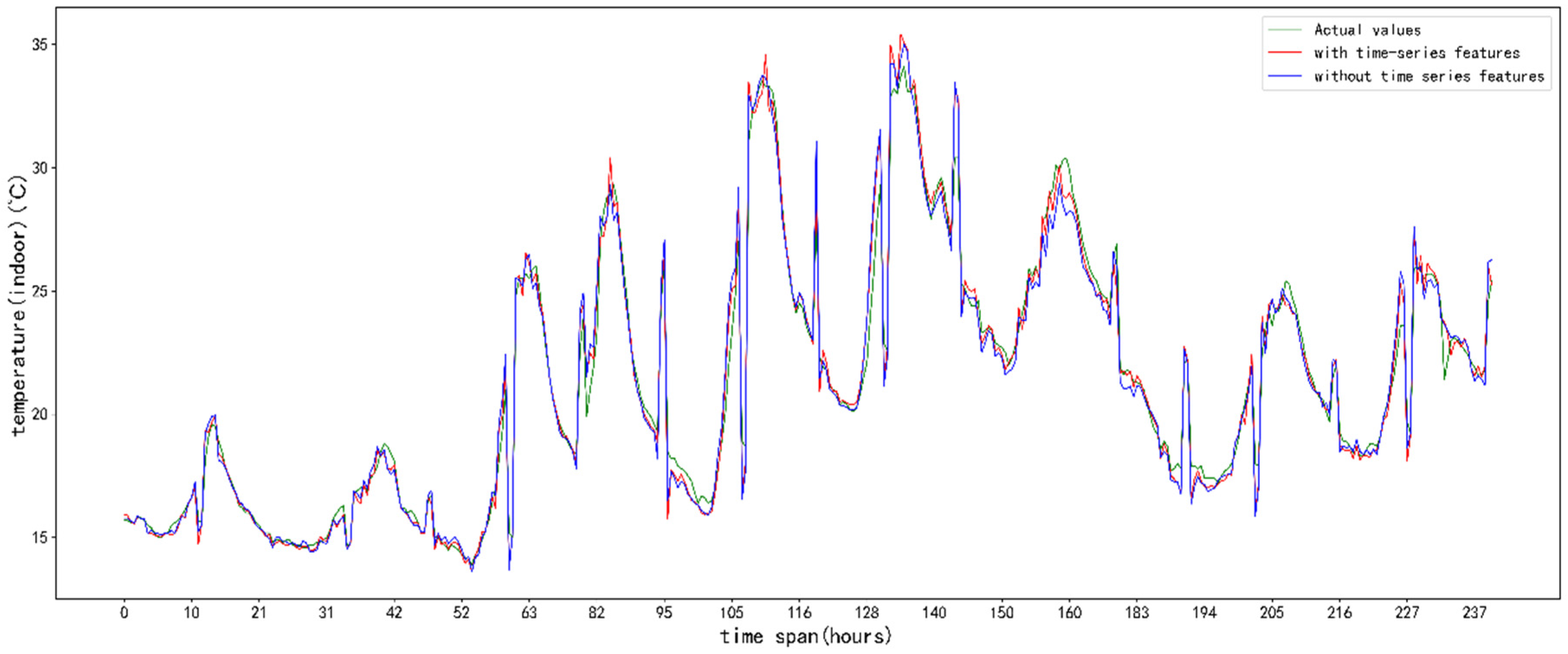
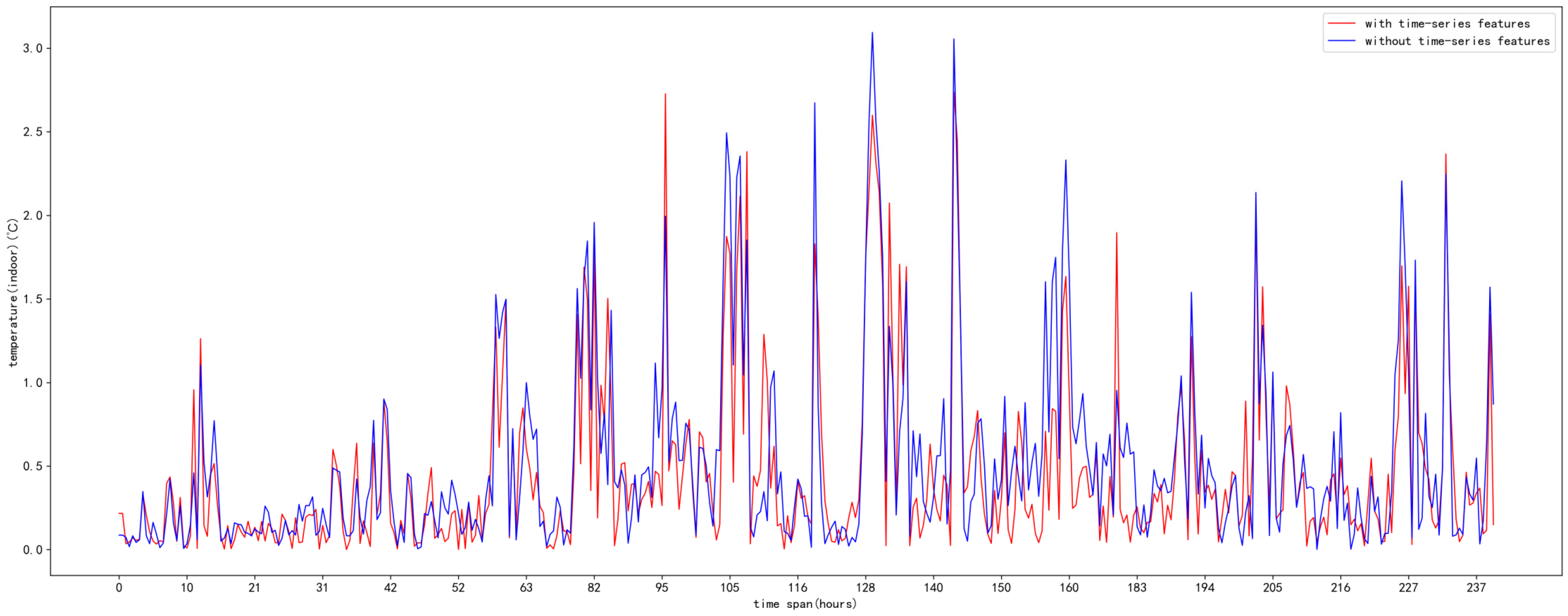
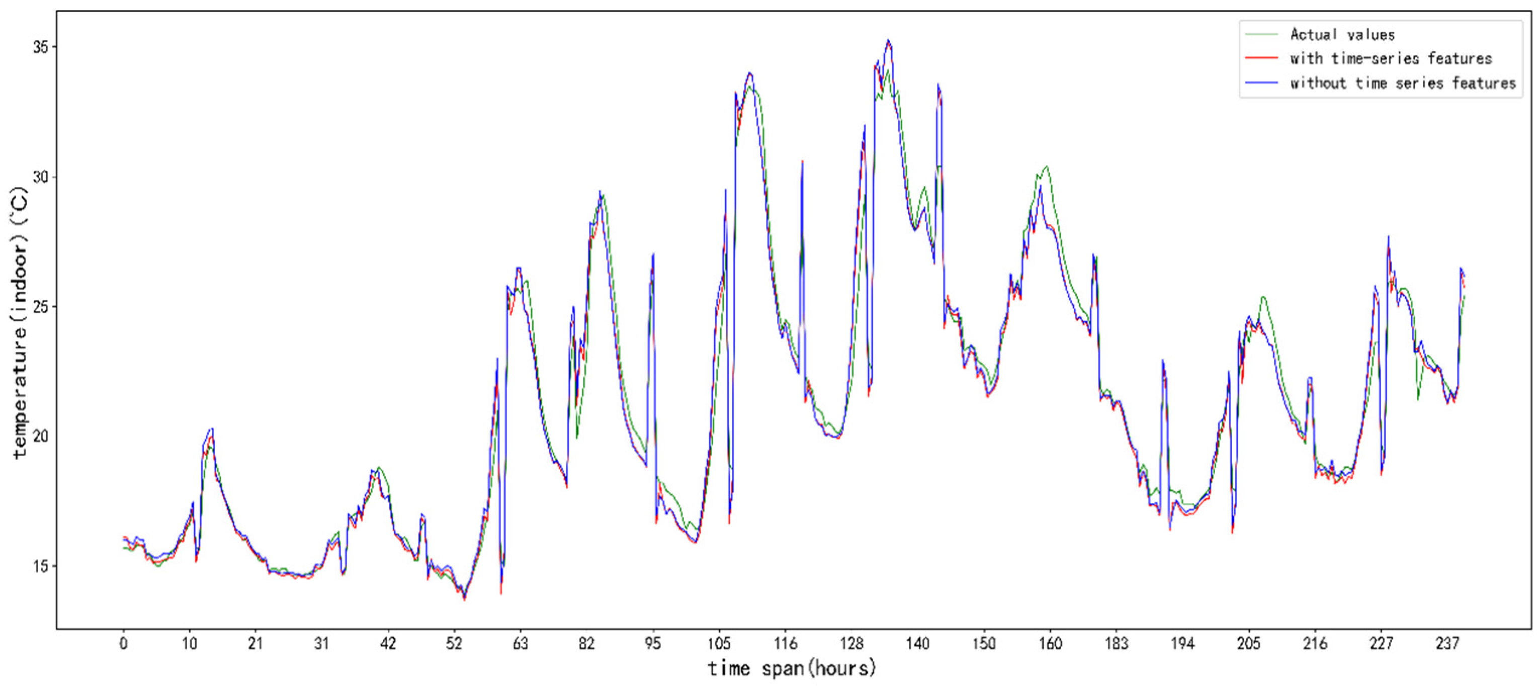
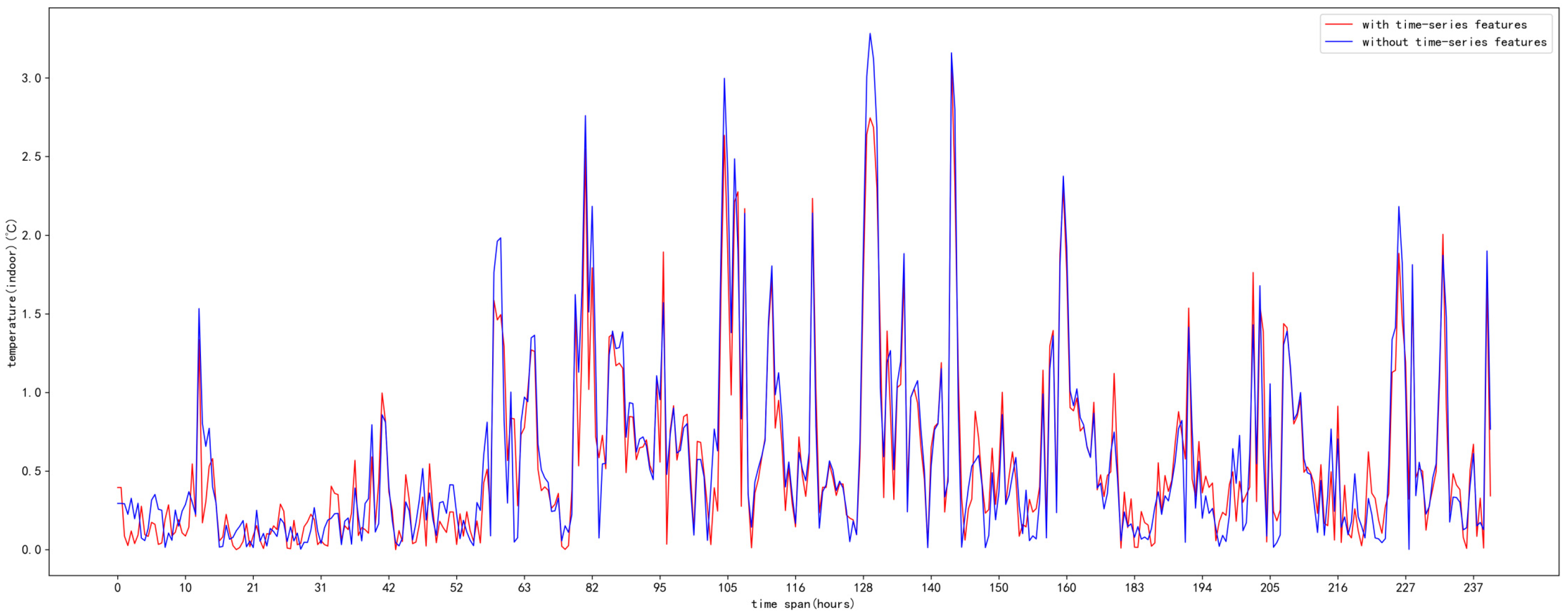
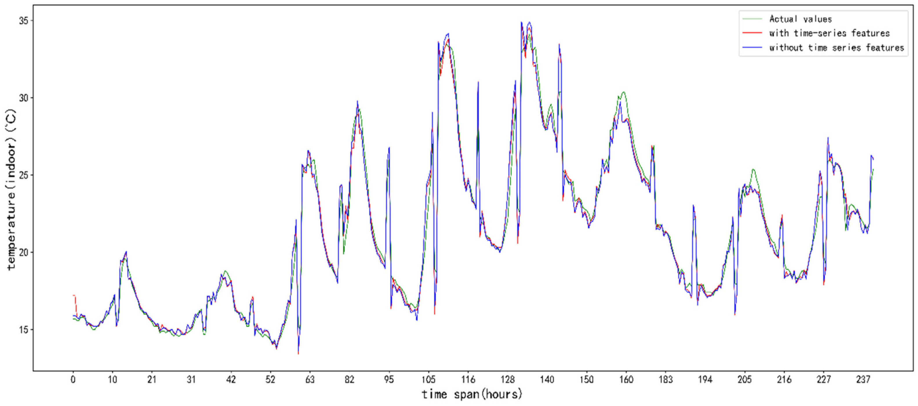
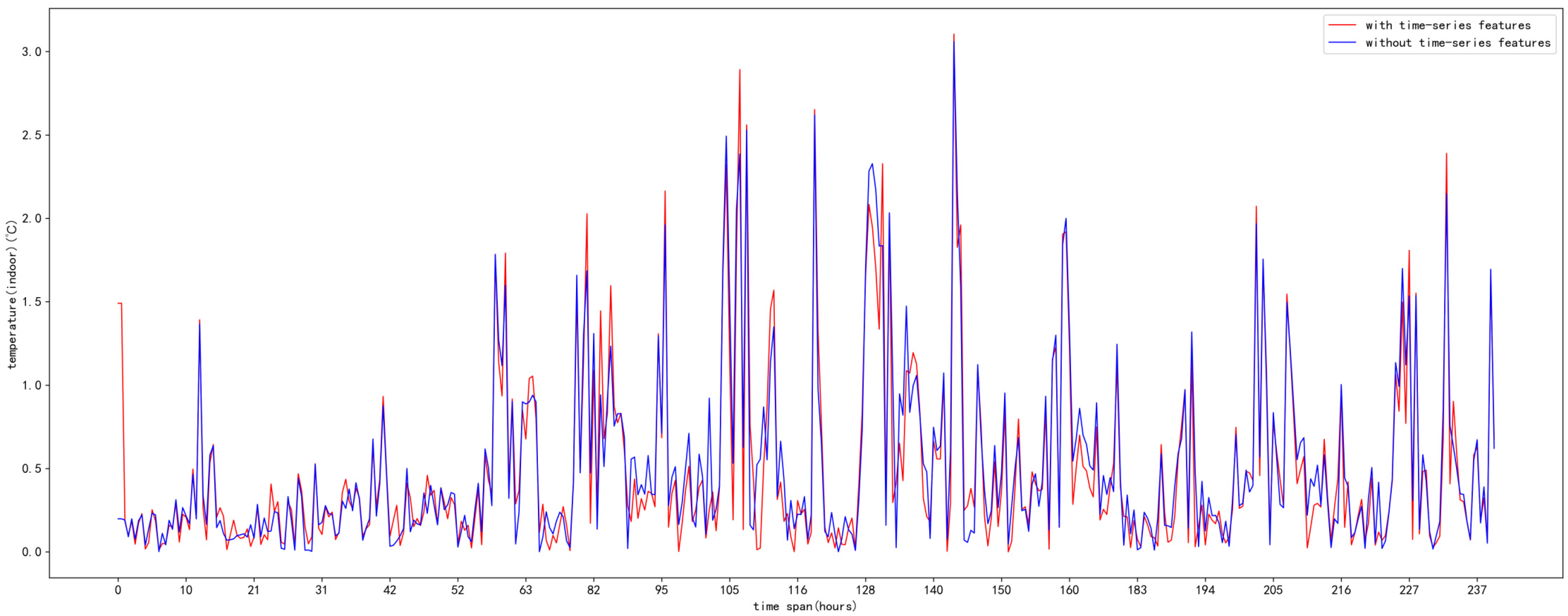
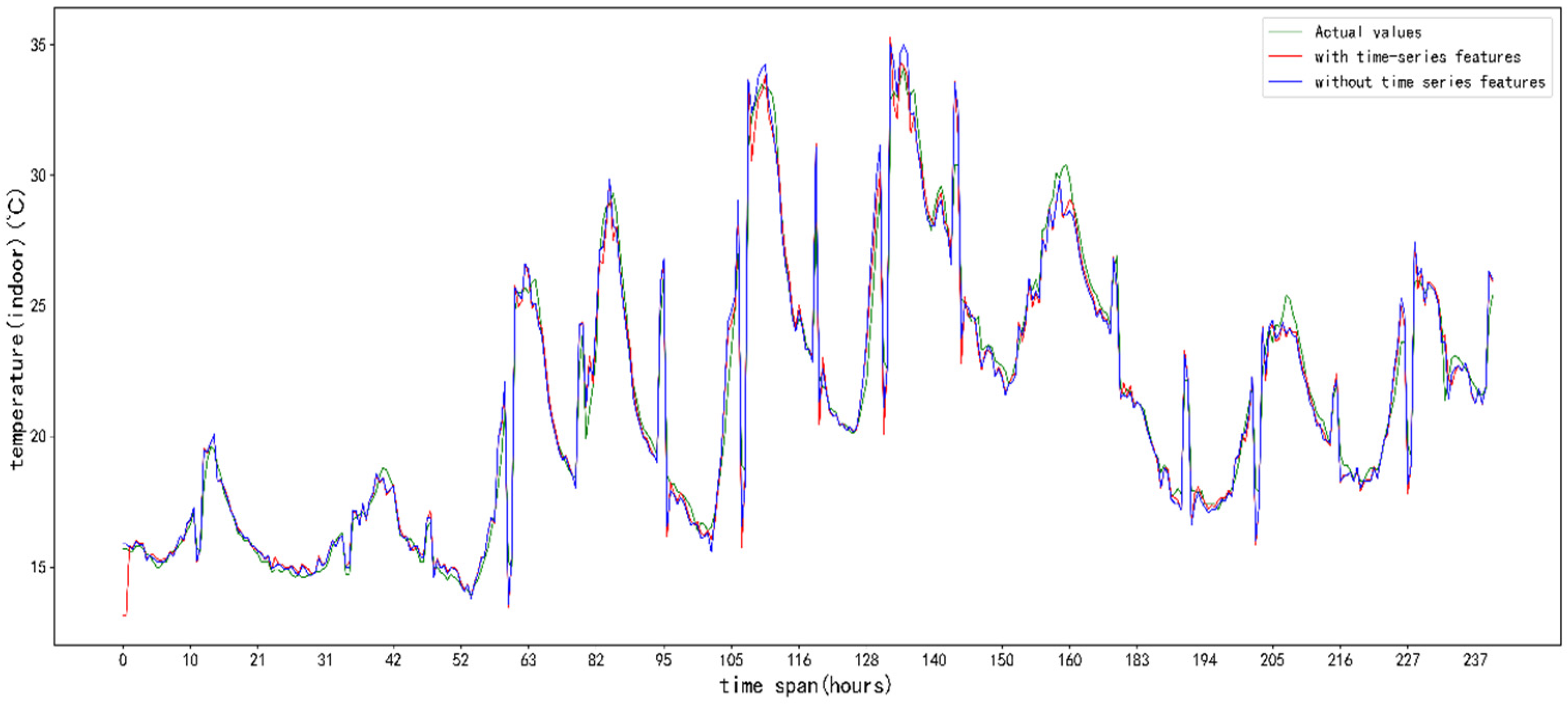
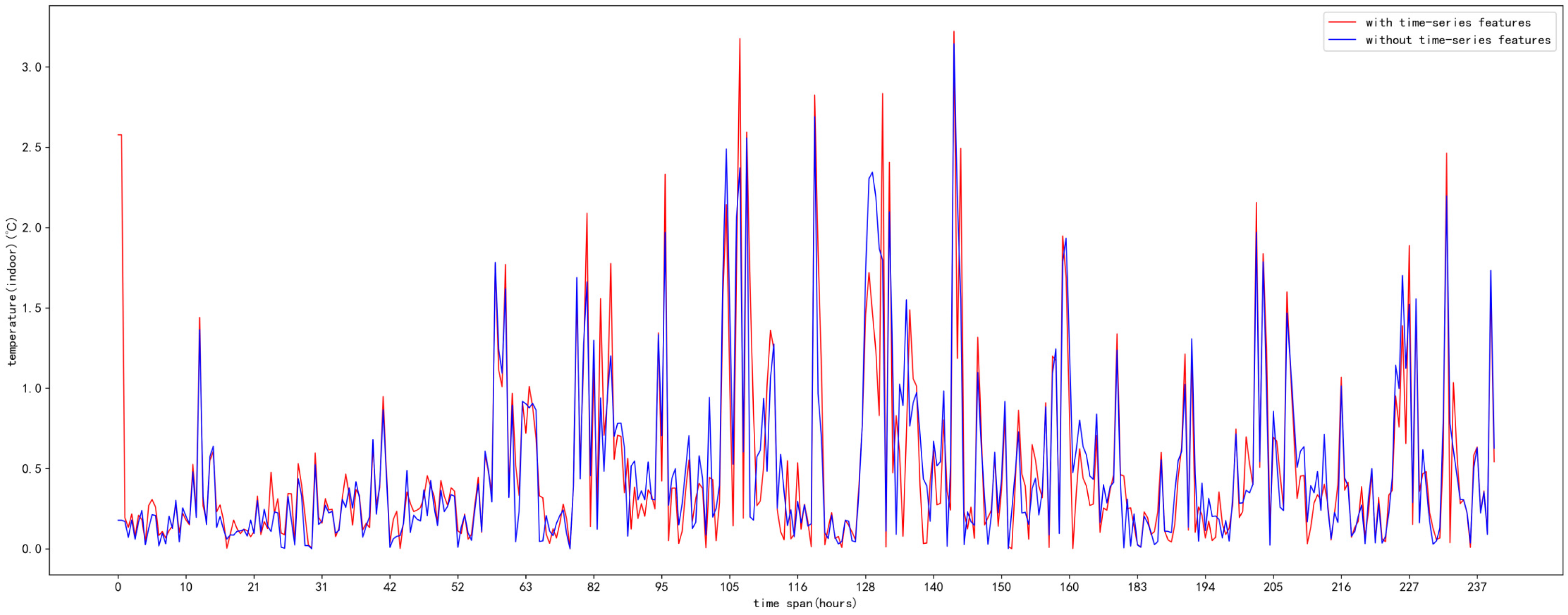
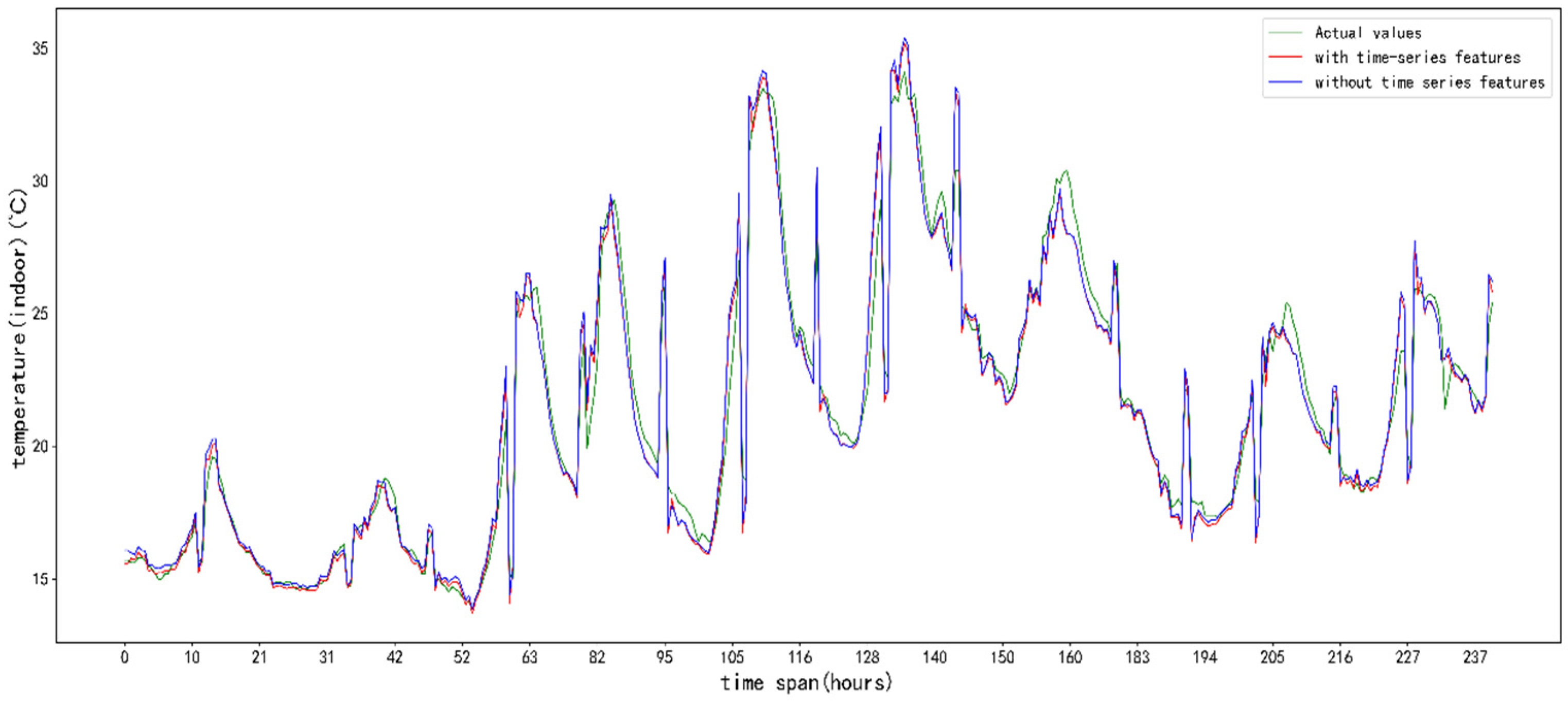
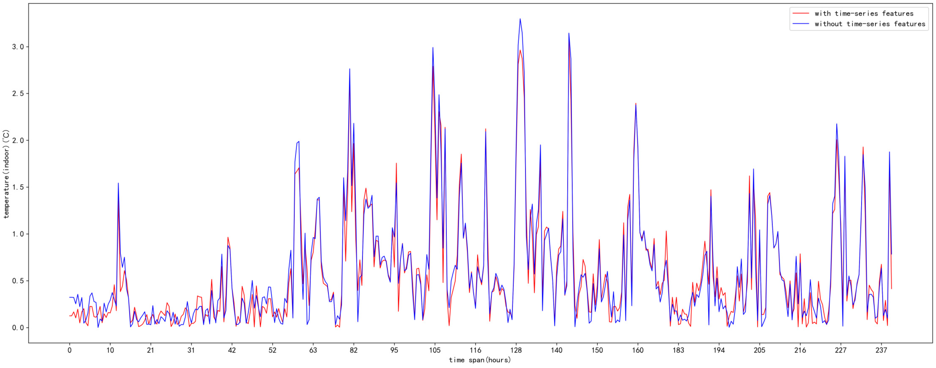
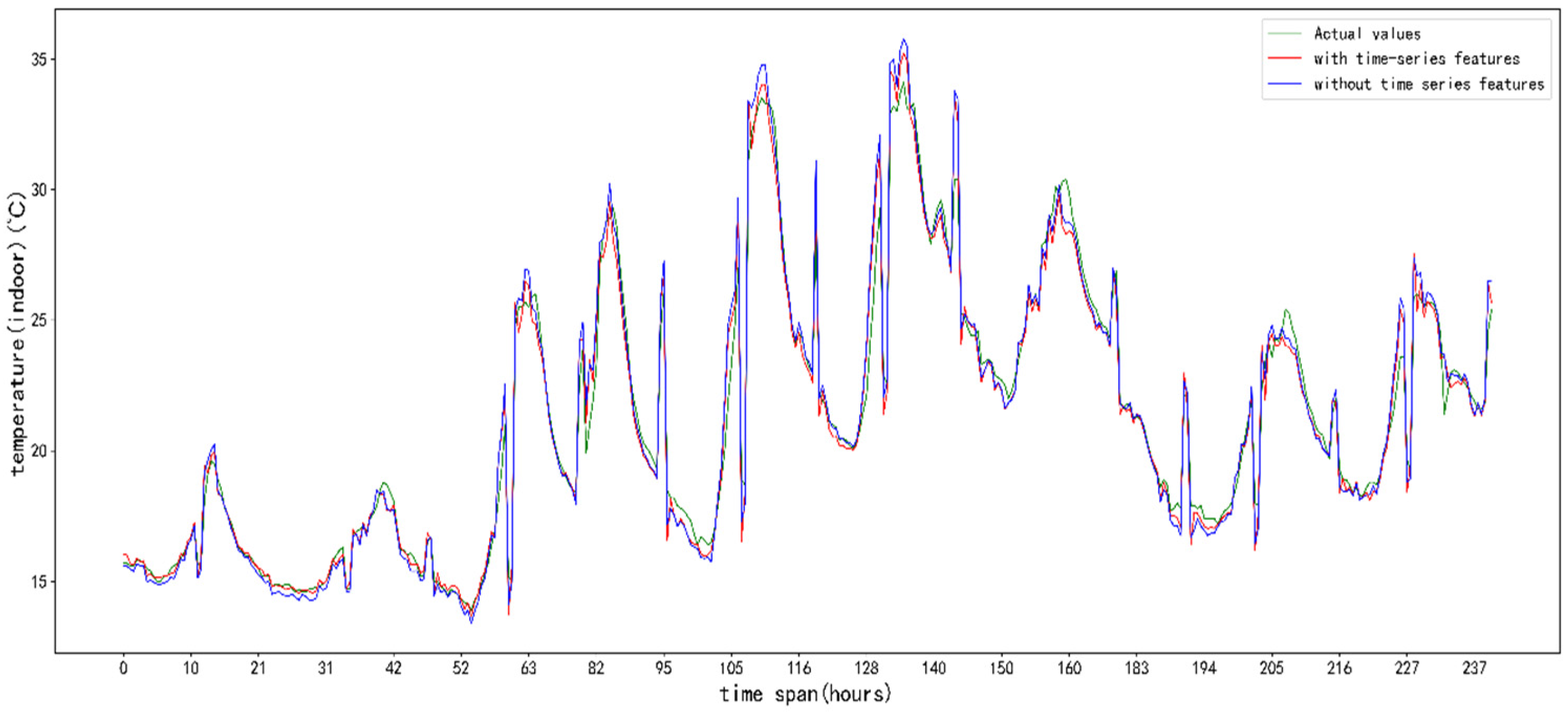
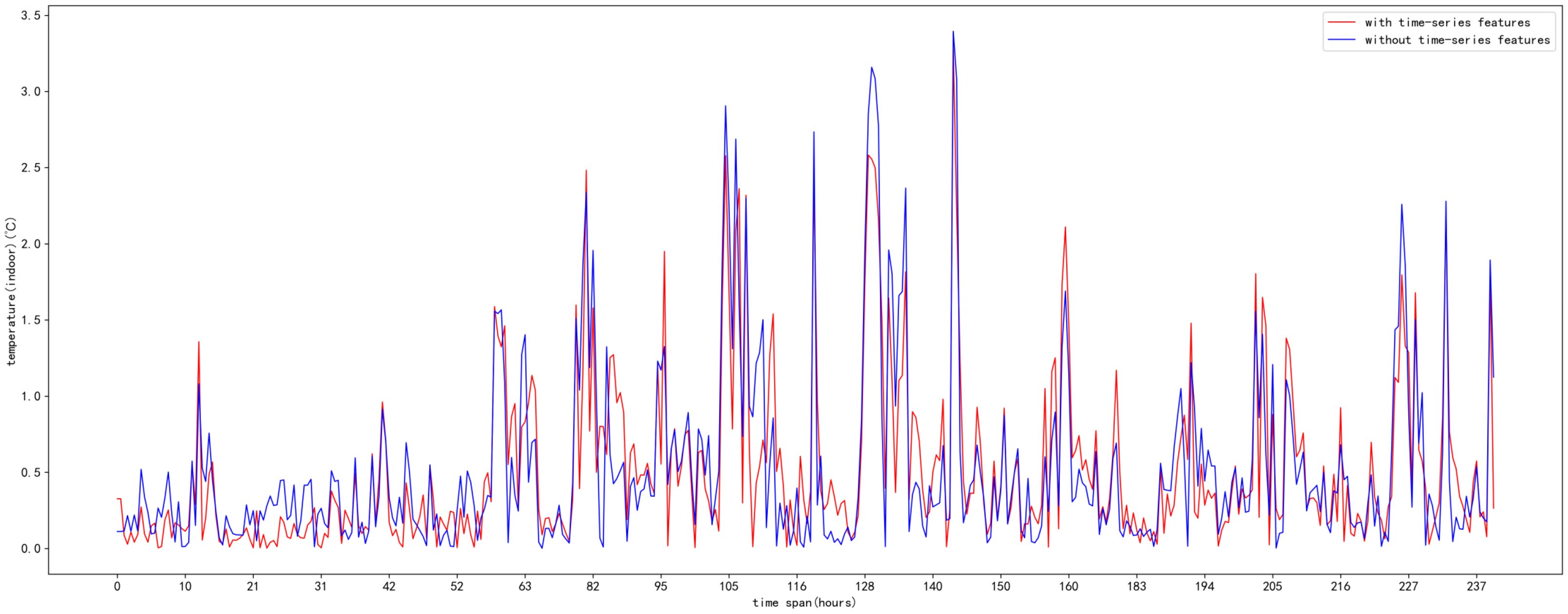
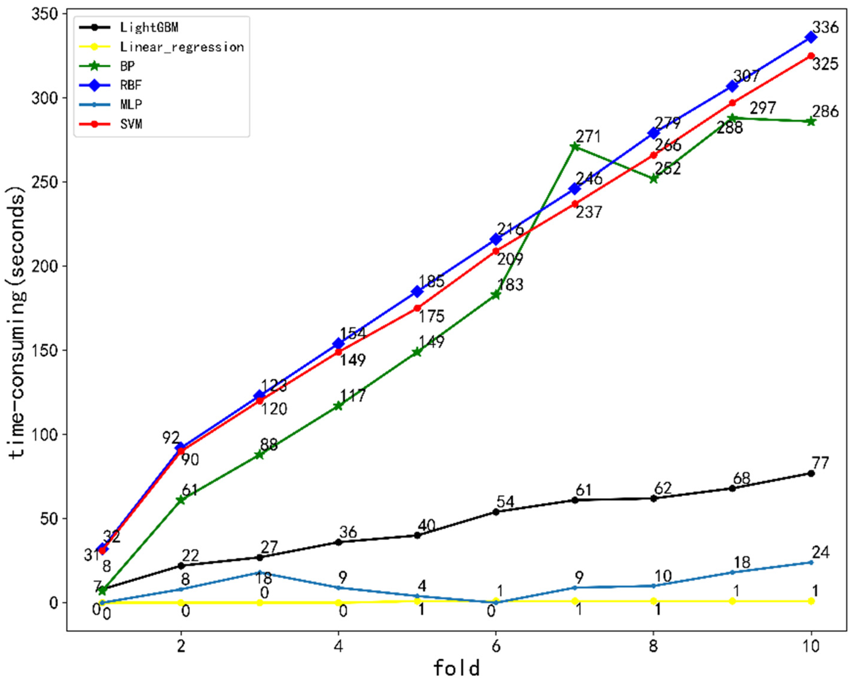
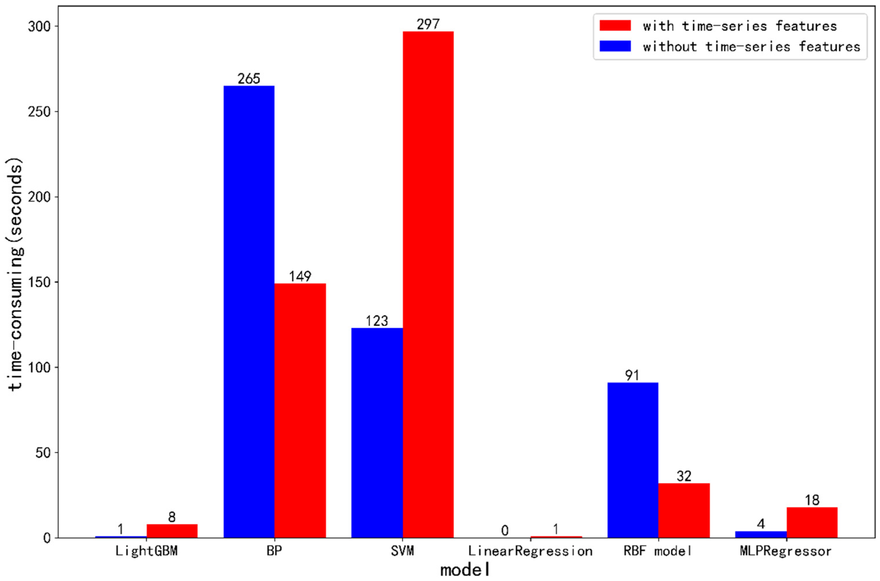
5. Results and Analysis

5.1. Evaluation Indicator

In quantitatively evaluating differences in the fitting degree between models and between original features and time-series features, the mean square error (MSE), mean absolute error (MAE), and R-square coefficient of determination (R²) were used as evaluation indicators to quantitatively distinguish and compare the prediction results of each model. The formulas for calculating the evaluation indicator are:

$$\mathrm{MSE}(y,y^{^})=\frac{1}{n}{\sum }_{i=0}^{n-1}{(y_i-y_i^{^})}^2,$$

(15)

$$\mathrm{MAE}(y,y^{^})=\frac{1}{n}{\sum }_{i=0}^{n-1}|y_i-y_i^{^}|,$$

(16)

$$R^2\left(y,y^{^}\right)=1-\frac{{\sum }_{i=0}^{n-1}{(y_i-y_i^{^})}^2}{{\sum }_{i=0}^{n-1}{(y_i-y^{-})}^2},$$

(17)

where $y_i$ is the actual value and $y_i^{^}$ is the predicted value of the $i$-th group of performance evaluation data, $y^{-}$ is the average value of data, and n is the total number of samples. MSE and MAE, respectively, denote the MSE and MAE of the predicted value and actual value. A smaller index value indicates a better prediction. The R² coefficient of determination indicates the degree of fitting between the predicted value and the actual value.

5.2. Hyperparameter Selection

The hyperparameters of a model are generally determined by cross-validation so that the model performs better on new data [34]. Since the experimental data in this paper are time-series data and there is a strict time-series relationship between the training set and the test set, the premise of the traditional cross-validation method is that the samples are independent and identically distributed [35]. Time-series data contain information such as that of the periodicity and the relationship between past and future data in the change process. This situation does not meet the basic assumption of independent and identically distributed data in cross-validation, and the cross-validation method based on time series should thus be adopted. Commonly used timing-based cross-verification methods [36,37] are the blocked cross-validation [38] procedure, which is similar to standard cross-validation, hv-blocked cross-validation proposed by Racine [39], which extends blocked cross-validation to further increase the independence among observations, and the modified cross-validation procedure [40], which removes observations from the training set that are correlated with the test. Vitor Cerqueira et al. compared and analyzed all the cross-validation methods for time series [41]. Based on their results, blocked cross-validation was used in the present study to determine hyperparameters.

5.3. Analysis of Results

We used the Python language for programming and extracted the difference features, statistical features, and cross-features mentioned above. The LightGBM model, BP neural network, SVM, linear regression model, RBF neural network, and multiple linear regression (MLPRegressor, MLP) were used for training and prediction. The dataset was split 1- to 10-fold to validate the selection of the best hyperparameters and retrain all the models. The fitting results of the models are shown in Figure 5, Figure 6, Figure 7, Figure 8, Figure 9, Figure 10, Figure 11, Figure 12, Figure 13, Figure 14, Figure 15 and Figure 16. The green line shows real values of the test set data, and the red and blue lines show the prediction results of each model on the test set. The figures show that each model performed well in terms of the degree of fitting, and the fitting result of LightGBM was better than the fitting results of the other five models, being closer to the trend line of the actual value. Since the temperature in the greenhouse has a strong time sequence (i.e., without the effects of special factors), the greenhouse temperature at this time strongly correlated with the greenhouse temperature at the previous time. The fitting of the predicted value to the actual value in the early stage was better than that in the later stage. The value on the horizontal axis is the number of hours after 1:00 on 3 April 2019.

In Figure 5, the green line is the change curve of the real value, the blue line is the change curve of the prediction result of LightGBM using the original features, and the red line is the change curve of the prediction result of LightGBM after adding the time-series features. It is seen that when the temperature smoothly changed, the prediction results were close to the real value both before and after adding the time-series features. When the temperature sharply changed, the prediction result was closer to the curve of the real data after adding the time-series features. The situation was similar at other positions where the temperature suddenly changed on the curve, such as approximately 160 and 183 h.

In Figure 6, the blue line is the absolute error of the prediction results without time-series features, and the red line is the absolute error of the prediction results after adding time-series features. It is seen that in the early prediction results, the results obtained using only the original features and those also using the time-series features were close, but after approximately 52 h, the absolute error when using only the original features gradually became greater than that when also using the time-series features. The statistical analysis of the results in Figure 6 reveals that the mean value of the absolute error when using only the original features was 0.5177 °C, and the standard deviation of the absolute error was 0.5652 °C. The mean value of the absolute error when also using the time-series features was 0.4491 °C, and the standard deviation of the absolute error was 0.5259 °C. The mean value and standard deviation of the absolute error when also using the time-series features were less than those when using only the original features, and the prediction result obtained when also using the time-series features was closer to the real value than that obtained using only the original features, and the fluctuation of the error was smaller.

Figure 7 and Figure 8 show that when the temperature trend changed (i.e., from decreasing to increasing or from increasing to decreasing), the prediction results of the BP neural network had lower absolute errors after time-series features were added. Statistical analysis of the results in Figure 8 revealed that the mean value and standard deviation of the absolute error were 0.5852 and 0.6146 °C, when using only the original features, and 0.5617 and 0.5640 °C when also using the time-series features. Therefore, the prediction result of the BP neural network when also using the time-series features was better than that when using only the original features, but worse than that of LightGBM.

The prediction results and absolute errors of the SVM model are shown in Figure 9 and Figure 10. Statistical analysis of the results in Figure 10 showed that the mean value and standard deviation of the absolute error of the SVM model were 0.5111 and 0.5374 °C, when using only the original features, and 0.4917 and 0.5476 °C when also using the time-series features. Therefore, the prediction result of the SVM when also using time-series features was better than that when using only the original features, but the error fluctuation was larger, and it was better than that of the BP neural network with time-series features but worse than that of LightGBM.

The prediction results and absolute errors of linear regression model are shown in Figure 11 and Figure 12. Statistical analysis of the results in Figure 12 showed that the mean value of the absolute error of linear regression when using only the original features was 0.4988 °C, and the standard deviation of the absolute error was 0.5414 °C. The mean value of the absolute error when also using the time-series features was 0.5030 °C, and the standard deviation of the absolute error was 0.5732 °C. In contrast with the prediction results of the previous model, the mean value and standard deviation of the absolute error in the prediction results of the linear regression model increased after adding the time-series features. The ability of linear regression to distinguish the time-series features is thus not strong, which relates to the characteristics of the linear regression model itself.

The degree of fitting of the prediction curve and the real curve in Figure 13 and the fluctuation of the absolute error in Figure 14 reveal that the absolute error in the prediction result of the time-series features of the RBF model was lower than that of other models approximately 52 h previous, but the error in the subsequent results was similar to that of the prediction result using the original features and worse than that of other models. The RBF model has better recognition ability for short-term time-series features but poor recognition ability for long-term time-series features. Statistical analysis of the results in Figure 14 shows that the mean value and standard deviation of the absolute error were 0.5901 and 0.6148 °C for the original features only and 0.5749 and 0.5867 °C for the time-series features also. The accuracy of the prediction results and the fluctuation of errors were worse for the RBF model than the previous models.

The prediction results and absolute errors of the MLP model are shown in Figure 15 and Figure 16. Statistical analysis of the results in Figure 16 showed that the maximum, mean, and standard deviation of the absolute error were 3.3944, 0.5229, and 0.6028 °C, respectively, for the original features only, and 3.2793, 0.5141, and 0.5583 °C, respectively, for the time-series features also. In the same way, when time-series features were added to the MLP model, not only the mean absolute error of the prediction results but also the fluctuation of the error decreased.

Table 3. Statistical analysis of the absolute error with and without time-series features.

	Indicators	Without Time-Series Features			With Time-Series Features
Model		Max	Mean	SD	Max	Mean	SD
LightGBM		3.0942	0.5177	0.5652	2.7378	0.4491	0.5259
BP		3.2832	0.5852	0.6146	3.1263	0.5617	0.5640
SVM		3.0594	0.5111	0.5374	3.1045	0.4917	0.5476
Linear Regression		3.1440	0.4988	0.5414	3.2217	0.5030	0.5732
RBF		3.2983	0.5901	0.6148	3.0887	0.5749	0.5867
MLP		3.3944	0.5229	0.6028	3.2793	0.5141	0.5583

compares the prediction of each model before and after adding the time-series features against the real value and presents a simple statistical analysis of the absolute error of each model.

Table 3 shows that LightGBM saw the most obvious improvement after the addition of time-series features. Not only the maximum error but also the mean error and the standard deviation of the error in the prediction results were the smallest. Therefore, in general, LightGBM made the best and most stable predictions among the models.

Figure 5, Figure 6, Figure 7, Figure 8, Figure 9, Figure 10, Figure 11, Figure 12, Figure 13, Figure 14, Figure 15 and Figure 16 compared the prediction results of each model at each time point with the real results. Good and poor results were intuitively seen in all the predictions. We conducted a quantitative analysis of the prediction results of each model. Using Equations (15)–(17), blocked cross-verification was adopted to adjust the hyperparameters of each model, and all models were trained with the optimal parameters obtained by verification. The evaluation indicators of the prediction results of each model with and without time-series features are presented in

Table 4. Evaluation indicators of the models before and after adding time-series features.

	Indicators	Without Time-Series Features			With Time-Series Features			(MSE1i-MSE2i)/ MSE1i	(MSE2i-MSE2LightGBM)/MSE2i
Model		MSE1	MAE2	R2_score1	MSE2	MAE2	R2_score2
LightGBM		0.5868	0.5177	0.9760	0.4776	0.4491	0.9805	18.61%	-
BP		0.7193	0.5852	0.9706	0.6329	0.5617	0.9742	12.01%	24.54%
SVM		0.5494	0.5111	0.9776	0.5409	0.4917	0.9779	1.55%	11.70%
Linear Regression		0.5413	0.4988	0.9779	0.5808	0.5030	0.9763	−7.30%	17.77%
RBF		0.7254	0.5901	0.9704	0.6739	0.5749	0.9725	7.10%	29.13%
MLP		0.6360	0.5229	0.9740	0.5753	0.5141	0.9765	9.54%	16.98%

.

Table 4 shows that all indicators were best for linear regression before time-series features were involved, followed by the SVM model and the RBF model. After adding time-series features, the indicators of the LightGBM model were the best, whereas those of the RBF model remained the worst. However, the MSE was reduced by 7.10%, the MAE was reduced by 2.58%, and the R2_Score was reduced by 0.22% with the inclusion of time-series features for the RBF model.

A comparison of the indicators before and after the inclusion of time-series features in all models revealed that, for the prediction results with time-series features, except those of the linear regression model, the indicators have improved. Among them, the indicators of the LightGBM model improved the most, with the MSE decreasing by 18.60%, the MAE decreasing by 13.25%, and the R2_score increasing by 0.45%. All indicators of LightGBM were the best among the several models. This is because the LightGBM model is based on the decision tree model, and the result is the average result after the accumulation of multiple tree models. This characteristic can weaken the effect of abnormal data, and the recognition of the complex features constructed in this paper is the same as that of the original features, which are divided into branches depending on the optimal threshold value.

The MSE, MAE, and R2_score of the sub-optimal SVM model decreased by 1.55% and 3.80% and increased by 0.03% after adding the time-series features. The SVM model can specify different kernel functions in the decision function, and the transformation can be nonlinear (i.e., the transformation space can be high-dimensional), such that its input space can be nonlinear, which is of great help in the recognition of high-dimensional complex features. Therefore, the SVM can still achieve excellent performance after adding time-series features. Both BP and RBF neural network models have the ability of multi-dimensional nonlinear mapping, self-learning, and self-adaptation, such that they can also identify high-dimensional complex features. Since each model has a different base learner and recognition ability for high-dimensional complex features, the time-series information that each model can recognize is also different to some extent. The prediction effect can thus be improved by adding time-series features.

Owing to the shortcomings of the linear regression model, it is difficult to model nonlinear data or features with correlation and to identify highly complex features well. Therefore, the difference features, statistical features, and combination features mentioned in this paper do not perform well in the linear regression model. Compared with linear regression, the MLP model can fit nonlinear data and deal with complex relationships more flexibly. Therefore, the MLP model can better identify the complex features constructed in this paper, and the prediction indicators of the MLP model have been greatly improved after the addition of time-series features. Compared with the predication without time-series features, the MSE decreased by 9.54%, the MAE decreased by 1.68%, and the R2_score increased by 0.26%.

In summary, Table 4 shows that the prediction of each model was improved after adding time-series features, and the time-series features made the most obvious improvements to the prediction of LightGBM, with the MSE on the test set decreasing from 0.5868 to 0.4776 (i.e., by 18.61%). LightGBM performed better than the other models for all evaluation indicators. After adding the time-series features, the fitting degree of LightGBM was 98.05%. Comparing LightGBM with other models after adding time-series features, the MSE was lower by 11.70% (versus the SVM) and −29.12% (versus the RBF), the MAE was lower by 8.66% (versus the SVM) and −21.88% (versus the RBF), and the R2_score was improved by 0.26% (versus the SVM) and 0.80% (versus the RBF). LightGBM therefore performed better in prediction.

We statistically analyzed the confidence interval of the absolute error between the predicted value and the real value of each model at the 95% confidence level, and the results are presented in

Table 5. Confidence interval of each model at the 95% confidence level.

	0.95 Confidence Interval	Without Time-Series Features	With Time-Series Features
Model
LightGBM		[−0.5901, 1.6256]	[−0.5816, 1.4799]
BP		[−0.6194, 1.7898]	[−0.5436, 1.6672]
SVM		[−0.5422, 1.5645]	[−0.5815, 1.5650]
Linear Regression		[−0.5624, 1.5601]	[−0.6204, 1.6266]
RBF		[−0.6150, 1.7952]	[−0.5750, 1.7249]
MLP		[−0.6586, 1.7045]	[−0.5801, 1.6085]

. The table shows that for the same confidence level and the same sample size, the confidence interval of the absolute value error of the predicted value of the LightGBM model with time-series features was narrower than the intervals for other models, which shows that the estimated error for the LightGBM model was smaller and the prediction was more accurate than for the other models. The confidence intervals of the linear regression model and SVM model without time-series features were smaller than the interval for the time-series model. The results here coincide with the results presented in Table 4. After adding the features of the time series, BP neural network, and RBF neural network, the confidence interval decreased to a certain extent, but the effect was weaker than that for the LightGBM model.

Figure 17 shows the variation in the training time for each model with the cross-validation folding number. A greater number of folds for cross-validation results in a longer time for training. Among the models, the training times of the BP neural network and MLP model had a negative increase with the change in fold number, owing to the early stopping mechanism used to prevent overfitting in the experimental process. This also shows the instability of using the BP neural network and MLP in cross-verification. Compared with the RBF model, SVM, and BP neural network, the LightGBM model required less training time and obtained better results in less time. The LightGBM model is thus superior to other models in terms of both prediction accuracy and time efficiency.

Figure 18 compares the training times for different models with the optimal hyperparameters before and after adding time-series features. The BP neural network and RBF model required less training time after adding time-series features because the early stopping mechanism ensures that the parameters of the model converge earlier. The time required by the SVM model obviously increased after adding the time-series features, which indicates that the SVM model is extremely sensitive to the feature dimension. Compared with the other models, LightGBM took a little more time than the linear regression and much less time than other models after adding time-series features. LightGBM thus rapidly provided prediction results.

6. Discussion

In this paper, we extracted the time-series features of the factors affecting the indoor temperature in a greenhouse and then used the LightGBM model to more accurately predict the greenhouse temperature. It was found in the experiment that linear regression did not have a strong ability to identify high-dimensional complex features, and therefore its MSE and MAE for prediction did not decrease with the inclusion of time-series features. Indeed, the original feature prediction performance was better. The combination of the LightGBM model and time-series features greatly improved the accuracy of prediction results. Although models other than the linear regression model have improved the prediction performance after adding time-series features, the positive effect on the performance of the LightGBM model was more obvious. In terms of the required training time, following cross-validation, the training time required for most models is directly proportional to the number of cross-validation folds, and the proportionality coefficient of the LightGBM model was relatively moderate. Although the LightGBM model was not the fastest, it obtained the optimal results in a relatively short time.

Owing to the limitation that the training data provided by the competition platform are only for March and April, the method proposed in this paper has not been verified using data for other periods, and we have checked relevant works published in the past two years and have not found any other study using this dataset. Therefore, there is no comparison between presented results and the results from the existing literature that deals with similar research. Moreover, the limited original feature information in the training data limited the time-series feature information that we could extract, such that some factors affecting the greenhouse temperature were not considered. If other quarterly data are added and the volume of data is sufficient, because the LightGBM model is based on the GBDT algorithm, the temperature corresponding to different quarters will be divided into different branches when building the boosting tree. In addition, if more influencing factors such as the light intensity and carbon dioxide concentration are added, more information can be extracted during time-series feature construction. Therefore, if the data of different quarters are taken as input, theoretically, the model can also learn the time-series information of different quarters.

Time-series cross-validation is highly dependent on the ability of the base learner of the model to recognize historical time-series information. Stronger recognition ability means that more information will be extracted with an increase in the number of time-series features; otherwise, less information will be extracted. Therefore, when the data used for cross-validation are divided into multiple folds, a greater number of folds results in each fold containing less historical information. In the case of a multi-fold partition, the model can extract different historical time-series information from the data of each fold, which leads to a difference in the prediction results. A slight difference can help the model adjust parameters and improve the model performance, while large differences will make the model unstable and worsen the prediction results.

7. Conclusions

Based on an analysis of environmental factors that affect the indoor temperature, we added difference features, statistical features, and other time-series characteristics of the temperature, humidity, and air pressure using cross-features as the input of the nonlinear relationship features and applying the LightGBM model, linear regression, SVM, BP neural network, RBF neural network, and MLPRegressor for predictive analysis. In comparative tests using only the original features and adding time-series features, we found that, after adding time-series features, the prediction results of LightGBM were better than those of the other models, which revealed that LightGBM has better adaptability to time-series features. Compared with the LightGBM model, linear regression does not have strong recognition ability for time-series features. Therefore, applying time-series features to linear regression does not help to identify high-dimensional complex feature information. Compared with the SVM, BP neural network, and RBF neural network, LightGBM took less time in the training process and did not easily fall into a local optimum. Compared with the dynamic model and MLPRegressor mentioned in the literature [10,11], LightGBM is not limited to small ecosystems but is applicable to other situations. Furthermore, LightGBM had the smallest mean value and standard deviation of the absolute error, indicating that LightGBM made the most stable prediction among the various models.

It is therefore concluded that the greenhouse temperature prediction model based on time-series features and LightGBM not only trains the model in a shorter time but also more accurately predicts the greenhouse temperature.

The growth of crops is strongly dependent on aspects of the natural environment, such as light, temperature, humidity, and air pressure, which affect the crop yield and quality. In the growth cycle of crops, all kinds of chemical reactions need to occur within the crop material at an appropriate temperature, and therefore temperature is often the decisive factor of crop growth and development. The LightGBM prediction results are important reference values for greenhouse temperature control and play an important role in improving the crop yield and quality and promoting the development of smart agriculture.

Owing to the limitation of data samples, the reported experiment has not been verified on other datasets outside the dataset for 2019 used in the present study. Future work will obtain more complete original data affecting the greenhouse temperature for further testing of the model and expanding the use scenario.

References

1. Wang, X.; Luo, J.; Li, X. Study on Temperature and Humidity Prediction Model of Plastic Greenhouse Environment. Water Sav. Irrig. 2013, 10, 23–26. [Google Scholar]
2. Li, Y.; Wu, D.; Yu, Z. Simulation and Test Research of Micrometeorology Environment in a Sun-Light Greenhouse. Trans. Chin. Soc. Agric. Eng. 1994, 1, 130–136. [Google Scholar]
3. Cui, L.; Bian, Z. Temperature Prediction Model Based on Improved Support Vector Machine. Technol. Innov. Appl. 2020, 10, 101–102. [Google Scholar]
4. Peng, X.; Bai, B.; Wang, F.; Zhou, G. Layout of Environmental Science Data Monitoring Sensors in Sunlight Greenhouse. Jiangsu Agric. Sci. 2017, 45, 167–170. [Google Scholar]
5. Shi, Y.; Guo, Q.; Xu, C. Temperature Field Analysis of Greenhouse Based on Moving Least Square Method. Agric. Res. Appl. 2015, 2, 37–41. [Google Scholar]
6. Yu, C.; Wang, J.; Ying, Y. Greenhouse Temperature Prediction Model Based on Radial Basias Function Neural Networks. J. Biomath. 2006, 4, 549–553. [Google Scholar]
7. Shen, C.; Yang, J. RBF Neural Network PID Control for Greenhouse Temperature Control System. Control Eng. China 2017, 24, 361–364. [Google Scholar]
8. Zhang, K.; Zhao, K. Greenhouse Temperature Prediction Based on Improved CFA PSO-RBF Neural Network. Comput. Appl. Softw. 2020, 37, 95–99. [Google Scholar]
9. Xia, S.; Li, L. Application of Greenhouse Temperature Prediction Based on PSO-RBF Neutral Network. Comput. Eng. Des. 2017, 38, 744–748. [Google Scholar]
10. Mohammadi, B.; Ranjbar, S.F.; Ajabshirchi, Y. Application of dynamic model to predict some inside environment variables in a semi-solar greenhouse. Inf. Process. Agric. 2018, 5, 279–288. [Google Scholar] [CrossRef]
11. Nguyen-Xuan, S.; Nhat, N.L. A dynamic model for temperature prediction in glass greenhouse. In Proceedings of the 2019 6th NAFOSTED Conference on Information and Computer Science (NICS), Hanoi, Vietnam, 12–13 December 2019; pp. 274–278. [Google Scholar]
12. Li, X.; Zhang, X.; Wang, Y.; Zhang, K.; Chen, Y.-F. Temperature prediction model for solar greenhouse based on improved BP neural network. J. Phys. Conf. Ser. 2020, 1639, 012036. [Google Scholar] [CrossRef]
13. Zhao, H.; Shi, L.R.; Wang, H.J. Sunlight Greenhouse Temperature Prediction Model Based on Bayesian Regularization BP Neural Network. Appl. Mech. Mater. 2015, 740, 871–874. [Google Scholar] [CrossRef]
14. Papacharalampous, G.; Tyralis, H.; Papalexiou, S.M.; Langousis, A.; Khatami, S.; Volpi, E.; Grimaldi, S. Global-scale massive feature extraction from monthly hydroclimatic time series: Statistical characterizations, spatial patterns and hydrological similarity. Sci. Total Environ. 2021, 767, 144612. [Google Scholar] [CrossRef] [PubMed]
15. Jia, Z.; Lin, Y.; Liu, Y.; Jiao, Z.; Wang, J. Refined nonuniform embedding for coupling detection in multivariate time series. Phys. Rev. E 2020, 101, 062113. [Google Scholar] [CrossRef] [PubMed]
16. Jia, Z.; Lin, Y.; Jiao, Z.; Ma, Y.; Wang, J. Detecting causality in multivariate time series via non-uniform embedding. Entropy 2019, 21, 1233. [Google Scholar] [CrossRef] [Green Version]
17. Li, H. Statistic Learning Method, 2nd ed.; Tsinghua University Press: Beijing, China, 2019. [Google Scholar]
18. Learn, S. Ensemble Methods—Gradient Boosting. 2019. Available online: https://scikit-learn.org/stable/modules/ensemble.html#gradient-tree-boosting (accessed on 1 July 2022).
19. Chen, T.; Guestrin, C. Xgboost: A scalable tree boosting system. In Proceedings of the 22nd ACM SIGKDD International Conference on Knowledge Discovery and Data Mining, Ser. KDD’16, San Francisco, CA, USA, 13–17 August 2016; ACM: New York, NY, USA, 2016; pp. 785–794. [Google Scholar]
20. Ke, G.; Meng, Q.; Finley, T.; Wang, T.; Chen, W.; Ma, W.; Ye, Q.; Liu, T.-Y. Lightgbm: A highly efficient gradient boosting decision tree. In Advances in Neural Information Processing Systems 30; Guyon, I., Luxburg, U.V., Bengio, S., Wallach, H., Fergus, R., Vishwanathan, S., Garnett, R., Eds.; Curran Associates, Inc.: Red Hook, NY, USA, 2017; pp. 3146–3154. [Google Scholar]
21. Leevy, J.L.; Hancock, J.; Zuech, R.; Khoshgoftaar, T.M. Detecting Cybersecurity Attacks Using Different Network Features with LightGBM and XGBoost Learners. In Proceedings of the 2020 IEEE Second International Conference on Cognitive Machine Intelligence (CogMI), Atlanta, GA, USA, 28–31 October 2020; pp. 190–197. [Google Scholar] [CrossRef]
22. Xia, H.; Wei, X.; Gao, Y.; Lv, H. Traffic Prediction Based on Ensemble Machine Learning Strategies with Bagging and LightGBM. In Proceedings of the 2019 IEEE International Conference on Communications Workshops (ICC Workshops), Shanghai, China, 20–24 May 2019; pp. 1–6. [Google Scholar]
23. Machado, M.R.; Karray, S.; de Sousa, I.T. LightGBM: An Effective Decision Tree Gradient Boosting Method to Predict Customer Loyalty in the Finance Industry. In Proceedings of the 2019 14th International Conference on Computer Science & Education (ICCSE), Toronto, ON, Canada, 19–21 August 2019; pp. 1111–1116. [Google Scholar] [CrossRef]
24. Do, D.T.; Le, N.Q.K. Using extreme gradient boosting to identify origin of replication in Saccharomyces cerevisiae via hybrid features. Genomics 2020, 112, 2445–2451. [Google Scholar] [CrossRef]
25. Zhao, X.; Zhao, Q. Stock Prediction Using Optimized LightGBM Based on Cost Awareness. In Proceedings of the 2021 5th IEEE International Conference on Cybernetics (CYBCONF), Sendai, Japan, 8–10 June 2021; pp. 107–113. [Google Scholar] [CrossRef]
26. Mestre, G.; Portela, J.; Rice, G.; Roque, A.M.S.; Alonso, E. Functional time series model identification and diagnosis by means of auto- and partial autocorrelation analysis. Comput. Stat. Data Anal. 2021, 155, 107108. [Google Scholar] [CrossRef]
27. Kokoszka, P.; Rice, G.; Shang, H.L. Inference for the autocovariance of a functional time series under conditional heteroscedasticity. J. Multivar. Anal. 2017, 162, 32–50. [Google Scholar] [CrossRef] [Green Version]
28. Guan, B.; Zhao, Y.; Yin, Y.; Li, Y. A differential evolution based feature combination selection algorithm for high-dimensional data. Inf. Sci. 2021, 547, 870–886. [Google Scholar] [CrossRef]
29. Gu, J.; Mao, H. A Mathematical Model on Intelligent Control of Greenhouse Environment. Trans. Chin. Soc. Agric. Mach. 2001, 32, 63–65. [Google Scholar]
30. Yu, Q.; Huang, X.; Li, W.; Wang, C.; Chen, Y.; Ge, Y. Using Features Extracted From Vital Time Series for Early Prediction of Sepsis. In Proceedings of the 2019 Computing in Cardiology (CinC), Singapore, 8–11 September 2019; IEEE: Piscataway, NJ, USA, 2019; pp. 1–4. [Google Scholar] [CrossRef]
31. Li, Y.; Yang, C.; Sun, Y. Dynamic time features expanding and extracting method for prediction model of sintering process quality index. IEEE Trans. Ind. Inform. 2021, 18, 1737–1745. [Google Scholar] [CrossRef]
32. Shi, S. Temporal Characteristic of Climatic, Soil, and Hydrological Elements and Their Influencing Factors in The Upper Reaches of The Heihe River. Acta Geod. Cartogr. Sin. 2020, 49, 1508. [Google Scholar]
33. Tao, L.; Jeong, D.; Wang, J.; Adams, Z.; Bryan, P.; Levin, C.S. Simulation studies to understand sensitivity and timing characteristics of an optical property modulation-based radiation detection concept for PET. Phys. Med. Biol. 2020, 65, 215021. [Google Scholar] [CrossRef] [PubMed]
34. Varma, S.; Simon, R. Bias in error estimation when using cross-validation for model selection. BMC Bioinforma. 2006, 7, 1–8. [Google Scholar] [CrossRef] [PubMed] [Green Version]
35. Roberts, D.R.; Bahn, V.; Ciuti, S.; Boyce, M.S.; Elith, J.; Guillera-Arroita, G.; Hauenstein, S.; Lahoz-Monfort, J.J.; Schröder, B.; Thuiller, W.; et al. Cross-validation strategies for data with temporal, spatial, hierarchical, or phylogenetic structure. Ecography 2017, 40, 913–929. [Google Scholar] [CrossRef] [Green Version]
36. Bergmeir, C.; Hyndman, R.J.; Koo, B. A note on the validity of cross-validation for evaluating autoregressive time series prediction. Comput. Stat. Data Anal. 2018, 120, 70–83. [Google Scholar] [CrossRef]
37. Bergmeir, C.; Benítez, J.M. On the use of cross-validation for time series predictor evaluation. Inf. Sci. 2012, 191, 192–213. [Google Scholar] [CrossRef]
38. Snijders, T.A.B. On cross-validation for predictor evaluation in time series. In On Model Uncertainty and Its Statistical Implications; Springer: Berlin/Heidelberg, Germany, 1988; pp. 56–69. [Google Scholar]
39. Racine, J. Consistent cross-validatory model-selection for dependent data: Hv-block cross-validation. J. Econ. 2000, 99, 39–61. [Google Scholar] [CrossRef]
40. McQuarrie, A.D.; Tsai, C.-L. Regression and Time Series Model Selection; World Scientific: Singapore, 1998. [Google Scholar]
41. Cerqueira, V.; Torgo, L.; Smailović, J.; Mozetič, I. A comparative study of performance estimation methods for time series forecasting. In Proceedings of the 2017 IEEE international conference on data science and advanced analytics (DSAA), Tokyo, Japan, 19–21 October 2017; IEEE: Piscataway, NJ, USA, 2017; pp. 529–538. [Google Scholar]
Figure 1. Change in indoor air pressure with time before and after correction.
Applsci 13 01610 g001
Figure 2. Variation in the autocorrelation coefficient of the indoor temperature with order.
Applsci 13 01610 g002
Figure 3. Change in indoor temperature over time.
Applsci 13 01610 g003
Figure 4. Importance of each feature evaluated using the tree model.
Applsci 13 01610 g004
Figure 5. Fitting trend of the prediction results of LightGBM.
Applsci 13 01610 g005
Figure 6. Absolute error when using LightGBM with and without the time-series features.
Applsci 13 01610 g006
Figure 7. Fitting trend of the prediction results of the BP neural network.
Applsci 13 01610 g007
Figure 8. Absolute error of the BP neural network with and without the time-series features.
Applsci 13 01610 g008
Figure 9. Fitting trend of prediction results of the SVM.
Applsci 13 01610 g009
Figure 10. Absolute error of the SVM with and without the time-series features.
Applsci 13 01610 g010
Figure 11. Fitting trend of the prediction results of linear regression.
Applsci 13 01610 g011
Figure 12. Absolute error of the linear regression with and without the time-series features.
Applsci 13 01610 g012
Figure 13. Fitting trend of the prediction results of the RBF neural network.
Applsci 13 01610 g013
Figure 14. Absolute error of the RBF neural network with and without the time-series features.
Applsci 13 01610 g014
Figure 15. Fitting trend of the prediction results of the MLP model.
Applsci 13 01610 g015
Figure 16. Absolute error of the MLP model with and without the time-series features.
Applsci 13 01610 g016
Figure 17. Training time versus the number of folds of different models.
Applsci 13 01610 g017
Figure 18. Required training time with the optimal hyperparameters and with and without time-series features.
Applsci 13 01610 g018