
A Two-Phase Ensemble-Based Method for Predicting Learners’ Grade in MOOCs


Abstract
:1. Introduction
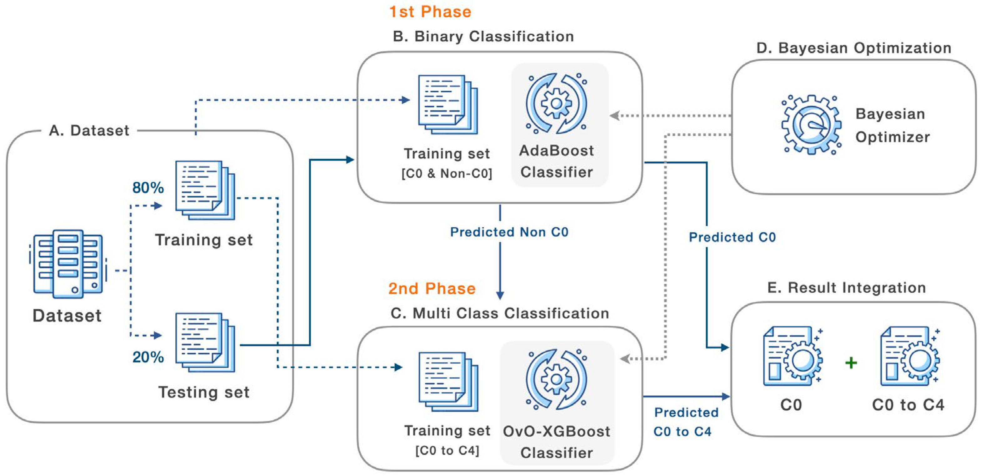
- The two-phase architecture of the grade prediction model is constructed using the ensemble approach. AdaBoost is utilized in the first phase as a binary classifier for categorizing class ‘c0’ and non-class ‘c0’. The remainder of the data will then be categorized using multi-class classification. In this phase, One-versus-One will collaborate with XGBoost to predict all of the grades. Due to the imbalanced dataset, this experiment’s data will not be over- or undersampled.
- This research presents new features that compute the distance between the data and the centroid of each grade class to determine how far the data points are from the center of each grade class.
- Adding many training features to a prediction model may diminish its performance. In this research, a silhouette coefficient-based feature selection is utilized for selecting only the data associated with the overlap of the grade clusters.
- The proposed architecture employs the Bayesian-based optimization algorithm to tune the ensemble methods’ hyperparameters.
2. Related Works
3. Methodology
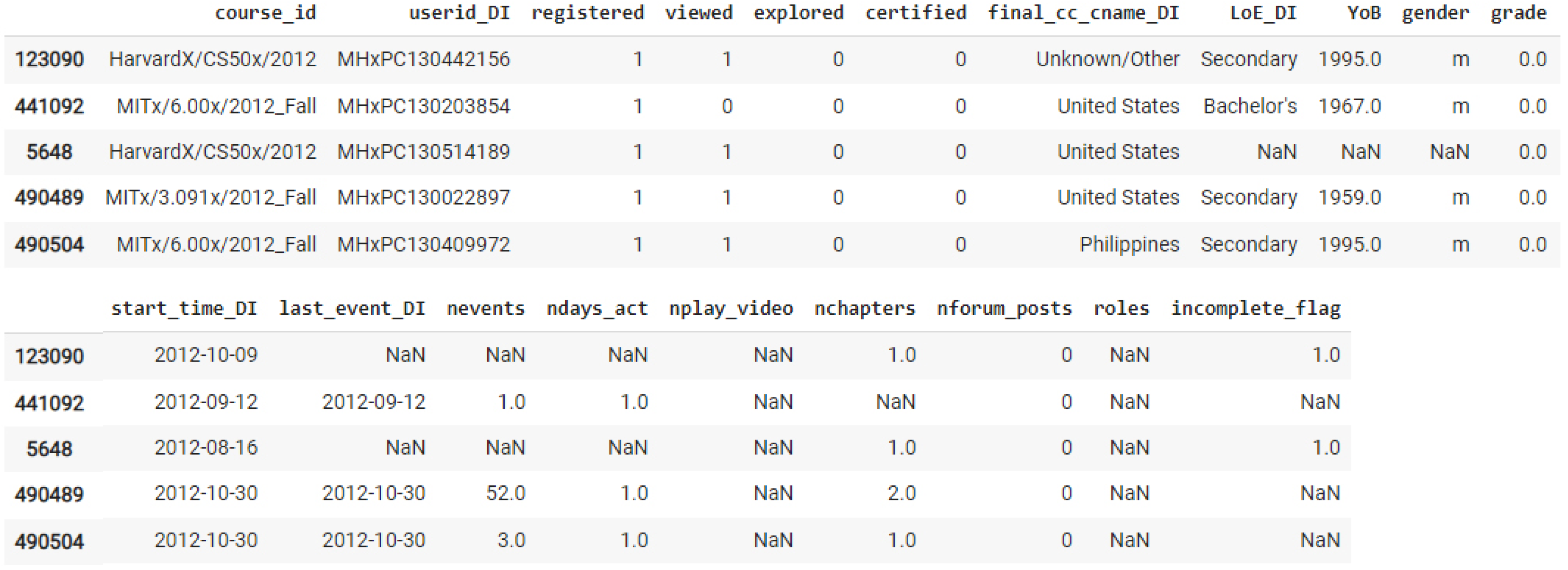
3.1. Dataset
3.1.1. HarvardX Person-Course Academic Year 2013 De-Identified Dataset (HMPC)
3.1.2. Canvas Network Person-Course (1/2014–9/2015) De-Identified Dataset (CNPC)
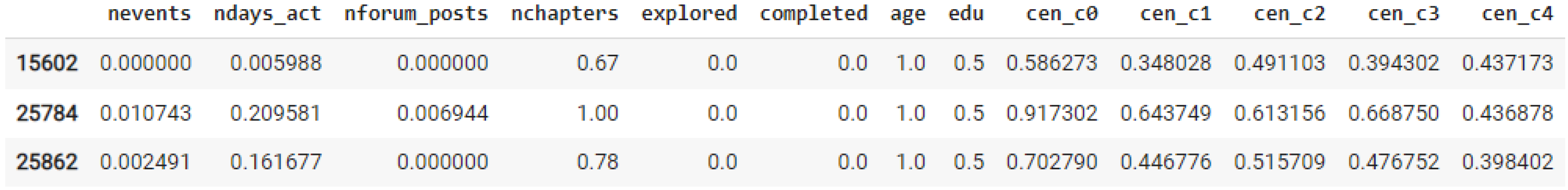
3.2. Data Pre-Processing
3.3. Centroid Distance Features and Selection Method
3.4. Machine Learning Architecture
- A.
- Dataset
- B.
- Binary Classification
- C.
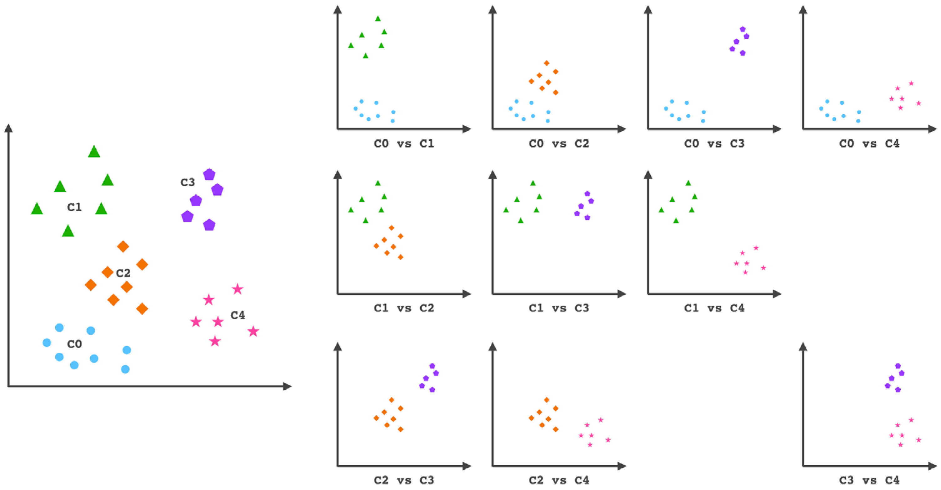
- Multi-Class Classification
- D.
- Bayesian Optimization
- E.
- Results Integration
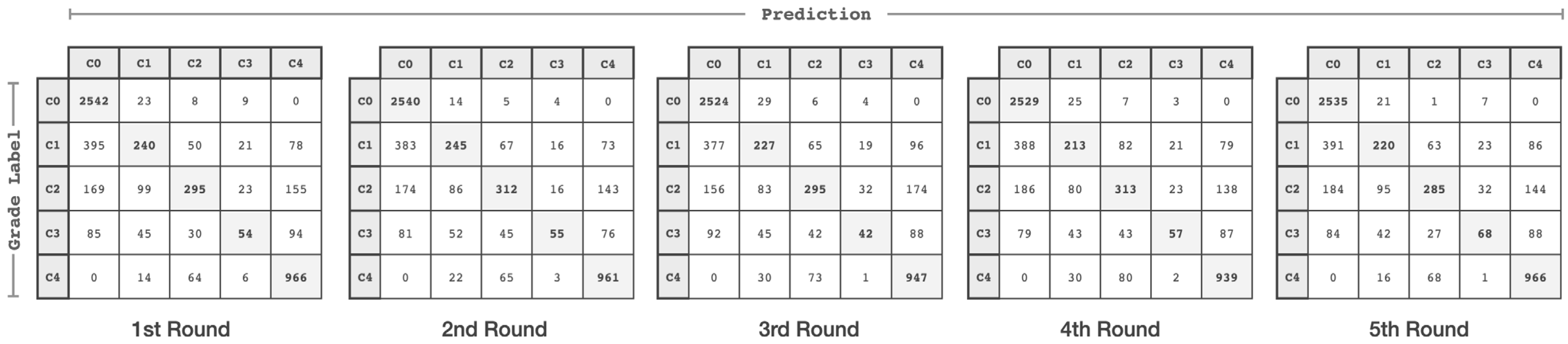
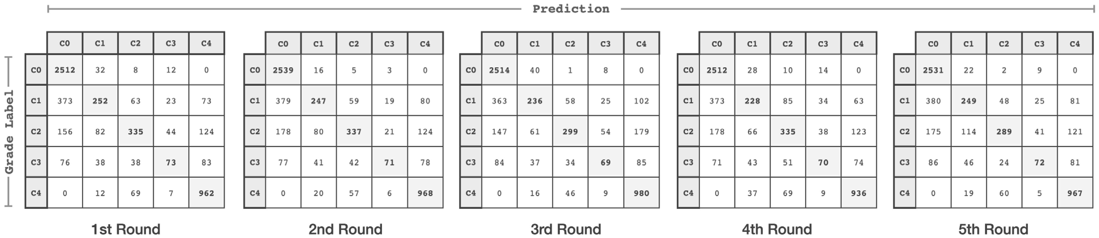
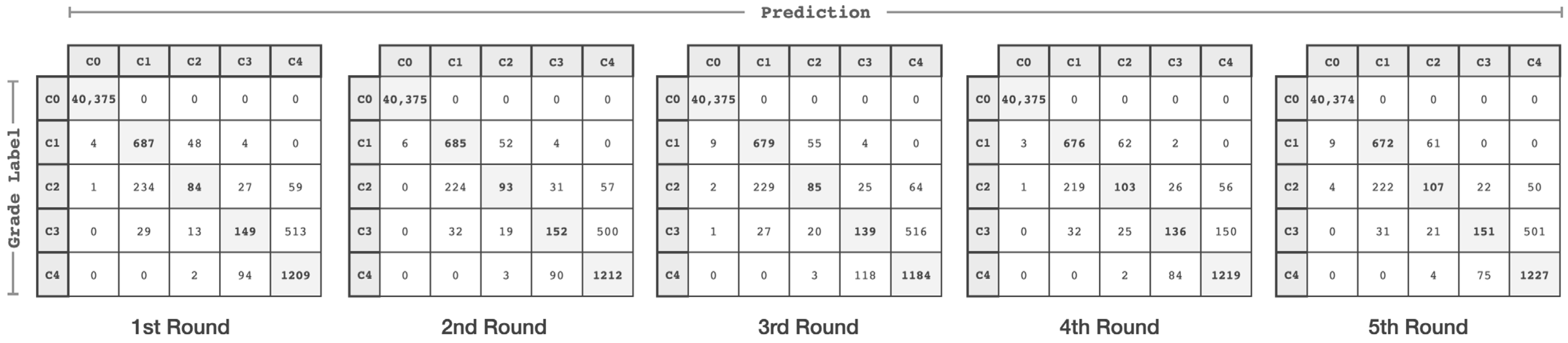
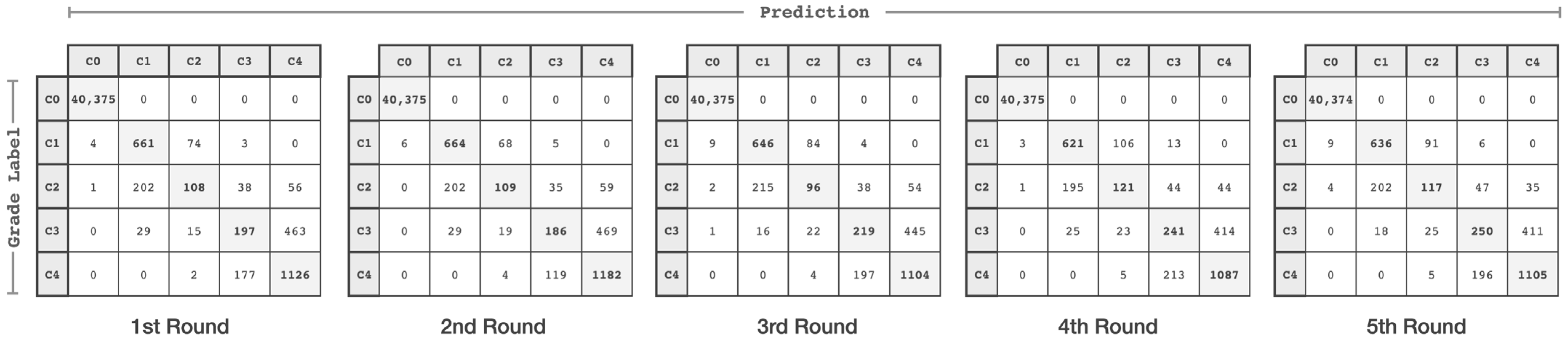
4. Performance Evaluation
5. Conclusions
Author Contributions
Funding
Institutional Review Board Statement
Informed Consent Statement
Data Availability Statement
Conflicts of Interest
References
- Pursel, B.K.; Zhang, L.; Jablokow, K.W.; Choi, G.W.; Velegol, D. Understanding MOOC students: Motivations and behaviours indicative of MOOC completion. J. Comput. Assist. Learn. 2016, 32, 202–217. [Google Scholar] [CrossRef]
- Pailai, J.; Wunnasri, W. Learning Behavior Visualization of an Online Lecture Support. ICIC Express Lett. Part B Appl. 2022, 13, 1155–1164. [Google Scholar]
- Abe, K.; Tanaka, T.; Matsumoto, K. Lecture support system using digital textbook for filling in blanks to visualize student learning behavior. Int. J. Educ. Learn. Syst. 2018, 3, 138–144. [Google Scholar]
- Kuosa, K.; Distante, D.; Tervakari, A.; Cerulo, L.; Fernandez, A.; Koro, J.; Kailanto, M. Interactive visualization tools to improve learning and teaching in online learning environments. Int. J. Distance Educ. Technol. 2016, 14, 21. [Google Scholar] [CrossRef]
- Hogo, M.A. Evaluation of e-learning systems based on fuzzy clustering models and statistical tools. Expert Syst. Appl. 2010, 37, 6891–6903. [Google Scholar] [CrossRef]
- Sakboonyarat, S.; Tantatsanawong, P. Massive open online courses (MOOCs) recommendation modeling using deep learning. In Proceedings of the 23rd International Computer Science and Engineering Conference, Phuket, Thailand, 30 October–1 November 2019. [Google Scholar]
- Albreiki, B.; Zaki, N.; Alashwal, H. A systematic literature review of student’performance prediction using machine learning techniques. Educ. Sci. 2021, 11, 552. [Google Scholar] [CrossRef]
- Kang, T.; Wei, Z.; Huang, J.; Yao, Z. MOOC student success prediction using knowledge distillation. In Proceedings of the Computer Information and Big Data Applications, Guiyang, China, 17–19 April 2020. [Google Scholar]
- Bujang, S.D.A.; Selamat, A.; Krejcar, O.; Mohamed, F.; Cheng, L.K.; Chiu, P.C.; Fujita, H. Imbalanced Classification Methods for Student Grade Prediction: A Systematic Literature Review. IEEE Access 2022, 11, 1970–1989. [Google Scholar]
- Douzas, G.; Bacao, F.; Fonseca, J.; Khudinyan, M. Imbalanced learning in land cover classification: Improving minority classes’ prediction accuracy using the geometric SMOTE algorithm. Remote Sens. 2019, 11, 3040. [Google Scholar] [CrossRef] [Green Version]
- Liang, X.W.; Jiang, A.P.; Li, T.; Xue, Y.Y.; Wang, G.T. LR-SMOTE—An improved unbalanced data set oversampling based on K-means and SVM. Knowl. -Based Syst. 2020, 196, 105845. [Google Scholar] [CrossRef]
- Mueller, M.; Weber, G. Machine Learning Regression Analysis of EDX 2012-13 Data for Identify The Auditors Use Case. Int. J. Integr. Technol. Educ. 2017, 6, 14. [Google Scholar] [CrossRef]
- Kuo, J.Y.; Chung, H.T.; Wang, P.F.; Baiying, L.E. Building Student Course Performance Prediction Model Based on Deep Learning. J. Inf. Sci. Eng. 2021, 37, 243–257. [Google Scholar]
- Xing, W.; Du, D. Dropout prediction in MOOCs: Using deep learning for personalized intervention. J. Educ. Comput. Res. 2019, 57, 547–570. [Google Scholar] [CrossRef]
- Ashraf, M.; Zaman, M.; Ahmed, M. An intelligent prediction system for educational data mining based on ensemble and filtering approaches. Procedia Comput. Sci. 2020, 167, 1471–1483. [Google Scholar] [CrossRef]
- Ayienda, R.; Rimiru, R.; Cheruiyot, W. Predicting Students Academic Performance using a Hybrid of Machine Learning Algorithms. In Proceedings of the 2021 IEEE AFRICON, Arusha, Tanzania, 13–15 September 2021. [Google Scholar]
- Yang, Y.; Fu, P.; Yang, X.; Hong, H.; Zhou, D. MOOC learner’s final grade prediction based on an improved random forests method. Comput. Mater. Contin. 2020, 65, 2413–2423. [Google Scholar] [CrossRef]
- Yang, Y.; Zhou, D.; Yang, X. A multi-feature weighting based K-means algorithm for MOOC learner classification. Comput. Mater. Contin. 2019, 59, 625–633. [Google Scholar] [CrossRef]
- Deepika, K.; Sathyanarayana, N. Hybrid model for improving student academic performance. Int. J. Adv. Res. Eng. Technol. 2020, 11, 768–779. [Google Scholar]
- Canvas Network Person-Course (1/2014–9/2015) De-Identified Open Dataset. Available online: https://doi.org/10.7910/DVN/1XORAL (accessed on 23 December 2022). [CrossRef]
- HarvardX Person-Course Academic Year 2013 De-Identified Dataset, Version 3.0. Available online: https://doi.org/10.7910/DVN/26147 (accessed on 23 December 2022). [CrossRef]
- Musil, C.M.; Warner, C.B.; Yobas, P.K.; Jones, S.L. A comparison of imputation techniques for handling missing data. West. J. Nurs. Res. 2002, 24, 815–829. [Google Scholar] [CrossRef]
- Sainis, N.; Srivastava, D.; Singh, R. Feature classification and outlier detection to increased accuracy in intrusion detection system. Int. J. Appl. Eng. Res. 2018, 13, 7249–7255. [Google Scholar]
- Yuan, C.; Yang, H. Research on K-value selection method of K-means clustering algorithm. J 2019, 2, 16. [Google Scholar] [CrossRef] [Green Version]
- Han, J.; Pei, J.; Tong, H. Data mining: Concepts and Techniques, 3rd ed.; Morgan Kaufmann: Burlington, MA, USA, 2012; pp. 489–490. [Google Scholar]
- Sun, Y.; Li, Z.; Li, X.; Zhang, J. Classifier selection and ensemble model for multi-class imbalance learning in education grants prediction. Appl. Artif. Intell. 2021, 35, 290–303. [Google Scholar] [CrossRef]
- Mienye, I.D.; Sun, Y. A Survey of Ensemble Learning: Concepts, Algorithms, Applications, and Prospects. IEEE Access 2022, 10, 99129–99149. [Google Scholar] [CrossRef]
- Yan, Z.; Chen, H.; Dong, X.; Zhou, K.; Xu, Z. Research on prediction of multi-class theft crimes by an optimized decomposition and fusion method based on XGBoost. Expert Syst. Appl. 2022, 207, 117943. [Google Scholar] [CrossRef]
- Sun, J.; Fujita, H.; Zheng, Y.; Ai, W. Multi-class financial distress prediction based on support vector machines integrated with the decomposition and fusion methods. Inf. Sci. 2021, 559, 153–170. [Google Scholar] [CrossRef]
- Song, Y.; Zhang, J.; Yan, H.; Li, Q. Multi-class imbalanced learning with one-versus-one decomposition: An empirical study. In Proceedings of the Cloud Computing and Security, Haikou, China, 8–10 June 2018. [Google Scholar]
- Le, T.T.H.; Oktian, Y.E.; Kim, H. XGBoost for imbalanced multiclass classification-based industrial internet of things intrusion detection systems. Sustainability 2022, 14, 8707. [Google Scholar] [CrossRef]
- Mardiansyah, H.; Sembiring, R.W.; Efendi, S. Handling problems of credit data for imbalanced classes using SMOTEXGBoost. J. Phys. Conf. Ser. 2021, 1830, 012011. [Google Scholar] [CrossRef]
- Snoek, J.; Larochelle, H.; Adams, R.P. Practical bayesian optimization of machine learning algorithms. Adv. Neural Inf. Process. Syst. 2012, 25, 9. [Google Scholar] [CrossRef]
- Mandl, T.; Modha, S.; Majumder, P.; Patel, D.; Dave, M.; Mandlia, C.; Patel, A. Overview of the hasoc track at fire 2019: Hate speech and offensive content identification in indo-european languages. In Proceedings of the 11th Forum for Information Retrieval Evaluation, Kolkata, India, 12–15 December 2019. [Google Scholar]
- Wawer, A.; Nielek, R.; Wierzbicki, A. Predicting webpage credibility using linguistic features. In Proceedings of the 23rd International Conference on World Wide Web, Seoul, Republic of Korea, 7 April 2014. [Google Scholar]


| HMPC | CNPC | After Pre-Processing | |
|---|---|---|---|
| Attribute | Attribute | Attribute | Example of Value |
| course_id | course_id_DI | - | - |
| userid_DI | userid_DI | - | - |
| registered | registered | - | - |
| viewed | viewed | - | - |
| explored | explored | explored | 1 |
| certified | completed_% | completed | 1 |
| - | course_reqs | - | - |
| grade | grade | grade | 0.75 |
| - | grade_reqs | - | - |
| - | primary_reason | - | - |
| final_cc_cname_DI | final_cc_cname_DI | - | - |
| - | primary_reason | - | - |
| - | learner_type | - | - |
| - | expected_hours_week | - | - |
| LoE | LoE | edu | “Bachelor’s” |
| YoB | age_DI | age | “{19–34}” |
| gender | gender | - | - |
| start_time_DI | start_time_DI | - | - |
| - | course_start | - | - |
| - | course_end | - | - |
| last_event_DI | last_event_DI | - | - |
| nevents | nevents | nevents | 502 |
| ndays_act | ndays_act | ndays_act | 16 |
| nchapters | nchapters | nchapters | 52 |
| nforum_posts | nforum_posts | nforum_posts | 8 |
| nplay_video | - | - | - |
| - | course_length | - | - |
| roles | - | - | - |
| inconsistent_flag | - | - | - |
| Class | HMPC | CNPC |
|---|---|---|
| C0 | 201,874 | 12,818 |
| C1 | 3714 | 3918 |
| C2 | 2025 | 3701 |
| C3 | 3517 | 1544 |
| C4 | 6526 | 5254 |
| Total | 217,656 | 27,235 |
| Silhouette Score between Each Class in the Dataset | HMPC | CNPC |
|---|---|---|
| C0 and C1 | 0.3299 | 0.1607 |
| C0 and C2 | 0.4772 | 0.3124 |
| C0 and C3 | 0.5884 | 0.2302 |
| C0 and C4 | 0.5948 | 0.3527 |
| C1 and C2 | 0.0676 | 0.0624 |
| C1 and C3 | 0.3482 | 0.0261 |
| C1 and C4 | 0.4290 | 0.1247 |
| C2 and C3 | 0.2263 | 0.0324 |
| C2 and C4 | 0.3281 | 0.0703 |
| C3 and C4 | 0.0325 | 0.1509 |
| Class | HMPC | CNPC |
|---|---|---|
| C0 | 201,874 | 12,818 |
| Non-C0 | 15,782 | 14,417 |
| Method | HMPC | CNPC | ||||
|---|---|---|---|---|---|---|
| Weighted Precision | Weighted Recall | Weighted Average F1 | Weighted Precision | Weighted Recall | Weighted Average F1 | |
| RF | 0.9715 | 0.9734 | 0.9720 | 0.6975 | 0.7274 | 0.7067 |
| RF + Selected distance feature | 0.9715 | 0.9734 | 0.9721 | 0.7040 | 0.7328 | 0.7127 |
| IRF [17] (without SMOTE) | 0.9720 | 0.9747 | 0.9721 | 0.6985 | 0.7272 | 0.7074 |
| RF Regression [12] | 0.9717 | 0.9747 | 0.9708 | 0.6893 | 0.6747 | 0.6779 |
| Deep Learning [13] | 0.9703 | 0.9705 | 0.9677 | 0.6649 | 0.7018 | 0.6712 |
| Proposed model | 0.9741 | 0.9764 | 0.9727 | 0.7149 | 0.7476 | 0.7110 |
| Proposed model + Selected distance features | 0.9732 | 0.9753 | 0.9734 | 0.7162 | 0.7486 | 0.7125 |
| Proposed model + Selected distance features + Bayesian Optimization | 0.9735 | 0.9756 | 0.9735 | 0.7270 | 0.7558 | 0.7236 |
| Machine Learning | HMPC | CNPC |
|---|---|---|
| AdaBoost | n_estimators = 10 learning_rate = 0.1 | n_estimators = 500 learning_rate = 1.0 |
| OvO + XGBoost | gamma = 10 max_depth = 40 min_child_weight = 1 n_estimators = 10 num_boost_round = 100 reg_alpha = 0.1 reg_lambda = 0.0 | gamma = 10 max_depth = 40 min_child_weight = 1 n_estimators = 100 num_boost_round = 1000 reg_alpha = 0.0 reg_lambda = 0.0 |
Disclaimer/Publisher’s Note: The statements, opinions and data contained in all publications are solely those of the individual author(s) and contributor(s) and not of MDPI and/or the editor(s). MDPI and/or the editor(s) disclaim responsibility for any injury to people or property resulting from any ideas, methods, instructions or products referred to in the content. |
© 2023 by the authors. Licensee MDPI, Basel, Switzerland. This article is an open access article distributed under the terms and conditions of the Creative Commons Attribution (CC BY) license (https://creativecommons.org/licenses/by/4.0/).
Share and Cite
Wunnasri, W.; Musikawan, P.; So-In, C. A Two-Phase Ensemble-Based Method for Predicting Learners’ Grade in MOOCs. Appl. Sci. 2023, 13, 1492. https://doi.org/10.3390/app13031492
Wunnasri W, Musikawan P, So-In C. A Two-Phase Ensemble-Based Method for Predicting Learners’ Grade in MOOCs. Applied Sciences. 2023; 13(3):1492. https://doi.org/10.3390/app13031492
Chicago/Turabian StyleWunnasri, Warunya, Pakarat Musikawan, and Chakchai So-In. 2023. "A Two-Phase Ensemble-Based Method for Predicting Learners’ Grade in MOOCs" Applied Sciences 13, no. 3: 1492. https://doi.org/10.3390/app13031492