Effect of Environmental Parameters on Structural Health Status Assessment Using OMA Techniques

Featured Application

The work presented in this paper is an investigation of the limitations of precision due to environmental disturbances (like thermal effects) in traditional algorithms based on operational modal analysis (OMA) that are used in dynamic structural health monitoring in civil and mechanical engineering.

Abstract

The data from a laboratory test on two aluminum rods are analyzed in this work. The rods are subjected to environmental excitation in an uncontrolled environment, attempting to replicate real operational conditions of structural health monitoring with external disturbances. Different damage levels are simulated on one of the two tension rods. Three of the most frequently used OMA methods are applied to evaluate the effects of the simulated damage on the dynamic behavior of the system. The complexity of the three applied OMA methods is gradually increased. The difference between the results from the different approaches is assessed. The aim of this work is to assess the performance of the proposed OMA methods, to understand their limits, and to assess the role of environmental disturbance parameters, such as temperature, in the evaluation of the health status of structures.

1. Introduction

Structural health monitoring (SHM) is the process of checking the condition of a structure through an automated monitoring system. SHM techniques started in aerospace and automotive fields, but due to their multidisciplinary nature and potential, in the last decades they are widely used and adapted for civil engineering.

In an SHM process, the data acquisition can be carried out periodically, or as is more common in recent years, continuously. In this second case, the volume of sampled data may be not negligible, and therefore advanced data management skills are needed [1,2].

The objectives of SHM can be divided into the following five levels [2,3]:

• Damage detection: giving a qualitative indication of the probable presence of damage in the monitored system.
• Damage localization: giving an information about the probable location of the damage in the monitored system.
• Damage classification: giving an information about the possible type of damage.
• Damage assessment: giving an estimate of the probable extent of damage.
• Damage prognosis: giving information on the structural safety, e.g., estimating the useful life of the structure after damage.

High-order levels generally require the information necessary to determine the lower order levels. The first two levels will be investigated in this work for the monitoring of the examined system.

The development of an SHM-based method generally depends on two key factors: the technology of the sensor used for monitoring, and the algorithm used for the interpretation of sampled signals. A structural monitoring system generally consists of several key components: sensors, data acquisition, data transmission, data processing, data storage, and structural health assessment [2]. Each of these phases plays a key role. The following work will examine the stages of data processing and health assessment.

Strategies for monitoring the health status of a structure can be categorized into two main groups that generally provide different types of information [2]: global monitoring and local monitoring. The most appropriate type of monitoring depends on the kind of structure. For example, a global approach should be chosen when access to specific parts of the structure is impossible [2]. For a global monitoring system, accelerometers are one of the most-used type of sensors. The measurement of acceleration data can be used to estimate the modal parameters of the system and damage can be investigated by evaluating their variation over time.

In this paper, a global approach was used. Two aluminum rods are monitored by means of a network of accelerometers. A series of simulated damages of different magnitudes were simulated in different positions of the rods by adding small masses. The modal parameters of the system were derived using different OMA techniques. The raw modal parameters were cleaned of environmental thermal effects to separate the effect of environmental disturbance parameters from the effect of the damage. The effectiveness of the applied OMA methods and the limits of the monitoring system were evaluated, studying the capacity for detecting the variation of the modal parameters due to applied damage without being blinded by the ambient disturbances.

OMA techniques have been studied for years and are well established nowadays. In recent years, many studies have been conducted on automatic OMA techniques that allow the automatic identification of modal parameters. These techniques are particularly suitable in continuous monitoring situations over long periods [4,5,6].

However, there has never been enough focus on the aspects that can influence the interpretation of dynamic identification results. In fact, the dynamic behavior of most types of structure is strongly influenced by the environmental conditions in which the structure operates. The influence of environmental conditions can mislead the assessment of the health status of the structure. Therefore, their influence on the modal parameters must be studied very carefully. The authors of this paper would like to highlight this last aspect.

2. Dynamic Monitoring

Dynamic monitoring of a structure is the process of assessing structural characteristics through the study of induced vibrations [1]. It is based on the hypothesis that a change in the mechanical characteristics of the structure due to damage or deterioration causes a more or less appreciable change in the structural dynamic behavior [1]. An extensive description and classification on modal analysis methods is given in [1] and [7]. Modal parameters, such as natural frequencies, mode shapes and their variants, and damping are commonly used in SHM. However, the use of natural frequencies alone as damage indices has some limitations; they are quite insensitive to local damage and the number of available frequencies is limited—generally less than 10 [8].

For multi-degree-of-freedom (MDOF) systems, the dynamic behavior can be described by a system of differential equations in the time domain, shown in expression (1).

$$\left[M\right]\left\{\ddot{y}\left(t\right)\right\}+\left[C\right]\left\{\dot{y}\left(t\right)\right\}+\left[K\right]\left\{y\left(t\right)\right\}=\left\{f\left(t\right)\right\}$$

(1)

where: $\left\{\ddot{y}\left(t\right)\right\}$, $\left\{\dot{y}\left(t\right)\right\}$ and $\left\{y\left(t\right)\right\}$ are the vectors of acceleration, velocity and displacement, respectively; $\left[M\right]$, $\left[C\right]$ and $\left[K\right]$ are the mass, damping and stiffness matrices, respectively; and $\left\{f\left(t\right)\right\}$ is the forcing vector. Expression (1) is valid for a linear, invariant ($\left[M\right]$, $\left[C\right]$ and $\left[K\right]$ are constant), observable system with viscous damping. It describes the dynamic behavior of a system with N degrees of freedom. The equation of motion, which is coupled in this formulation, can be decoupled under the assumption of viscous proportional damping using the principle of orthogonality between the modes of vibration and solving an eigenvalue problem. This leads to a system of algebraic equations and the modal model [1,2,7,9,10].

The dynamic model at the basis of the most used OMA methods, which is proposed in the following, is represented by the model in phase space. This is obtained through a series of mathematical manipulations of the spatial model shown in (1) [1]. In the phase-space model, the dynamic behavior of the structure is described through three fundamental matrices: the state matrix [A], the controllability matrix [C] and the observability matrix [O].

A fundamental role for the application of methods based on operational modal analysis is played by the theories of signal analysis [1,2]. The roles played by statistical operators, especially second-order operators (correlation functions), and by transformations from time to frequency domain, i.e., the Fourier transform, are fundamental.

3. Methodology

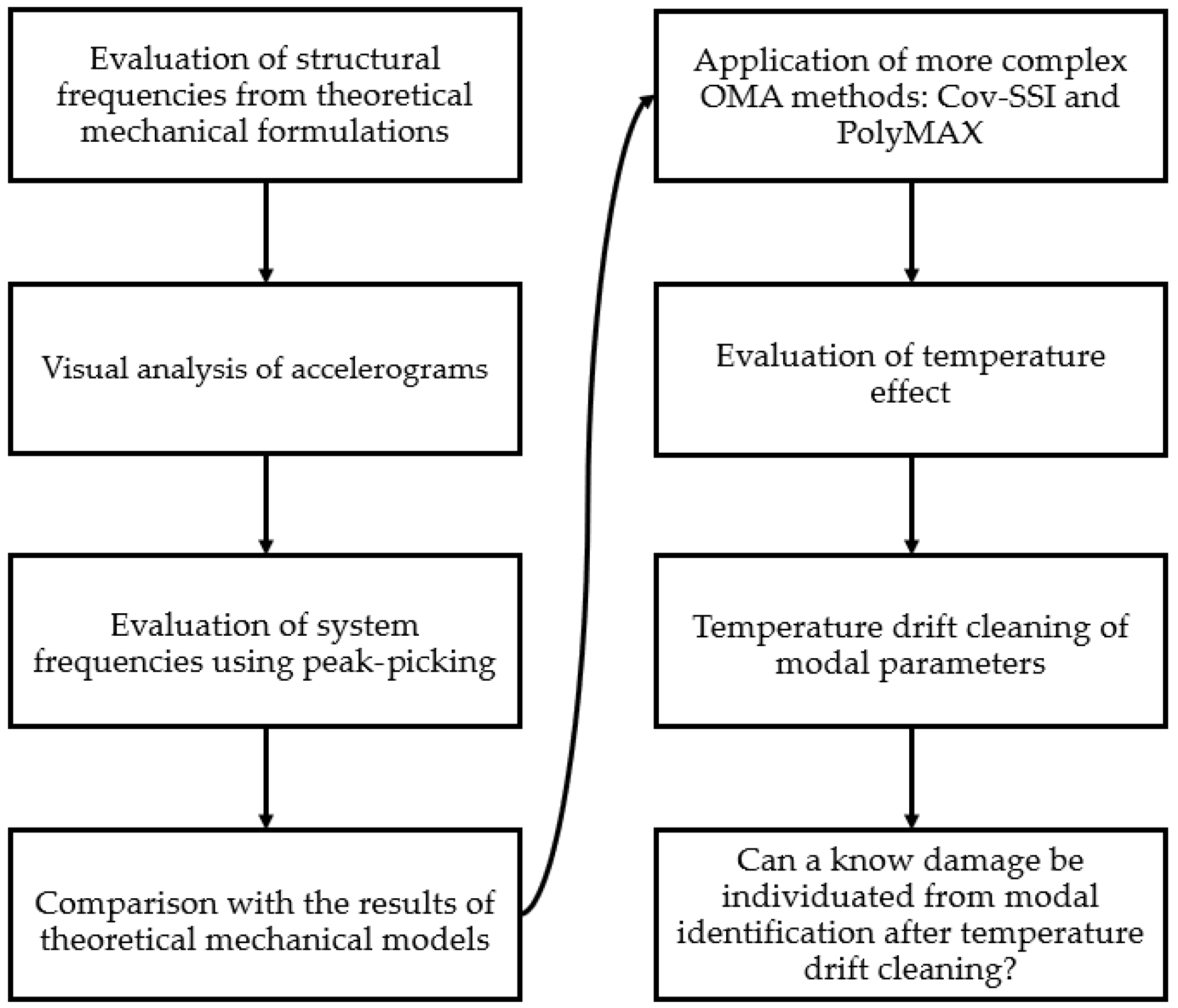
In this section, the authors describe the methodology followed in the study. In the first step, the accelerometer data are observed, and a simple visual assessment is made to see if there is any macroscopic anomaly. If no anomaly is found visually, the accelerometer data are analyzed using the peak-picking method; the simplest and least computationally demanding OMA method.

The frequencies obtained by peak-picking are then compared with the theoretical results obtained from mechanical formulations of vibrating rods and ropes.

After this first phase, two more complex OMA methods with higher computational burdens are applied: Cov-SSI and PolyMAX. The frequencies of the first three vibration modes are calculated.

These frequencies show a trend over time that is correlated with the ambient temperature trend. The correlation with temperature is cleaned to the best possible standard and the reliability of the cleaned frequencies is assessed, attempting to find known damages introduced in the rods.

Figure 1 shows the flow-chart of the study.

4. Applied OMA Methods

Three of the most used OMA methods are used in this paper. The results obtained from their application are compared to understand which method is the most effective in providing early warning of damage in the examined structure in a noisy environment. A parametric method in the time domain, Cov-SSI [1,7,11], and two methods in the frequency domain; a non-parametric method, peak-picking [1]; and a parametric method, poly-reference least-squares complex-frequency method (PolyMAX) [1,12,13], are examined.

4.1. Peak-Picking

Peak-picking is the non-parametric method in the frequency domain that requires the lowest computational burden. It is based on the evaluation of the power spectral density [14,15,16]. The name of the method derives from the fact that the proper modes of the structure are identified by looking for peaks in the power spectral density (PSD) graph [1]. The PSD is estimated by the Welch method [17] as follows.

$${\widehat{G}}_{xx}\left(f\right)=\frac{2}{nN{t}_s}{\displaystyle \sum }_{i=1}^n{\left|X_i\left(f\right)\right|}^2$$

(2)

where ${\widehat{G}}_{xx}\left(f\right)$ is the one-sided auto-spectral density function; $n$ is the number of contiguous segments into which the signal is split; $N{t}_s$ is the length of each segment into which the signal has been divided; and ${\left|X_i\left(f\right)\right|}^2$ is the FFT of the segment.

A few preventive operations, such as the application of appropriate windows to the raw signal to avoid the leakage phenomenon, need to be performed on the raw signal before applying Welch’s method [1,7,9,14,15,18].

The peak-picking method assumes that in proximity to the structure’s resonance, close to the peak, the structure behaves like a one-degree-of-freedom system (1DOF), as only one mode is dominant, and the contribution of the other modes can be neglected.

This method has the advantage of providing an acceptable approximation of the modal parameters of the system quickly and easily if the modes are well separated, but it shows low accuracy and an inability to identify modes that are very close to each other, or cases of high damping [1]. It is especially useful for a first check on the sampled data and for a first estimation of the modal parameters of the system.

In the present work, the peak-picking method is applied on a single sensor output. A MDOF approach with frequency-domain decomposition (FDD), based on the SVD of the 3D PSD matrix, is not performed.

4.2. Covariance-Driven Stochastic Subspace Identification (Cov-SSI)

Cov-SSI is one of the most effective and widely used methods in civil engineering. It is a parametric method in the time domain. It approaches the problem of stochastic realization, identifying a stochastic model from output-only data [1,7,11,19]. A complete and exhaustive mathematical treatment of the method can be found in [1].

The system under evaluation should be observable and controllable [20]; for a system of order N, its observability and controllability matrices must have rank N. In practice, the order of the system is unknown, and its accurate determination is very complex due to the uncertainty and the noise that accompanies the sampling. For this reason, a conservative approach will overestimate the system order. This will cause the appearance of non-physical modes that must be separated from the physical modes by specific methods represented by the stabilization diagrams [1,7].

Only the poles that exhibit stability between the different orders of the model represent physical modes. The most used stability criteria, as reported in [1], are generally the following:

$$\frac{\left|f\left(n\right)-f\left(n+1\right)\right|}{f\left(n\right)}<0.01$$

(3)

$$\frac{\left|\zeta \left(n\right)-\zeta \left(n+1\right)\right|}{\zeta \left(n\right)}<0.05$$

(4)

where $f\left(n\right)$ is the natural frequency of the order $n$ model; $\zeta \left(n\right)$ is the damping of the order $n$ model; $f\left(n+1\right)$ is the natural frequency of the order $n+1$ model; and $\zeta \left(n+1\right)$ is the damping of the order $n+1$ model.

4.3. Poly-Reference Least-Squares Complex Method (PolyMAX)

PolyMAX is a parametric frequency domain model of operational modal analysis [1,7,12,13]. It is a method based on least-squares complex-frequency (LSCF) -type estimators [1]. Its main advantage is the possibility of obtaining very clear stabilization diagrams [1,12]. As a parametric method, it has a high complexity and high computational effort. It is based on the right fraction of the FRF (frequency response function) matrix.

$$\left[H\left(\omega \right)\right]=\left[B_R\left(\omega \right)\right]{\left[A_R\left(\omega \right)\right]}^{-1}$$

(5)

where $\left[H\left(\omega \right)\right]$ is the FRF matrix; $\left[B_R\left(\omega \right)\right]$ is the numerator polynomial matrix and ${\left[A_R\left(\omega \right)\right]}^{-1}$ is the denominator polynomial matrices.

The FRF matrix relates the inputs exciting the system to the system’s response. In the case of operational modal analysis, the system inputs are unknown, so the analogy between PSD matrix and FRF matrix is used, assuming that the input is wide-band noise. The common-denominator model (also known as the scalar matrix-fraction model) of the FRF represents a special case of the right fraction of a matrix, where the numerator is a polynomial matrix and the denominator is a polynomial characterized by scalar coefficients.

$$\left[H\left(\omega \right)\right]=\frac{\left[B\left(\omega \right)\right]}{\left[A\left(\omega \right)\right]}=\frac{{\sum }_{j=0}^n\left[{\beta }_j\left(\omega \right)\right]{\Omega }^j\left(\omega \right)}{{\sum }_{j=0}^n{\alpha }_j{\Omega }^j\left(\omega \right)}$$

(6)

where ${\Omega }^j\left(\omega \right)$ is the polynomial basis function, which is used to describe a frequency-domain model that is derived from a discrete-time model; $n$ is the model order; ${\beta }_j\left(\omega \right)$ are the numerator matrix polynomial coefficients; and ${\alpha }_j$ are denominator matrix polynomial coefficients.

The least squares complex frequency (LSCF) method is based on the common denominator model shown in (6). The PolyMAX method is an extension of the LSCF motivated by some limitations arising from the application of the common denominator model in the LSCF method. The most important limit of LSCF is the difficulty in identifying very close modes [1].

By deriving the modal parameters for different model orders, the stabilization diagram can be constructed. As in the Cov-SSI algorithm, the pole alignment indicates the modal parameters of the system under examination.

For the complete and exhaustive mathematical treatment of the method, reference can be found in [1,13].

5. Description of the Experimental Set-Up

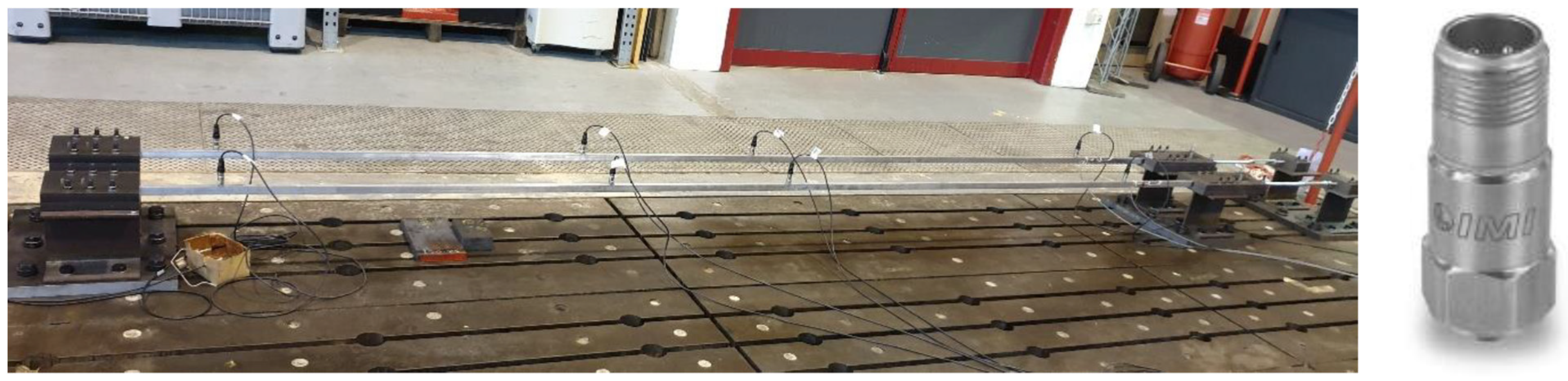
Continuous monitoring is performed on two aluminum tensioned rods with the same geometric characteristics and subject to environmental excitation. The experimental set-up is shown in Figure 2.

The geometrical characteristics of the rods are given below:

• Material: aluminum 6000 series.

  o

  Density: 2700 kg/m³

  o

  Young modulus: 69 GPa

• Beam cross section: rectangular, with base $b=15 \mathrm{mm}$ and depth $h=25 \mathrm{mm}$.
• Clear span between fixed ends $L=4000 \mathrm{mm}$.
• Nominal tensile force in the beams T= 8 kN (axial force at installation). The axial force is then variable because of environmental thermal cycles.

Each of the two rods is equipped with the following instrumentation:

• 4 single axis piezo accelerometers, placed in vertical direction, model 603C01 produced by PCB PIEZOTRONICS [21]. They are industrial accelerometers with a sensitivity of 0.1 V/g, a full scale $\pm 50 \mathrm{g}$, frequency range 0.5$÷$10,000 Hz.
• Strain gages arranged in a full-bridge configuration to measure tension. The conditioning unit is a National Instrument board NI 9236 and the system has been pre-calibrated against a certified load cell.

A thermocouple measuring ambient temperature during the test is also present and connected to a conditioning device with an analog output, so that temperature data can be acquired together with acceleration data. Only ambient air temperature is measured, not the temperatures of the aluminum rods.

Figure 2. Experimental setup and accelerometers used [22].

Figure 2. Experimental setup and accelerometers used [22].

All data are sampled thanks to a series of National Instruments NI 9234 boards, having a $\pm 5V$ full scale and a 24 bit ADC; data have been collected at a sampling frequency $f_s=512 \mathrm{Hz}$, considered enough to measure at least the first vibration modes of interest. A global acquisition time $T_{acquisition}$ of 600 s has been chosen.

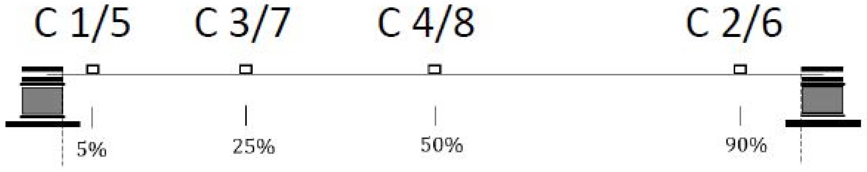
Figure 3 shows the position of the accelerometers on the rods; they are named with the letter C followed by a number, indicating the column of the matrix in which the data for that accelerometer are collected. For beam 1, the sensors are C1, C2, C3 and C4 and the accelerometer data are collected in column 1, 2, 3 and 4 of the acquisition matrix. For Beam 2, the sensors are C5, C6, C7 and C8 and the accelerometer data are collected in columns 5, 6, 7 and 8 of the acquisition matrix.

6. Mechanical Model

The experimental setup was mechanically modelled to obtain a theoretical prediction of the natural frequencies of the rods for a comparison with the identified frequencies.

The exact constraint conditions of the rods are not known in detail, as the level of restraint provided by the clamps and the strong floor (see Figure 2) is difficult to estimate. The aluminum rods are clamped to the test floor using the mechanical restraints visible in Figure 2. The bending stiffness of these restraint is not zero and not infinite; therefore, the rod has an unknown level of rotation restraint at the ends.

Several different mechanical approximations of the rods were studied: tensed rope; simply supported beam with and without axial force; and fully restrained beam with and without axial force. Some structural schemes that may seem quite different from the real schemes are taken into consideration to fully understand the effect of each mechanical parameter on the structural behavior.

6.1. Tensed Rope

As a first approximation, the rod can be considered as a tensed rope, neglecting its bending inertia due to the great slenderness of the profile. The frequencies can therefore be obtained in the following way [23]:

$$f_n=n\frac{1}{2L}\sqrt{\frac{T}{m}}$$

(7)

where T represents the tensile force in the beam, L the span, and m the mass per unit length.

These frequencies should be lower than the real frequencies because the bending stiffness is neglected.

6.2. Simply Supported Beam without Axial Force

The natural frequencies of a simply supported beam without axial force are [24,25]:

$$f_n=\frac{1}{T_n} T_n=\frac{2\pi }{{\omega }_n}=\frac{2L^2}{\pi n^2}\sqrt{\frac{m}{EI}}$$

(8)

where: $T_n$ is the period of the n-th mode, L is the beam length, n is the mode number (n = 1, 2, 3, …), m is the mass per unit length (m = 1.0125 kg/m), E is the Young modulus of alluminuim, and I is the inertia of the cross section related to vertical bending ($I=1.953·{10}^{-8} {\mathrm{m}}^4$).

These frequencies should also be lower than the real frequencies because the bending stiffness is taken into account, but the stiffening effect of the axial load is neglected.

6.3. Simply Supported Beam with Axial Force

The natural frequencies of a simply supported beam subjected to axial force can be calculated according to [24,25]:

$$f_n=\frac{n^2\pi }{2L^2}\sqrt{1+\frac{T{L}^2}{EI{n}^2{\pi }^2}}\sqrt{\frac{EI}{m}}$$

(9)

All the parameters are already explained in Section 6.1 and Section 6.2

These frequencies should again be lower than the real frequencies because the bending stiffness of the clamps is not taken into account.

6.4. Fully Restrained Beam without Axial Force

The natural frequencies of a fully restrained beam without axial force can be calculated according to [24,25]:

$$\cos \left({\alpha }_{n}L\right)\cosh \left({\alpha }_{n}L\right)=1$$

(10)

The first five solutions are: ${\alpha }_{1}L=4.730, {\alpha }_{2}L=7.853, {\alpha }_{3}L=10.996, {\alpha }_{4}L=14.137,{\alpha }_{5}L=17.279$, where $\alpha =\sqrt[4]{\frac{m{\omega }^2}{EI}}$, and $\omega$ is the circular frequency.

6.5. Fully Restrained Beam with Axial Force

When a fully restrained beam is also subjected to axial force, the natural frequencies can be calculated according to [24,25] as follows.

$$f_{n,T\ne 0}=f_{n,T=0}{\left(1+\gamma \frac{T}{P_{cr}}+\frac{1}{\frac{1}{\alpha \gamma }\frac{P_{cr}}{T}+\frac{1}{\beta }}\right)}^{0.5}$$

(11)

where $\alpha ,\beta , e, \gamma$ are parameters depending on boundary conditions and on the considered mode (see

Table 1. Boundary conditions parameters for fully restrained beam.

Mode	α	β	γ
1	0.195	1.211	0.816
2	0.148	1.151	0.857
3	0.088	0.996	0.979
4	0.068	0.828	0.991
5	0.055	0.739	0.996

) and $P_{cr}$ is the critical axial load, evaluated using the inertia moment, I, of the cross section of the beam related to vertical bending:

$$P_{cr}=\frac{4{\pi }^{2}EI}{L^2}$$

(12)

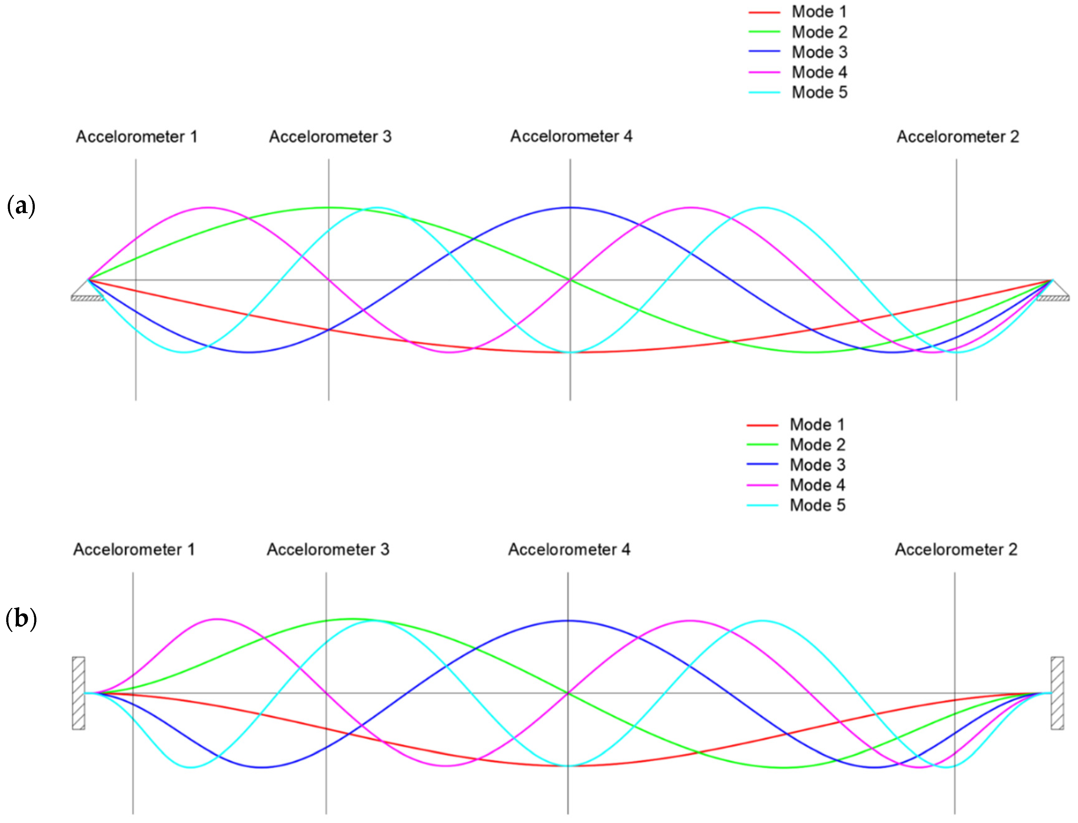
The natural frequencies obtained under the different hypotheses described in the previous paragraphs are presented in

Table 2. Comparison between natural frequencies calculated with different static schemes.

Mode	Frequency [Hz]
	1 Tens. Rope T ≠ 0	2 Simply Supp. T = 0	3 Simply Supp. T ≠ 0	4 Fully Restrained T = 0	5 Fully Restrained T ≠ 0
1	11.11	3.58	11.67	8.12	14.65
2	22.22	14.33	26.44	22.38	40.69
3	33.33	32.24	46.37	43.88	82.40
4	44.44	57.31	72.52	75.53	141.69
5	55.56	89.54	105.38	108.35	202.93

. The outputs of each mode refer to similar modal shapes. The modal shapes of the first 5 vibration modes are shown in Figure 4 for simply supported beam and fully restrained beam conditions.

If we compare the results of the tensed rope scheme with the simply supported scheme with axial force, it is possible to observe that for the low order modes (1 and 2) the rope-like behavior is common (11.1 ≅ 11.7 and 22.2 ≅ 26.4). On the contrary, when the modal order increases, the bending inertia starts playing a dominant role, increasing the natural frequencies (46.3 > 33.3, 72.5 > 44.4, etc.).

From the comparison of column 3 with column 5, it can be seen that the effect of the full restraint at the ends is smaller for the low order modes (+26% for Mode 1) than for high order Modes (+92% for mode 5).

The laboratory-tested rods should behave like tensed beams with an intermediate boundary condition between hinge and full restraint; therefore, the authors expected the rod specimens to have the first three natural frequencies within the limits listed below:

• $11.7\le f_1 \le 14.7 \mathrm{Hz}$ (lab $f_1\cong 14 \mathrm{Hz})$
• $26.4\le f_2 \le 40.7 \mathrm{Hz}$ (lab $f_2\cong 31 \mathrm{Hz})$
• $46.4\le f_3 \le 82.4 \mathrm{Hz}$ (lab $f_3\cong 53 \mathrm{Hz})$

The values effectively measured in the lab confirmed these design hypotheses.

7. Data Analysis with Applied OMA Methods

In this section, a portion of the sampled data is analyzed using the three OMA methods. The system’s own frequencies are chosen as the modal reference parameters to be studied.

The following datasets are analyzed:

• 72-h dataset: both rods in nominal condition. For both Beam 1 and Beam 2, this dataset is called: “Nominal Conditions”.
• 12-h dataset: Beam 1 with an additional mass in midspan equal to 1% of its nominal mass and Beam 2 in nominal condition. This dataset is called “Mass 1%” for Beam 1 and “Set 1” for Beam 2.
• 12-h dataset: Beam 1 with additional mass in midspan equal to 3% of the nominal mass of the beam and Beam 2 in nominal condition. A disturbance coming from a fatigue test carried out in the same lab affects this dataset. This dataset is called “Mass 3% a” for Beam 1 and “Set 3 a” for Beam 2.
• 12-h dataset: Beam 1 with additional mass in midspan equal to 3% of the nominal mass of the beam and Beam 2 in nominal condition. This dataset is called “Mass 3% b” for Beam 1 and “Set 3 b” for Beam 2.
• 12-h dataset: Beam 1 with additional mass at L/10 equal to 5% of the nominal mass and Beam 2 in nominal condition. This dataset is called “Mass 5%” for Beam 1 and “Set 5” for Beam 2.

In each of the twelve-hour datasets, a mass is fixed on Beam 1 to decrease the natural frequencies of the rod in order to simulate the effect of a reduction of cross-section without effectively damaging the rods. The presence of a mass generates an effect similar to the reduction of the cross section: the bigger the mass introduced, the more severe the virtual damage is. The magnitude of the added masses is very small compared with the mass of the beam; therefore, the effect of the simulated damage is small and difficult to investigate because of thermal actions and ambient noise. This choice is aimed to evaluate the sensitivity of the different OMA methods applied.

The data sets are discretized in intervals of constant length of 5 and 10 min, both granting an adequate spectral resolution. Five- and ten-minute intervals are chosen to evaluate the effect of the record length on the effectiveness of the adopted algorithms. All data analysis has been carried out in MatLab [26].

Cov-SSI and Poly-Reference Least Squares Complex Frequency Method imply a high computational burden; therefore, the only modal parameter chosen as an indicator of damage at this stage are the frequencies of the system vibrational modes. Obviously, this approach has limitations [8], but considering the simplicity of the structural system analyzed, it provides good results.

7.1. Application of the Peak-Picking Method

The PSDs are estimated using Welch’s method with a Hanning-type window with three different extensions: 1 min, 30 s and 15 s.

Two PSDs coming from two different sampling intervals for Beam 1 under nominal conditions (72-h dataset) are shown in Figure 5. Windows with a larger amplitude (i.e., 1 min) provide higher PSD frequency resolution. On the other hand, a smaller window width guarantees a higher number of averages, with a reduction in the signal–to–noise ratio. In this paper, fairly large windows were used in order to guarantee good frequency resolution to be able to investigate frequency variations arising from small damages.

By comparing the two diagrams shown in Figure 5, it is possible to notice a considerable variability in the amplitude of the peaks between the intervals due to different levels of environmental excitation during sampling. Furthermore, in some intervals, the peaks are confused with the PSD noise, as happens for the first peak; present in Figure 5a around 14Hz and not present in Figure 5b. In this paper, the amplitude of the peaks is not taken into consideration because the uncontrolled environmental conditions cause the peaks’ amplitudes to vary considerably. Only the position of the peaks is assessed. The signal–to–noise ratio is relatively low, as the two beams are only subjected to ambient excitation. Therefore, when there is very little environmental excitation, noise dominates, especially during the night when no human activity is present in the laboratory. In addition, the first frequency of the rods is about 14 Hz (because they are tensed) which is difficult to excite with ambient excitations. The second and third mode are therefore even more difficult to excite.

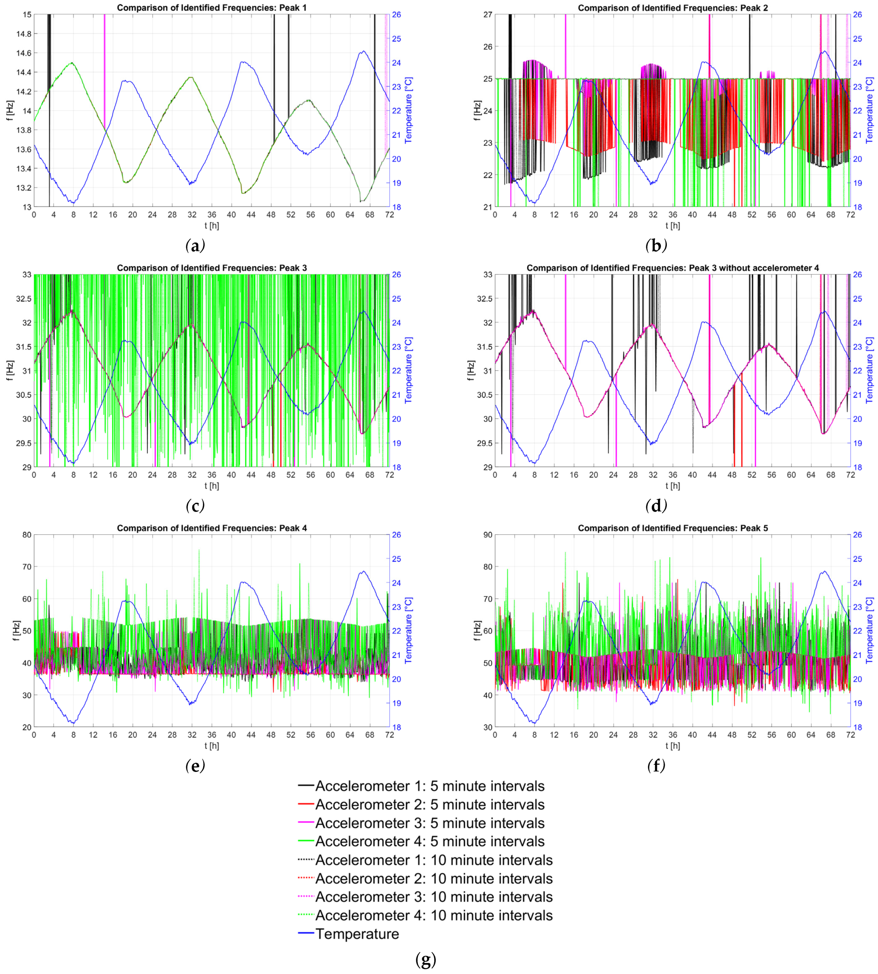
The peak-picking operation is performed by using the ‘findpeaks’ function of the MatLab package [26]. The results obtained for Beam 1 under nominal conditions (72-h data set) are shown in Figure 6.

Peak 1—Figure 6a—has a frequency between 14.5 and 13 Hz with an inverse correlation between the frequency and the environmental temperature. This range of frequencies (with an average of 13.8 Hz) lies between the natural frequencies calculated for the simply supported beam and the fully restrained beam in Section 6 (11.67 < 13.8 < 14.65).

Peak 2—Figure 6b—is around the frequency of 25 Hz. The lack of correlation with ambient temperature suggests that this peak represents a narrow band not controlled excitation, rather than a dynamic system behavior; this is an important warning about the verification of the presence of broad-band noise excitation to properly work with OMA. In addition, 25 Hz lies outside the range of natural frequencies calculated for Mode 2 in Section 6.

Peak 3—Figure 6c,d—has a frequency between 32.3 and 29.7 Hz, with inverse correlation between identified frequencies and ambient temperature. Moreover, Accelerometer 4, positioned in the middle of the beam, is ineffective as it is blinded by noise; therefore, Peak 3 can represent an even-order vibration mode of the beam. The natural frequencies calculated for Mode 2 for the simply supported beam and the fully restrained beam in Section 5 are well coupled with the results for this peak (22.4 < 31.0 < 40.7).

The frequencies of Peak 4 and Peak 5—Figure 6e and Figure 6f—can be found around 50 Hz, inversely correlated with temperature; however, the outputs are considerably disturbed. This is due to the fact that high-order modes are difficult to excite; in PSD they are confused with the noise of the transform.

It should be noted that the vertical lines in Figure 6 represent outliers, i.e., frequencies that cannot be identified. The presence of these outliers increases with increase in the mode order being considered.

In conclusion, the peak-picking method proves efficient for the low-order modes, which are those most easily excited and therefore more easily detected. For the higher order modes, which are harder to excite, the signal–to–noise ratio becomes unfavorable; the signal starts to be buried in the PSD noise and the output can hardly be used for damage detection.

Nevertheless, peak-picking can be useful in a preliminary analysis to understand the overall structural behavior.

7.2. Application of the Cov-SSI Method and the Poly-Reference Least Squares Complex Frequency Method

Two of the most widely used methods of operational modal analysis are presented in this paragraph: Cov-SSI and PolyMAX.

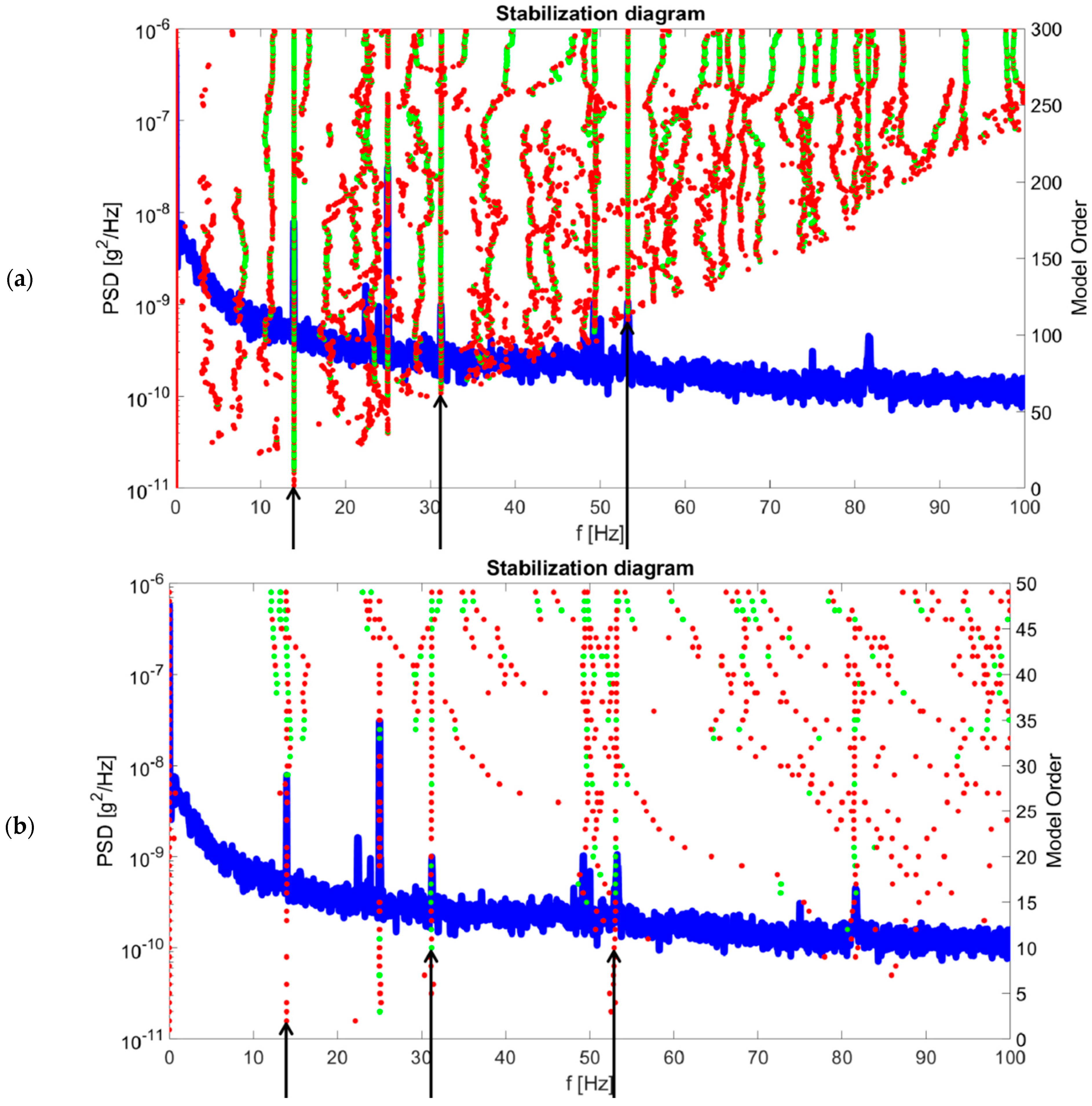
Figure 7 compares two stabilization diagrams obtained from the application of the two methods. They are both obtained for a 5-min record extracted at the 36th hour of sampling for Beam 1 under nominal conditions (72-h dataset).

Red dots indicate unstable poles, i.e., where one of the two conditions expressed in Equations (3) and (4) is not fulfilled. The green points indicate stable poles, where both conditions expressed in Equations (3) and (4) are fulfilled. Where the stable poles (green dots) align vertically, a structural mode is identified.

Using PolyMAX, pole stabilization occurs for low-order models, particularly for Mode 2 and Mode 3. On the contrary, using the Cov-SSI algorithm, pole alignment occurs for higher model orders if modes higher than the first mode are considered. In the case of stabilization with a frequency deviation of 1% —Equation (3)—and a damping deviation of 5%—Equation (4)—Cov-SSI algorithm provides more than 50% stable poles (green points) in the alignment. That is, the stable poles that fulfil both conditions expressed in Equations (3) and (4) are more than 50% of the poles in the alignment. The other poles of the alignment fulfil only the condition expressed in Equation (3).

Using the PolyMAX, even though the frequencies are aligned, the presence of stable poles (green points) in the alignment is below 20%, in contrast with the Cov-SSI method which ensures that stable poles in the alignment are always above 50%. This indicates that the difference in damping between two consecutive model orders for the same frequency is higher than 5%. To ensure a sufficiently high presence of stable poles for the PolyMAX also, the permissible damping deviation in Equation (4) should be greater than 5%.

In addition, it is also possible to notice the presence of an alignment of poles at 25 Hz using both methods, but the presence of stable poles within the alignment is lower than for the poles representing real vibrating modes of the structure (shown in

Table 3. First three modes identified in 5-min interval extracted at the 36th hour of sampling for Beam 1 under nominal conditions.

Mode	Cov-SSI Frequencies [Hz]	PolyMAX Frequencies [Hz]
1	13.94	13.94
2	31.25	31.10
3	53.24	53.10

). Furthermore, for some modal order ranges, no poles are provided at 25 Hz frequency. Thus, the 25 Hz alignment, as already discussed during the application of the peak-picking method, should not be considered as a mode of the structure.

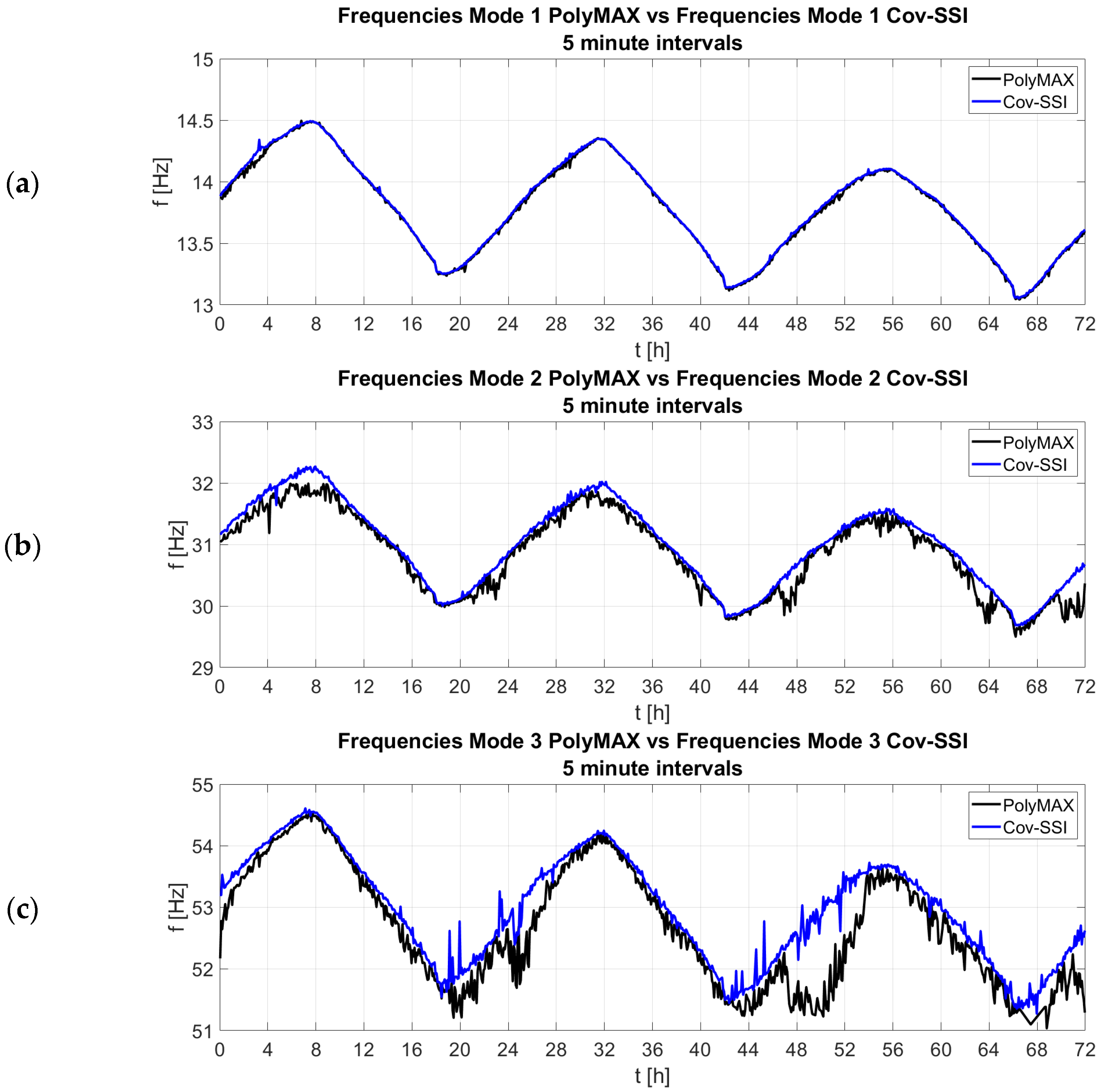
The frequency graphs in the function of time for the 72 h interval obtained with the Cov-SSI method and the PolyMAX method for the first three vibration modes are shown in Figure 8.

Both methods can identify the frequencies for the first three vibration modes. Results are more robust than using peak-picking method for Modes 2 and 3, moreover, the frequencies extracted with the Cov-SSI algorithm for Modes 2 and 3 present a lower variance than those extracted with the PolyMAX method. It should be underlined that the structures are very simple and have well separated modes. Such characteristics help the identification remarkably.

The identified frequencies are correlated with the axial force trend and with the temperature trend.

8. Correlation of Natural Frequencies with Temperature and Axial Force

In this section, the effects on the structure of environmental temperature are evaluated, trying to separate frequency variations due to environmental factors from frequency variations due to structural damage.

Very light levels of damage have been introduced to stress the disturbance on the identification coming from environmental parameters.

The correction of the effect of temperature is performed in two different ways: firstly, by using ambient temperature regression; then, by using axial force variation directly measured on each beam as the correction input. This second approach will lead to much better results than the correlation with ambient temperature.

8.1. Regressions between Natural Frequencies and Temperature or Axial Force

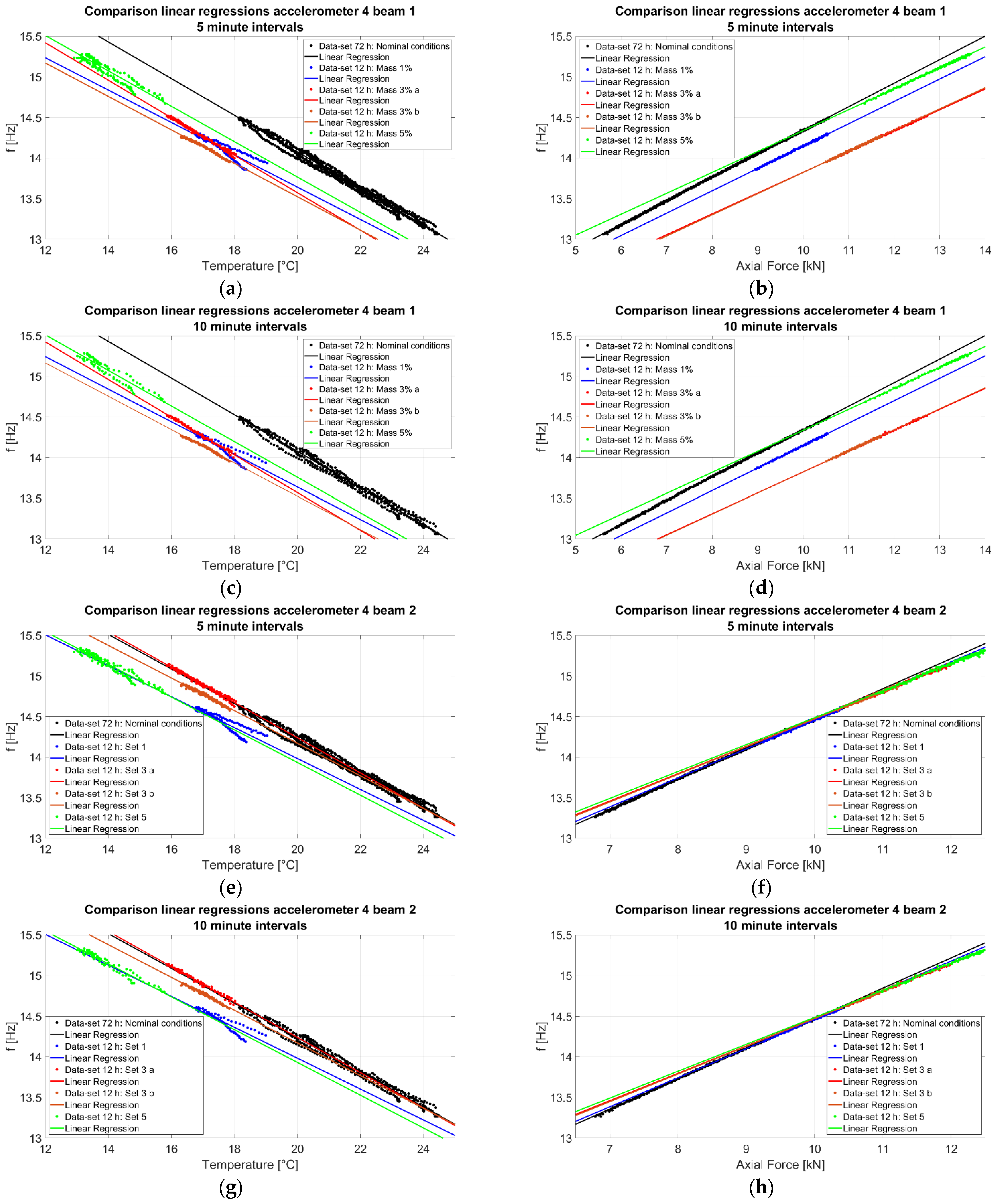
The regressions between the identified raw frequencies and temperature and between the identified raw frequencies and axial force are shown in Figure 9. The raw frequencies used for the graphs are obtained with the peak-picking method for Mode 1. Results of all data sets for the first three vibration modes are similar to those shown in Figure 9, regardless of the adopted approach (peak-picking, Cov-SSI and PolyMAX); therefore, the following considerations can be applied to all results.

The following considerations can be drawn from the linear regression results:

• discretizing the data set in 5-min or 10-min records leads to almost equal correlation results: 10-min records give generally better R² values of the regression than 5-min ones, but the differences are negligible.
• The correlations between ambient temperature and the frequencies show different and distinct regressions for each dataset for both beams.
• The correlations between the axial force and the identified frequencies for Beam 1 present distinct regressions for each dataset, except for the two datasets where the same damage is simulated (same additional mass). Beam 2 (undamaged) shows the same behavior in each dataset. Thus, correlations between axial force and frequencies are much better than correlations between temperature and frequencies, as will be explained in detail in the next paragraph.

8.2. Frequency Correction with Temperature or Axial Force

Raw frequencies can be corrected using temperature regression parameters as follows:

$$f_{c,i}=f_{raw,i}-D_t\left(T_i-T_0\right)$$

(13)

where:

• $f_{c,i}$ is the i-th value of the corrected data set; namely, corrected for temperature effects.
• $f_{raw,i}$ is the i-th raw frequency value.
• $D_t$ is the temperature drift coefficient.
• $T_i$ is the instantaneous temperature.
• $T_0$ is a temperature value chosen as a reference. The average temperature on the 72-h data set has been chosen as the temperature base point, $T_0=21.29 °\mathrm{C}$.

The same parameters $D_t$ and $T_0$, coming from the 72-h dataset (chosen as reference) are then used for the correction of all the other datasets.

Raw frequencies can also be corrected using axial force regression parameters as follows:

$$f_{c,i}=f_{raw,i}-D_f\left(F_i-F_0\right)$$

(14)

where:

• $f_{c,i}$ is the i-th value of the frequency corrected using axial force.
• $f_{raw,i}$ is the i-th raw frequency value.
• $D_f$ is the force drift coefficient.
• $F_i$ is the instantaneous axial force.
• $F_0$ is an axial force value chosen as a reference. The average force on the 72-h data set has been chosen as the force base values $F_0=8.08 \mathrm{kN}$ for Beam 1 and $F_0=8.63 \mathrm{kN}$ for Beam 2.

The same parameters $D_f$ and $F_0$, coming from the 72-h dataset (chosen as reference), are then used for the correction of all the other datasets.

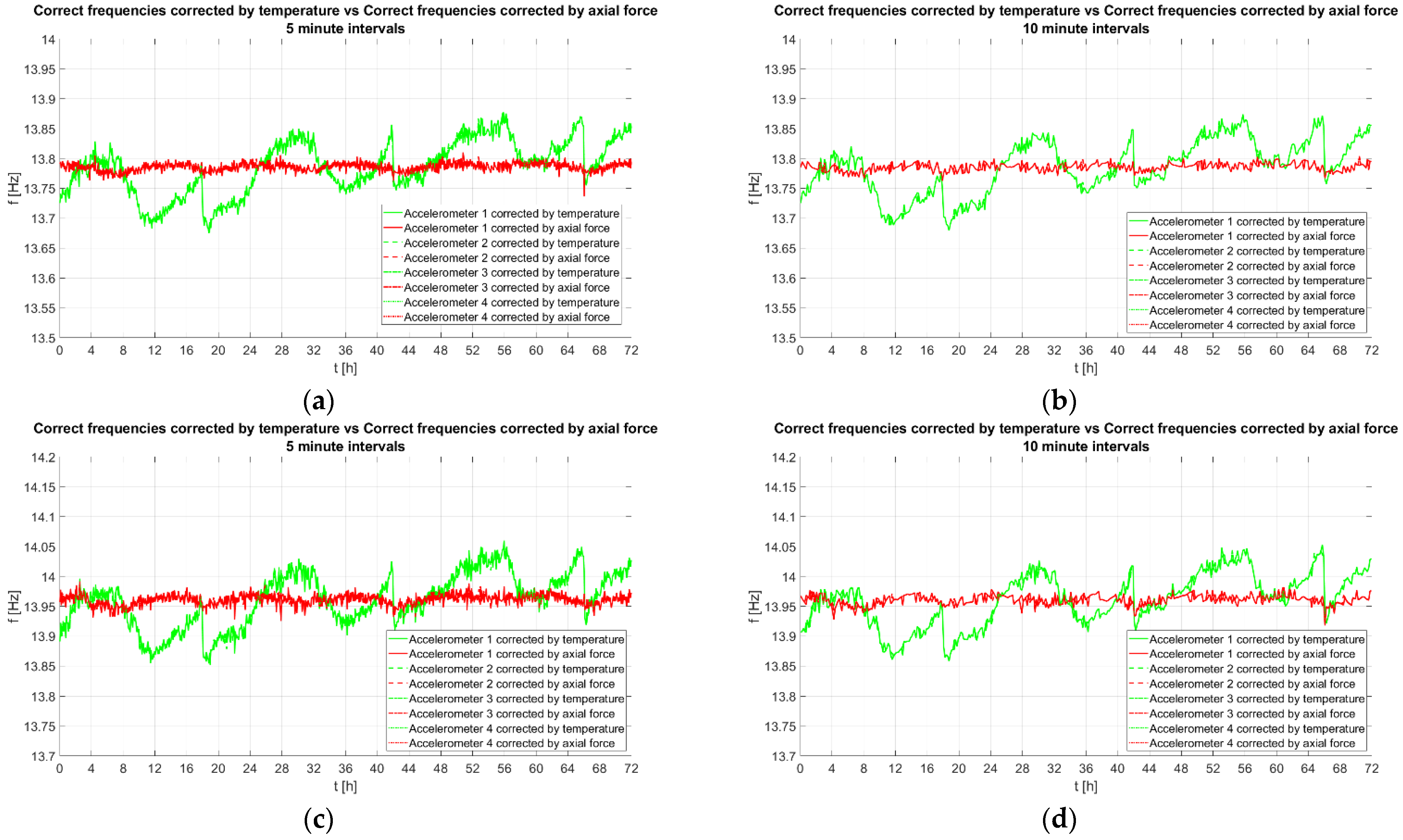
A comparison between frequencies corrected using temperature (green curves) and frequencies corrected using axial force (red curves) is shown in Figure 10. These results are related to the 72-h dataset for Mode 1 frequencies extracted with the peak-picking method. Similar results are obtained for the remaining four datasets for the frequencies of modes higher than the first, and for PolyMAX and Cov-SSI results.

The result of the correction of the raw frequencies using ambient temperature is still strongly correlated to the daily thermal cycles, while the correction using axial force provides a better and more stable result.

In Beam 1, the 72-h dataset corrected with temperature obtains:

• average frequency 13.79 Hz
• maximum frequency 13.88 Hz (+0.7% form average)
• minimum frequency 13.68 (−0.8% from average)

whereas, if axial force is used, the same values are:

• average frequency 13.78 Hz
• maximum frequency 13.81 Hz (+0.1% form average)
• minimum frequency 13.76 (−0.1% from average)

Similar results are obtained for Beam 2.

A comparison of the corrected frequencies over 12 h of the five analyzed datasets is shown in Figure 11 for the results obtained using peak-picking method for Mode 1. Completely similar results are obtained for higher modes with PolyMAX and Cov-SSI.

In Beam 1, where the damage is simulated, the frequencies of Mode 1 decrease depending on the magnitude of damage and its location, as will be discussed in the next paragraph.

In Beam 2, where damage is not present, the force-corrected frequencies lie in a very narrow range of values (red curves), whereas the temperature-corrected frequencies (green curves) show a less stable trend and therefore seem unreliable to detect damage.

8.3. Evaluation of the Effect of Simulated Damage

The following tables quantify the frequency variations between the 12-h datasets and the 72-h dataset that was chosen as benchmark. The variation is the difference between the averages of the corrected frequencies done on the 12-h dataset and on the first 12 h of the 72-h dataset.

The results obtained by applying peak-picking, Cov-SSI and PolyMAX methods are comparable, but peak picking gives clear results only for Mode 1. The differences between datasets discretized in 5-min records and datasets discretized in 10-min records are negligible. The most important difference is between frequency corrections with temperature and with axial force.

Beam 2 is sound in each dataset; therefore, no frequency variation should be appreciated between the 72 h benchmark and the 12 h datasets. When the correction is carried out by using axial force (

Table 4. Beam 2: frequency variation, 5-min intervals discretization, correction with axial force.

	PP	Cov-SSI			PolyMAX
	Mode 1	Mode 1	Mode 2	Mode 3	Mode 1	Mode 2	Mode 3
Set 1	0.0%	0.0%	0.0%	0.0%	−0.1%	0.0%	+0.1%
Set 3a	−0.3%	−0.3%	[-]	−0.2%	−0.1%	[-]	−0.1%
Set 3b	−0.2%	−0.1%	−0.2%	−0.1%	−0.2%	−0.2%	0.0%
Set 5	−0.4%	−0.4%	−0.2%	0.0%	−0.4%	−0.4%	0.0%

and

Table 5. Beam 2: frequency variation, 10-min intervals discretization, correction with axial force.

	PP	Cov-SSI			PolyMAX
	Mode 1	Mode 1	Mode 2	Mode 3	Mode 1	Mode 2	Mode 3
Set 1	−0.1%	0.0%	−0.1%	0.0%	−0.1%	0.0%	+0.1%
Set 3a	−0.3%	−0.3%	[-]	−0.2%	−0.2%	[-]	−0.3%
Set 3b	−0.2%	−0.1%	−0.2%	−0.1%	−0.2%	−0.2%	−0.1%
Set 5	−0.5%	−0.4%	0.0%	0.0%	−0.4%	−0.3%	−0.2%

), the absolute maximum frequency variation between the different datasets is smaller than 0.5%; this result is in line with what expected, since Beam 2 remains in nominal conditions in each dataset. When the correction is carried out using ambient temperature (

Table 6. Beam 2: frequency variation, 5-min intervals discretization, correction with temperature.

	PP	Cov-SSI			PolyMAX
	Mode 1	Mode 1	Mode 2	Mode 3	Mode 1	Mode 2	Mode 3
Set 1	−2.0%	−2.0%	−1.6%	−1.2%	−2.0%	−1.6%	−1.2%
Set 3a	+0.3%	+0.3%	[-]	+0.2%	+0.5%	[-]	+0.2%
Set 3b	−0.6%	−0.5%	−0.5%	−0.3%	−0.6%	−0.6%	−0.2%
Set 5	−2.5%	−2.5%	−1.9%	−1.3%	−2.4%	−2.1%	−1.4%

and

Table 7. Beam 2: frequency variation, 10-min intervals discretization, correction with temperature.

	PP	Cov-SSI			PolyMAX
	Mode 1	Mode 1	Mode 2	Mode 3	Mode 1	Mode 2	Mode 3
Set 1	−1.9%	−2.0%	−1.7%	−1.2%	−2.1%	−1.6%	−1.3%
Set 3a	+0.4%	+0.3%	[-]	+0.2%	+0.4%	[-]	+0.1%
Set 3b	−0.4%	−0.5%	−0.5%	−0.3%	−0.6%	−0.4%	−0.4%
Set 5	−2.4%	−2.5%	−1.9%	−1.3%	−2.4%	−2.0%	−1.6%

), wider spreads can be observed, up to 2.5%.

In the set 3a dataset, no results were obtained for Mode 2 due to the interference caused by a neighboring laboratory test. The neighboring fatigue test produced a forcing with a frequency close to the second mode of vibration of the beam. Therefore, for the entire duration of the sampling, for Mode 2, values at a constant frequency of 33.75 Hz were obtained. Consequently, it was not possible to correlate the frequencies with either temperature or axial force.

In case of “Mass 1%” tests, Beam 1 has a fixed mass of 1% in midspan. A frequency variation on Mode 1 of 0.0% ÷ 0.1% on the sound beam (Table 4 and Table 5) and of −1.3% ÷ −1.4% on the damaged beam (

Table 8. Beam 1: frequency variation, 5-min intervals discretization, correction with axial force.

	PP	Cov-SSI			PolyMAX
	Mode 1	Mode 1	Mode 2	Mode 3	Mode 1	Mode 2	Mode 3
Mass 1%	−1.4%	−1.4%	0.0%	−0.6%	−1.3%	+0.3%	−0.6%
Mass 3% a	−4.2%	−4.2%	[-]	−2.5%	−4.1%	[-]	−2.5%
Mass 3% b	−4.0%	−4.1%	−0.2%	−2.5%	−3.9%	+0.1%	−2.7%
Mass 5%	−0.7%	−0.7%	−1.1%	−2.1%	−0.6%	−0.6%	−2.6%

and

Table 9. Beam 1: frequency variation, 10-min intervals discretization, correction with axial force.

	PP	Cov-SSI			PolyMAX
	Mode 1	Mode 1	Mode 2	Mode 3	Mode 1	Mode 2	Mode 3
Mass 1%	−1.4%	−1.4%	−0.1%	−0.6%	−1.3%	+0.3%	−0.6%
Mass 3%a	−4.2%	−4.2%	[-]	−2.6%	−4.1%	[-]	−2.5%
Mass 3%b	−4.0%	−4.1%	−0.2%	−2.5%	−3.9%	0.1%	−2.7%
Mass 5%	−0.7%	−0.7%	−1.1%	−2.2%	−0.5%	−0.5%	−2.1%

) is appreciated by all methods using the correction with axial force. It can be therefore be estimated that the additional 1% mass causes a variation of the first mode frequency of −1.2% ÷ −1.4%.

When the correction is performed using ambient temperature, the difference can rise to −1.9% ÷ −2.1% on the sound beam (Table 6 and Table 7) and to −3.3% ÷ −3.5% on the damaged beam (

Table 10. Beam 1: frequency variation, 5-min intervals discretization, correction with temperature.

	PP	Cov-SSI			PolyMAX
	Mode 1	Mode 1	Mode 2	Mode 3	Mode 1	Mode 2	Mode 3
Mass 1%	−3.5%	−3.4%	−1.7%	−1.8%	−3.4%	−1.2%	−1.9%
Mass 3%a	−3.4%	−3.4%	[-]	−2.1%	−3.3%	[-]	−2.1%
Mass 3%b	−4.2%	−4.4%	−0.4%	−2.6%	−4.2%	−0.2%	−2.9%
Mass 5%	−2.4%	−2.4%	−2.5%	−3.1%	−2.3%	−1.9%	−3.3%

and

Table 11. Beam 1: frequency variation, 10-min intervals discretization, correction with temperature.

	PP	Cov-SSI			PolyMAX
	Mode 1	Mode 1	Mode 2	Mode 3	Mode 1	Mode 2	Mode 3
Mass 1%	−3.3%	−3.5%	−1.7%	−1.8%	−3.4%	−1.2%	−1.9%
Mass 3%a	−3.2%	−3.4%	[-]	−2.1%	−3.3%	[-]	−2.0%
Mass 3%b	−4.1%	−4.4%	−0.4%	−2.6%	−4.2%	−0.1%	−2.9%
Mass 5%	−2.3%	−2.4%	−2.5%	−3.2%	−2.3%	−1.8%	−3.2%

). The compensation with ambient temperature provides an initial error on the frequency of about −2%; this is greater than the effect of 1% mass in midspan (1.3% to 1.5% of variation on frequency). Therefore, the introduction of this mass cannot be clearly appreciated if frequency correction is done using ambient temperature. A limit in detecting a structural change due to the imperfect environmental effects correction is therefore recognized.

In case “Mass 3%”, Beam 1 has a fixed mass of 3% in midspan. When correction with axial force is done, a frequency variation on Mode 1 of −0.1% ÷ 0.3% on the sound beam (Table 4 and Table 5) and of −3.9% ÷ −4.2% on the damaged beam (Table 8 and Table 9), can be appreciated by all methods. Therefore, it can be estimated that the additional mass causes a variation of the frequency of the first mode of −3.6% ÷ −4.1%; this is about 3 times that measured for 1% additional mass.

When the correction is performed using ambient temperature, the frequency variation is −0.6% ÷ +0.5% on the sound beam (Table 6 and Table 7) and −3.3% ÷ −4.4% on the damaged beam (Table 10 and Table 11). Therefore, it can be estimated that the frequency variation of the first mode, visible after temperature compensation, is −2.7% ÷ −4.9% (less accurate than −3.6% ÷ −4.1% estimated with axial force compensation).

In case “Mass 5%”, Beam 1 has a fixed mass of 5% at L/10. The most accurate predictions can be done observing Mode 3.

A frequency variation on Mode 3 of 0.0% ÷ −0.2% on the sound beam (Table 4 and Table 5) and of −2.1% ÷ −2.6% on the damaged beam (Table 8 and Table 9) can be appreciated by Cov-SSI and PolyMAX methods using the correction with axial force. Therefore, it can be estimated that the additional 5% mass at L/10 causes a variation of the frequency of the third mode of −1.9% ÷ −2.6%.

When the correction is performed using ambient temperature, the difference can rise to −1.3% ÷ −1.6% on the sound beam (Table 6 and Table 7) and to −3.1% ÷ −3.3% on the damaged beam (Table 10 and Table 11). The compensation with ambient temperature provides an initial frequency spread of about −1.45%; this is large if compared with the effect of the mass −1.5% ÷ −2.0%. Therefore, the introduction of this mass cannot be clearly appreciated if frequency correction is done using ambient temperature.

9. Conclusions

The present work aims to highlight the limits of structural health monitoring techniques based on the analysis of output-only data from an accelerometer network, when the variation of the frequencies of the monitored system is used as the only indicator of damage. The main cause found to limit the effectiveness of OMA are thermal disturbances.

Three of the most common OMA methods are applied to the same experimental data to obtain a comparative assessment and to study the effect of ambient parameters (temperature) on the output of the methods.

Longer sampling (10 min instead of 5 min) provides slightly better results because of the higher dynamic information content, but the difference is almost negligible for all the three methods used. Therefore, using 5-min signals as input could be useful to shorten the calculation time.

The application of the peak-picking method is successful only for the first mode of vibration which is easier to excite with environmental vibrations. However, the peak-picking method is useful for preliminary analysis of sampled signals. It allows an initial assessment of the sampled data, a qualitative evaluation of the system’s own frequencies and an initial understanding of the system’s behavior.

For high-order modes, the excitation due to environmental vibrations is lower and the system’s own modes begin to be confused within the ambient noise. The limitations shown by the peak-picking method can also be related to the fact that no optimization for PSD evaluation was performed. The focus was on obtaining their maximum frequency resolution. In addition, optimization would require the evaluation of PSDs on discretization intervals different from those chosen and working well with the other methods. Therefore, a comparison between the peak-picking method and the other two methods would not have been possible.

The other two methods, Cov-SSI and PolyMAX, can provide good results for modes higher than the first.

Three different simulated damages on one beam are identified with different degrees of accuracy, depending on the cleaning procedure of the signal from temperature drift.

A result of considerable interest is the difference between the results obtained performing correction of the raw frequency data using a mechanical parameter (the tensile force in the rods) and the results obtained using ambient temperature correction.

In the case of correction with ambient temperature, the results show a highly variable trend over time; on the contrary, when the correction is done using the axial forces in the rods, the results are significantly stable over time.

Cleaning of the raw frequencies by means of a parameter not measured directly on the beam, such as ambient temperature, leads to variability in the results which can hide the presence of damage on the specimens.

In the presented experimental campaign, the vibration of the rods is influenced by a single parameter affected by temperature: the axial force. This is a very simple case, as the specimens’ geometry is extremely simple. Moreover, the presence of a load cell and strain gauges allows to directly measure this parameter on both rods, therefore cleaning the frequency response using a parameter that is not available for more complex real structures in the field.

In real SHM cases [27,28,29,30,31], when bridges or historical buildings are under investigation, the frequency response of the structure is not related to a single mechanical parameter (axial force); therefore, it is usually not possible to measure physical parameters that are as good as the axial force in controlling the test results, as is the case in the present work.

Therefore, the frequency correction is commonly done using environmental temperature, or in the best situations, using the temperature obtained by thermocouples fixed on the surfaces of the structure. The data coming from real-life SHM applications are then more similar to those obtained from the experimental dataset of this campaign corrected with ambient temperature.

Therefore, it is extremely difficult to assess small damages causing frequency variations close to those caused by ambient temperature.

The following key points emerge from the study reported in this paper:

• Mechanical models (such as F.E.M) are very useful to check the results obtained from operational modal analysis. In the study reported in this paper, the knowledge of the theoretical frequencies was very important to be able to exclude non-physical modes and external forcing (the fatigue test).
• The peak-picking method is only effective for identifying the frequency of the first mode of vibration, as the signal–to–noise ratio was very low, whereas Cov-SSI and PolyMAX provide better and more robust results.
• The correction of frequency data using ambient temperature is not entirely effective and leads to results affected by a variability that can have an order of magnitude similar to the effect of the damage that need to be individuated.

In SHM applications of structures like bridges or buildings, it is therefore very important to evaluate the data provided by OMA techniques with care, as they are highly affected by external environmental factors.

In many cases the damages that are under investigation generate very little frequency variation in serviceability conditions (especially in prestressed concrete structures); thus, they can be easily hidden within the thermal noise. Damage such as reinforcement corrosion in prestressed structures can in fact generate sensible reduction of bearing capacity with very small reduction of stiffness; therefore, generating very small frequency variation.

For these reasons, OMA techniques are undoubtedly useful for dynamic identification, but their limits in open field use should be assessed with care to avoid misleading results.