Continuous Latent Spaces Sampling for Graph Autoencoder

Abstract

This paper proposes colaGAE, a self-supervised learning framework for graph-structured data. While graph autoencoders (GAEs) commonly use graph reconstruction as a pretext task, this simple approach often yields poor model performance. To address this issue, colaGAE employs mutual isomorphism as a pretext task for a continuous latent space sampling GAE (colaGAE). The central idea of mutual isomorphism is to sample from multiple views in the latent space and reconstruct the graph structure, with significant improvements in terms of the model’s training difficulty. To investigate whether continuous latent space sampling can enhance GAEs’ learning of graph representations, we provide both theoretical and empirical evidence for the benefits of this pretext task. Theoretically, we prove that mutual isomorphism can offer improvements with respect to the difficulty of model training, leading to better performance. Empirically, we conduct extensive experiments on eight benchmark datasets and achieve four state-of-the-art (SOTA) results; the average accuracy rate experiences a notable enhancement of $0.3\%$, demonstrating the superiority of colaGAE in node classification tasks.

1. Introduction

GNNs have achieved remarkable success in recent years, particularly in the domain of graph-structured data such as biochemistry, physics, and social science data [1,2,3]. However, a major limitation of GNNs is that they require a significant amount of manually labeled data during training [4]. In many real-world scenarios, labeled information is scarce and expensive, which makes it difficult to meet the demands of large-scale data [5,6]. To overcome this limitation, the clever integration of GNNs with semi-supervised learning (SSL) has become a powerful solution for unsupervised graph representation learning. These solutions include GCL (such as Deep Graph Infomax (DGI) [7], Graph Contrastive Coding (GCC) [8], Bootstrapped Graph Representation Learning (BGRL) [9], GRAph Contrastive rEpresentation learning (GRACE) [4], and Graph Contrastive learning with Adaptive augmentation (GCA) [10]) and GAE (such as Variational Graph Auto-Encoders (VGAE) [11], Self-Supervised Masked Graph Autoencoders (GraphMAE) [12], Masked Graph Autoencoders (MaskGAE) [13], Adversarially Regularized Graph Autoencoder (ARVGA) [14], and Multi-View Graph Representation MVGRL [15]).

These methods transform the nodes, edges, or subgraphs of a graph into low-dimensional embeddings via an unsupervised objective (preprocessing task), such as graph reconstruction tasks [11]. This approach preserves critical information, such as the structure and topology of the graph, to learn widely useful representations from unlabeled graphs in a task-agnostic manner [16].

However, the success of GCL comes at the cost of relatively complex training strategies [12]. To stabilize the training process, GCL typically requires momentum updates and exponential moving averages [8,9]. Moreover, most contrastive objectives require negative samples, which often need to be sampled or constructed from graphs, such as GRACE [4], GCA [10], and DGI [17], requiring a considerable amount of labor. Finally, the heavy reliance of contrastive SSL on high-quality data augmentation proves to be a pain point, such as in the case of CCA-SSG [18], as the effectiveness of graph augmentation heuristics varies drastically across different graphs.

Fortunately, graph autoencoders (GAEs) naturally avoid the aforementioned issues in the reconstruction approach, as their learning objective is to directly recover the input graph data [11]. Specifically, GAEs use node embeddings to train an encoder and expect to reconstruct the adjacency matrix of the input graph from a decoder-based representation, thereby preserving topological proximity and enhancing representation learning [13]. Compared to GCL, GAEs are typically relatively simple to implement and easy to integrate with existing frameworks, as they naturally treat graph reconstruction as a preprocessing task without the need for view generation augmentation.

However, the simplicity of GAE is its curse as well, as it can lead to poor model performance. Compared to the fancy objectives and complex structures of GCL, their pre-processing tasks are few and simple [19]. Previous GAEs have mainly used masking to increase the model’s training difficulty. This work proposes using graph isomorphism as a pretext task to increase the model’s training difficulty. The most common principles of graph reconstruction may overly emphasize prior information, and are not always beneficial [20]. For example, while most GAEs utilize link reconstruction as an objective to promote topological proximity among neighbors, they may perform poorly on node and graph classification tasks. Additionally, feature reconstruction without corruption may not be robust enough [4]. For GAEs utilizing feature reconstruction, most use plain architectures, which can lead to the risk of learning trivial solutions [13]. We believe that this is because previous GAEs have only sampled within a single latent space, making models prone to overfitting.

To address this issue, we propose colaGAE, which involves training multiple encoders. Although training a single encoder is easy for neural networks, training multiple encoders becomes challenging. The outputs of these encoders are mutually isomorphic and can be used as a preprocessing task to train the encoder. We conduct extensive empirical experiments on eight benchmark datasets, demonstrating that colaGAE outperforms several state-of-the-art models on node classification tasks.

The main contribution of this paper is to propose a pretext task for GAEs using graph isomorphism. As an unsupervised learning model, GAEs have been widely applied in various fields such as computer vision, natural language processing, recommendation systems, bioinformatics, and clustering analysis. Graph contrastive learning has significant application value in different domains, where it can assist researchers in better understanding and processing various types of graph data. Our proposed model achieves four state-of-the-art results out of eight datasets without the addition of any other techniques or tricks while using a regular GCN as the base model. This demonstrates that using graph isomorphism as a proxy task for GAEs is effective in improving model performance. This enables models to learn better node representations, resulting in better downstream task performance.

The present work first introduces the concept and algorithm of a GNN based on SSL (see Section 2), followed by the introduction of related background knowledge in Section 3. Building on the above sections, colaGAE is proposed in Section 4, and experimental results, including ablation studies (see Section 7), are presented in Section 5. Finally, in Section 8, the advantages and limitations of colaGAE are thoroughly discussed, and a summary and future outlook are provided.

2. Related Work

This section provides a brief introduction to the fundamental concepts and principles of SSL-based graph neural networks in order to help readers gain a rapid understanding of how graph neural networks operate.

2.1. Graph Neural Networks

The objective of a GNN is to utilize the graph structures and node features to learn representations of the nodes. To achieve this, GNNs typically follow a two-step processing approach consisting of aggregation and feature transformation. In the first step, the representations of a selected node and its neighboring nodes are combined through aggregation. In the second step, these aggregated representations are mapped into a new feature space via a shared linear transformation, followed by an update operation [21,22]. However, using a complete graph as input is often necessary to achieve this, which, due to hardware resource constraints, limits the applicability of these methods to large-scale graph data. To address this issue, GraphSAGE [23] iteratively samples subgraphs for aggregation and updating. Nonetheless, most existing methods [24] rely on external guidance, such as annotated labels, which restricts their applicability.

2.2. Graph Contrastive Learning

The primary objective of Graph Contrastive Learning (GCL) is to learn embeddings that bring positive samples closer to one another while simultaneously separating them from negative samples. GCL has been adapted from various domains, such as computer vision and natural language processing. For instance, DGI [17] uses mutual information maximization as a pretext task [25] to train models, while MVGRL [15] is based on graph diffusion [26] and extends CMC [27] to graphs. GCC [8] integrates InfoNCE [28] and MoCo [29] for large-scale Graph Neural Network (GNN) pretraining. Other GCL approaches, such as SimCLR [30], GRACE [4], GCA [10], and GraphCL [20], directly consider other nodes/graphs as negative samples to learn node/graph representations. BGRL [9], inspired by BYOL [31], adopts a negative-sample-free pretext task with complex asymmetric architectures. Additionally, MERIT [32] uses self-distillation and performs contrastive learning, while AFGRL [33] treats nodes as positive samples by considering their context without augmentation or negative sampling.

2.3. Graph AutoEncoders

GAEs are a common component of GNNs, and typically consist of an encoder and a decoder. The encoder maps nodes to low-dimensional representations, while the decoder reconstructs the original graph. Recent approaches have demonstrated the effectiveness of GAEs in modeling node relationships and learning robust representations from graphs by following the autoencoding philosophy [14]. For instance, VGAE [11] uses missing edge prediction as its pretext task, while GraphMAE and MaskGAE [12,13] focus on masking and recovering node and edge features. GPT-GNN [34] proposes an autoregressive framework to perform iterative node and edge reconstruction, while ARVGA [14] focuses primarily on link prediction and graph clustering objectives. Moreover, MVGRL [15] seeks global-level information over graphs with persistence.

3. Preliminaries

A graph with N nodes and M edges can be represented as $\mathcal{G}=\{\mathcal{V},\mathcal{E}\}$, where $\mathcal{V}$ is the node set ${\left\{v_i\right\}}_{i=1}^N$ and $\mathcal{E}$ is the edge set ${\left\{e_i\right\}}_{i=1}^M$. Let $A\in {\{0,1\}}^{N\times N}$ be the adjacency matrix of graph $\mathcal{G}$; ${\mathit{A}}_{ij}=1$ if and only if $(v_i,v_j)\in \mathcal{E}$, where $(v_i,v_j)$ represents the existence of an edge between node $v_i$ and node $v_j$. To prevent isolated nodes during training, $\tilde{A}$ stands for the adjacency matrix for a graph with added self-loops $\mathbf{I}$; each node $v_i\in \mathcal{V}$ is associated with a d-dimensional feature vector $x_i\in {\mathbb{R}}^d$. Hence, for simplicity, an attributed graph can be described as $\mathcal{G}=(\mathbf{X},A)$. Graph $\mathcal{G}$ is isomorphic to graph ${\mathcal{G}}^{\prime }$, and we use $\mathcal{G}\sim {\mathcal{G}}^{\prime }$ to represent this relation. What is more, the isomorphism is transitive; if ${\mathcal{G}}_1\sim {\mathcal{G}}_2$ and ${\mathcal{G}}_2\sim {\mathcal{G}}_3$, then according to transitivity, ${\mathcal{G}}_1\sim {\mathcal{G}}_3$. GAEs learn a parametric mapping function $f_{\theta }$ that transfers the node feature matrix X into low-dimensional latent representations $\mathbf{Z}$; formally, $f_{\theta }\left(\mathcal{G}\right)=\mathbf{Z}\in {\mathbb{R}}^{N\times d}$.

4. Present Work: colaGAE

4.1. Motivation

The pretext task is a crucial aspect of graph SSL. In this section, we explain why mutual isomorphism represents a novel approach to the pretext task.

GNNs are designed to extract valuable information from raw data and create representations that are generalizable, transferable, and robust. However, aggregating node features using a single latent space may not be enough. This perspective is supported by the attention mechanism, demonstrated in the work of Vaswani et al. [35]. The attention mechanism is a way of expressing the same entity in different latent spaces. Each attentional head in the model represents a unique latent space. For instance, in BERT [36], each of the twelve attention heads produces a 64-dimensional vector, which are concatenated into a final 768-dimensional vector.

The node representations are then used to reconstruct the graph structure A. A recent study shows that simple MLPs distilled from trained GNN teachers perform comparably to advanced GNNs on node classification [37]. This suggests that the graph’s topological structure can be effectively integrated into node-level features as prior information. In other words, promising node representations can accurately recover the graph’s topological structure.

In summary, node representations are obtained by synthesizing multiple continuous latent spaces and can recover the graph’s structure. To achieve node-level representations from different latent spaces, we propose a series-encoder to generate various outputs. The series-encoder consists of a series of encoders, where each output is isomorphic to the adjacency matrix under the same graph. Because of the transductive nature of isomorphism, all outputs are mutually isomorphic. Therefore, mutual isomorphism is an inherent natural property of the series-encoder, and can serve as the pretext task.

4.2. Encoder

The colaGAE method we propose employs a series-encoder that produces a sequence of outputs, denoted as $Z_1,Z_2,\cdots ,Z_n$, where each encoder is trained with a distinct mapping function $f_i$, as illustrated in Equation (1).

$$Z_i=f_i\left(\mathcal{X}\right)$$

(1)

The low-dimensional latent representations, denoted by $\mathbf{Z}$, are subsequently inputted into the decoder to reconstruct the original graph, as described in Equation (2).

$${\widehat{G}}_i=Dec\left({\mathbf{Z}}_i\right)$$

(2)

In this research, we discovered that the decoder’s design plays a critical role in learning expressive and informative node representations. Because the goal of feature reconstruction is to learn such representations, rather than simply matching the encoded embeddings to the input node features, we opted for an MLP decoder. This type of decoder is more likely to reconstruct a node’s original feature from its encoded embedding.

The encoder in colaGAE consists of five different feature extractors, including GCN, which are widely used in GNN research and have demonstrated effectiveness in various graph-related tasks. Additionally, we included four linear mapping layers that produce node representations of the same shape. Although our framework can accommodate different encoder architectures, such as GraphSAGE and GAT, we chose GCN because of its simplicity, efficiency, and ability to address the scalability issue in pretraining large GNNs.

4.3. Decoder

The decoding process in our proposed colaGAE method involves combining pairwise node embeddings into a representation of the links in the graph. The type of decoder used is determined by the approach used for aggregation, such as the inner product decoder and linear mapping decoder. To simplify our method and highlight the impact of mutual-isomorphism, we chose a decoder that does not require parameters. Thus, we define the decoder in the following way:

$$Dec\left(\mathbf{Z}\right)=\langle \mathbf{Z},{\mathbf{Z}}^T\rangle ={\mathbf{Z}}^{\mathrm{T}}\mathbf{Z}$$

(3)

Here, $\langle \mathbf{Z},{\mathbf{Z}}^T\rangle$ represents the inner product of $\mathbf{Z}$, which indicates the cosine similarity between nodes. Theoretically, all of the decoder’s outputs are isomorphic to the adjacency matrix A. Formally, $Dec\left({\mathbf{Z}}_n\right)\sim Dec\left({\mathbf{Z}}_{n-1}\right)\sim \cdots \sim Dec\left({\mathbf{Z}}_0\right)\sim A$.

4.4. Learning Objective

The measurements used to represent nodes in our proposed colaGAE method have two components, namely, distribution and Euclidean distance. We assume that the outputs from each encoder are isomorphic to one another, ensuring consistency in distribution and noticeable clustering in Euclidean distance. To reflect these properties, we propose two learning objectives.

4.5. Reconstruction Loss

The reconstruction loss, denoted as ${\mathcal{L}}_{\mathrm{RE}}$, measures how well the model can reconstruct the original graph structure in terms of edges. To calculate this loss, we use a graph autoencoder, which has an encoder that maps input features $\mathcal{X}$ to hidden representations $\mathcal{Z}$, and a decoder, which maps it back to reconstruct the adjacency matrix A of the graph. We calculate the reconstruction error using the mean squared error (MSE), denoted as $\mathbf{MSE}$, as shown in Equation (4).

$$\mathbf{MSE}=\frac{1}{n^2}\sum _{i,j}{(Dec\left({\mathbf{Z}}_{i,j}\right)-{\mathit{A}}_{i,j})}^2$$

(4)

Using the MSE can lead to near-zero values, which is not desirable, as the concept of “lengths of edges” is not a topology-based concept. As a solution, we use the binary cross-entropy (BCE), which determines whether there is an edge or not between two nodes, instead. The BCE is used to calculate the reconstruction error; thus, the reconstruction loss is a combination of both MSE and BCE, as shown in Equation (6).

$$BCE=\frac{-1}{N^2}\sum A·logDec\left(\mathbf{Z}\right)+(1-A)·(1-logDec\left(\mathbf{Z}\right))$$

(5)

Using the BCE loss is a way to measure the model’s ability in order to predict whether or not there is an edge between two nodes in the graph. This loss treats each entry in the adjacency matrix as a binary classification problem, and encourages the model to learn to predict the correct label for each edge in the graph instead of merely minimizing the difference between predicted and actual edge weights. By combining the MSE and BCE losses, it is possible to train a model that captures the structure of the graph while ensuring the correct presence or absence of edges.

$${\mathcal{L}}_{\mathrm{RE}}=\mathbf{MSE}(Dec\left(\mathbf{Z}\right),A)+\mathbf{BCE}(Dec\left(\mathbf{Z}\right),A)$$

(6)

4.6. Relative Distance Loss

The way nodes in a graph are arranged is often reflected by the tendency of nodes to cluster together. This clustering tendency is commonly measured using the Euclidean distance, where nodes that are close to each other are considered neighbors. However, using the mean square error (MSE) as a measure may not be appropriate for graph data, which often have low density and a degree distribution that follows a power law. This can lead to high-degree and low-degree nodes coexisting, making the assumption of Euclidean spaces invalid and the optimization process ineffective.

To address this issue, we propose a new loss function that takes distance as a relative concept. Unlike deep clustering methods, which require maximizing mutual information or manually selecting cluster centers, our approach aims to bring neighboring nodes closer while pushing non-neighboring nodes farther apart. Specifically, we introduce the Relative Distance (RD) loss function, which is defined as follows:

$${\mathcal{L}}_{\mathrm{RD}}=-log\frac{{\sum }_{(i,j)\in E}Dec({\mathbf{Z}}_i,{\mathbf{Z}}_j)}{{\sum }_{(i,j)\notin E}Dec({\mathbf{Z}}_i,{\mathbf{Z}}_j)}$$

(7)

In (7), the set E represents the edges in the graph, while $Dec({\mathbf{Z}}_i,{\mathbf{Z}}_j)$ denotes the distance between two nodes i and j, computed by the decoding function $Dec$. The numerator and denominator in the RD loss function correspond to the respective sums of the distances between neighboring and non-neighboring nodes. Minimizing the numerator and maximizing the denominator results in neighboring nodes being pulled closer together while non-neighboring nodes are pushed further apart. This is achieved without the need for mutual information maximization or cluster center selection, making the RD loss function an effective way to model the clustering tendency of graph data.

4.7. Training and Evaluating Setups

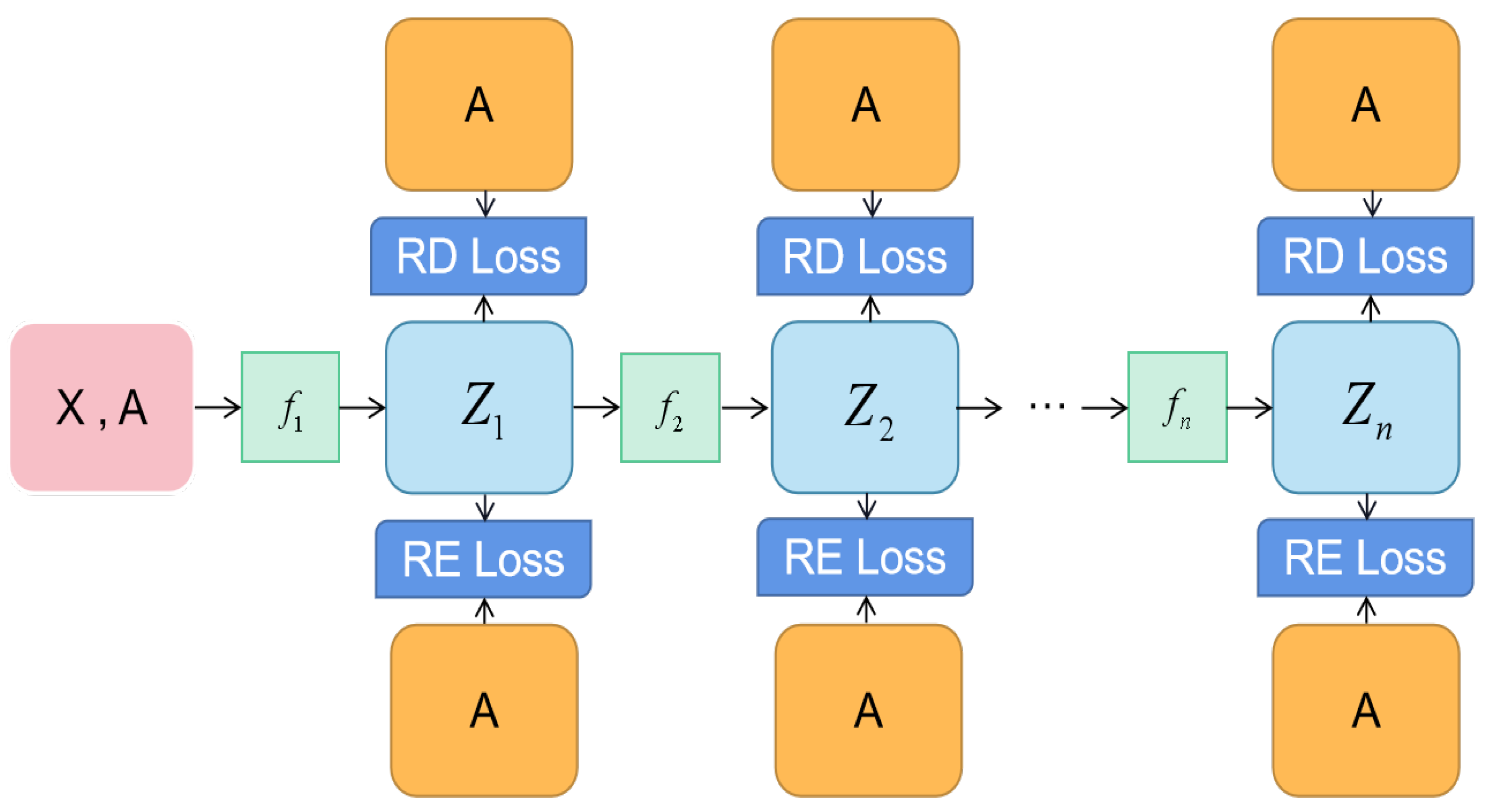
The task of node classification involves predicting labels for unknown nodes. We evaluated the performance of our proposed colaGAE on eight standard benchmarks, including Cora, Citeseer, PubMed, and Ogbn-arxiv. These benchmarks are citation networks in which nodes represent documents and edges represent citations. The overall training process is summarized in Figure 1.

The framework consists of a series of encoders, denoted as $f_0$ to $f_n$, where $f_0$ is a GCN encoder and $f_1$ to $f_n$ are MLP encoders. The first encoder, $f_0$, has a significant impact on performance, and we refer to it as “the first encoder” in subsequent sections for convenience. These encoders continuously encode node representations from one latent space into another, which can be viewed as a continuous sampling from different semantic spaces. Overall, colaGAE is a simple and effective framework for self-supervised graph autoencoder learning.

First, we feed the entire graph $\mathcal{G}=(\mathbf{X},A)$ into the series-encoder to generate different representations.

In order to evaluate the effectiveness of the node representations learned by our model in reconstructing the adjacency matrix A, we utilize both the reconstruction loss and relative distance loss, as outlined in Algorithm 1. The hyperparameters $\alpha$ and $\beta$ are used to adjust the weighting of these criteria in the overall performance of the model.

Algorithm 1: Pseudocode of colaGAE in Pytorch-like style.

# A: adjacency matrix # alpha: coefficient of reconstruction loss # beta: coefficient of relative distance loss # model: GCN + mlp layers   class encoder():     def _ _init_ _(self, n_layers = 1):         super(encoder, self)._ _init_ _()         basic_block = [             Linear(), Sigmoid(), BatchNorm1d()         ]         basic_block *= n_layers         self.proj = nn.Sequential(∗basic_block)     def forward(self, x):         x = self.proj(x)         return x   def reconstruction_loss(z,A):     zz = [email protected]     loss = F.mse_loss(zz,A)     loss += F.binary_cross_entropy_with_logits(zz,A)     return loss   def relative_distance_loss(z,A):     distance = [email protected]     loss = (distance∗A).sum() / (distance∗(1-A)).sum()     return -torch.log(loss)   # to deal with large graphs, we need to sample their subGraphs for subGraph in Graph:     # transfer subGraphs into low-dimensional representation     z0 = GCN(subGraph)     z1 = encoder(z0) ; z2 = encoder(z1)     z3 = encoder(z2) ; z4 = encoder(z3)     z5 = encoder(z4) ; z6 = encoder(z5)     z7 = encoder(z6) ; z8 = encoder(z7)       loss = 0     for z in [z0,z1,z2,z3,z4]:           # A_sub is the adjacency graph of the subGraph         re_loss = reconstruction_loss(z,A_sub)         rd_loss = relative_distance_loss(z,A_sub)           # add losses         loss += alpha∗re_loss + beta∗rd_loss       # Adam optimizer     loss.backward()     update(model.params)   with torch.no_grad():     evaluation(model)

Graph data are typically sparse, with a density defined as $\frac{2E}{N(N-1)}$, where E is the number of edges and $N(N-1)$ is the maximum number of edges in a graph with N nodes. In contrast to text data, which often contain dense information, the densities of the Cora, Citeseer, and Pubmed datasets (see

Table 1. Statistics of benchmark datasets.

Dataset	Nodes	Edges	Classes	Features	Density
Cora	2708	10,556	7	1433	0.288%
Citeseer	3327	9228	6	3703	0.167%
Pubmed	19,717	88,651	3	500	0.046%
CS	18,333	327,576	15	6805	0.195%
Computer	13,752	574,418	10	767	0.608%
Photo	7650	287,326	8	745	0.982%
Arxiv	169,343	1,166,243	40	128	0.008%
MAG	1,939,743	21,111,007	349	128	0.001%

) are only $0.288\%$, $0.167\%$, and $0.046\%$, respectively. Due to this sparsity, the concatenated node-level representations from the series-encoder as output do not provide satisfactory results. Errors accumulate from $\mathbf{Z}0$ to $\mathbf{Z}n$ during training, with $Dec\left(\mathbf{Z}n\right)\sim A\Rightarrow Dec\left(\mathbf{Z}0\right)\sim A$. However, the reverse is not necessarily true, indicating that $\mathbf{Z}0$ is more robust than $\mathbf{Z}n$. Hence, we use only ${\mathbf{Z}}_0$ for evaluations and downstream tasks, especially for the node classification task in this paper.

After training, all encoders in the series-encoder except for the first can be discarded. This approach enables colaGAE to be used with any other graph SSL methods. Additionally, by replacing the encoder in the first layer of the series-encoder (e.g., replacing GCN with GraphSAGE), our colaGAE can be used with large graphs.

In conclusion, our proposed colaGAE is a straightforward and scalable self-supervised graph learning framework. Algorithm 1 provides the pseudocode for the model algorithm.

5. Experiments

5.1. Datasets

• Cora, Citeseer, and Pubmed: [21]: three standard citation networks in which nodes are documents and edges indicate citation relations. In the experiments, they are employed for node classification (transductive) and clustering tasks.
• Computer and Photo: Amazon Computers and Amazon Photo are segments of the Amazon co-purchase graph, where nodes represent goods, edges indicate that two goods are frequently purchased together, node features are bag-of-words encoded product reviews, and class labels are provided by the product category.
• Coauthor CS: Coauthor CS is co-authorship graph based on the Microsoft Academic Graph from the KDD Cup 2016 challenge. Here, nodes are authors, which are connected by an edge if they co-authored a paper, node features represent paper keywords for each author’s papers, and class labels indicate the most active fields of study for each author.
• arxiv and MAG: The obgn-arxiv and ogbn-mag datasets are two large datasets from Open Graph Benchmark [38]. The datasets are collected from real-world networks belonging to different domains. Each node is associated with a 128-dimensional word2vec feature vector, and all the other types of entities are not associated with input node features.

The datasets used in the experiments are detailed in Table 1.

5.2. Compared Methods

To demonstrate the effectiveness of our proposed approach, we conducted experiments to compare it with eight other state-of-the-art self-supervised graph learning methods, namely, DGI [17], MVGRL [15], GMI [39], GRACE [4], SUGRL [40], GraphMAE [12], and MaskGAE [13]. As our paper focuses on the node classification downstream task, we included five representative supervised node classification methods as baselines for evaluation as well, namely, MLP, GCN, and GAT.

5.3. Training and Evaluating Setups

The objective of the node classification task is to predict labels for unknown nodes in a given network. In this study, we evaluated the performance of colaGAE on eight standard benchmarks that cover both transductive and inductive scenarios. These benchmarks include Cora, Citeseer, PubMed, and Ogbn-arxiv, which are citation networks in which nodes represent documents and edges represent citations.

The network architecture of colaGAE comprises a series-encoder with the same structure as illustrated in Figure 1. The first layer of the series-encoder is GCN, followed by [1, 2, 3, 4, 5] layers of linear mappings, each equipped with batch normalization [41] and a sigmoid activation function. We used different numbers of hidden units for each dataset. The dropout rate between each layer was carefully tuned within the range of [0, 0.1, 0.2, 0.3, 0.4].

For each dataset, we used Adam as the optimizer for 500 fixed training iterations. In addition, we performed a hyperparameter search for the learning rate within the range of [0.001, 0.01, 0.05, 0.1] and a weight decay within the range of [5 × 10⁻⁴, 5 × 10⁻³]. We employed an early stopping strategy with a patience of 50, i.e., we stopped training when the validation metric did not improve for 50 epochs.

To ensure consistency with previous research in the field [9,15,18,22], we followed standard evaluation protocols in our experiments. We used publicly available data splits for the Cora, Citeseer, PubMed, Arxiv, and MAG datasets. For the remaining three datasets, we used a 1:1:8 training, validation, and testing split. We trained a linear classifier based on the best-performing model as determined by the validation results and kept the classifier parameters fixed while generating embeddings for all nodes. Finally, we report the average test node accuracy over 20 random initializations.

5.4. Software and Hardware Infrastructures

Our framework is built upon PyTorch and Deep Graph Library, which are open-source software. All datasets used throughout the experiments are publicly available and do not have licenses. All experiments were performed on a single GeForce RTX 2080Ti GPU with 11 GB memory.

5.5. Results

We compared our colaGAE approach with several SOTA graph SSL models; as presented in

Table 2. Node classification accuracy (%) on eight benchmark datasets. In each column, the boldfaced score denotes the best result and the underlined score represents the second-best result.

	Cora	CiteSeer	PubMed	Photo	Computer	arXiv	MAG	Coauthor-CS
MLP	47.90$\pm 0.40$	49.30$\pm 0.30$	69.10$\pm 0.20$	78.50$\pm 0.20$	73.80$\pm 0.10$	56.30$\pm 0.30$	22.10$\pm 0.30$	90.37$\pm 0.00$
GCN	81.50$\pm 0.20$	70.30$\pm 0.40$	79.00$\pm 0.50$	92.42$\pm 0.22$	86.51$\pm 0.54$	70.40$\pm 0.30$	30.10$\pm 0.30$	90.52$\pm 0.21$
GAT	83.00$\pm 0.70$	72.50$\pm 0.70$	79.00$\pm 0.30$	92.56$\pm 0.35$	86.93$\pm 0.29$	70.60$\pm 0.30$	30.50$\pm 0.30$	91.10$\pm 0.10$
DGI	82.30$\pm 0.60$	71.80$\pm 0.70$	76.80$\pm 0.60$	91.61$\pm 0.22$	83.95$\pm 0.47$	65.10$\pm 0.40$	31.40$\pm 0.30$	92.15$\pm 0.63$
GMI	83.00$\pm 0.30$	72.40$\pm 0.10$	79.90$\pm 0.20$	90.68$\pm 0.17$	82.21$\pm 0.31$	68.20$\pm 0.20$	29.50$\pm 0.10$	-
GRACE	81.90$\pm 0.40$	71.20$\pm 0.50$	80.60$\pm 0.40$	92.15$\pm 0.24$	86.25$\pm 0.25$	68.70$\pm 0.40$	31.50$\pm 0.30$	90.10$\pm 0.80$
GCA	81.80$\pm 0.20$	71.90$\pm 0.40$	81.00$\pm 0.30$	92.53$\pm 0.16$	87.85$\pm 0.31$	68.20$\pm 0.20$	31.40$\pm 0.30$	93.08$\pm 0.18$
MVGRL	82.90$\pm 0.30$	72.60$\pm 0.40$	80.10$\pm 0.70$	91.70$\pm 0.10$	86.90$\pm 0.10$	68.10$\pm 0.10$	31.60$\pm 0.40$	92.11$\pm 0.12$
BGRL	82.86$\pm 0.49$	71.41$\pm 0.92$	82.05$\pm 0.85$	93.17$\pm 0.30$	90.34$\pm 0.19$	71.64$\pm 0.12$	31.11$\pm 0.11$	93.3$\pm 0.11$
SUGRL	83.40$\pm 0.50$	73.00$\pm 0.40$	81.90$\pm 0.30$	93.20$\pm 0.40$	88.90$\pm 0.20$	69.30$\pm 0.20$	32.40$\pm 0.10$	92.20$\pm 0.50$
CCA-SSG	83.59$\pm 0.73$	73.36$\pm 0.72$	80.81$\pm 0.38$	93.14$\pm 0.14$	88.74$\pm 0.28$	52.55$\pm 0.10$	23.39$\pm 0.63$	93.06$\pm 0.03$
GAE	74.90$\pm 0.40$	65.60$\pm 0.50$	74.20$\pm 0.30$	91.00$\pm 0.10$	85.10$\pm 0.40$	63.60$\pm 0.50$	27.10$\pm 0.30$	90.01$\pm 0.71$
VGAE	76.30$\pm 0.20$	66.80$\pm 0.20$	75.80$\pm 0.40$	91.50$\pm 0.20$	85.80$\pm 0.30$	64.80$\pm 0.20$	27.90$\pm 0.20$	92.11$\pm 0.09$
ARGA	77.95$\pm 0.70$	64.44$\pm 1.19$	80.44$\pm 0.74$	91.82$\pm 0.08$	85.86$\pm 0.11$	67.34$\pm 0.09$	28.36$\pm 0.12$	90.09$\pm 0.33$
ARVGA	79.50$\pm 1.01$	66.03$\pm 0.65$	81.51$\pm 1.00$	91.51$\pm 0.09$	86.02$\pm 0.11$	67.43$\pm 0.08$	28.32$\pm 0.18$	91.21$\pm 0.57$
GraphMAE	84.20$\pm 0.40$	73.40$\pm 0.40$	81.10$\pm 0.40$	92.86$\pm 0.17$	88.06$\pm 0.23$	71.75$\pm 0.17$	31.67$\pm 0.34$	92.89$\pm 0.43$
MaskGAE	84.05$\pm 0.18$	73.49$\pm 0.59$	83.06$\pm 0.22$	93.09$\pm 0.06$	89.51$\pm 0.08$	70.73$\pm 0.30$	32.79$\pm 0.26$	93.00$\pm 0.15$
colaGAE	84.23$\pm 0.07$	73.61$\pm 0.05$	83.33$\pm 0.10$	93.00$\pm 0.11$	90.05$\pm 0.04$	72.21$\pm 0.15$	31.09$\pm 0.12$	93.07$\pm 0.11$

, the results demonstrate that our approach achieves either the best or competitive performance compared to existing models. Our approach outperforms the previous best SOTA on four out of eight datasets by a small margin, with an average improvement of approximately 0.4%. Specifically, on the first three datasets, we observe an average relative improvement of 0.2% over the previous SOTA.

Previous research has suggested that GCLs outperform GAEs due to the limited available pretext tasks in GAEs. However, the success of our colaGAE model demonstrates that mutual isomorphism is a promising pretext task for GAEs. The results suggest that leveraging topological information plays a more crucial role in graph SSL.

We note that CCA-SSG performs poorly on arXiv and MAG, as it is essentially a dimension reduction method, where the ideal embedding dimension should be smaller than the input one, as reported in [18].

During evaluation, colaGAE functions as a GCN-encoder while outperforming all baselines. Notably, colaGAE surpasses supervised GCN by an average of approximately 2.5%, indicating that prior information such as graph topological structure is critical for graph SSL. Its downstream performance on the large arXiv and MAG datasets further verifies the effectiveness of our colaGAE model.

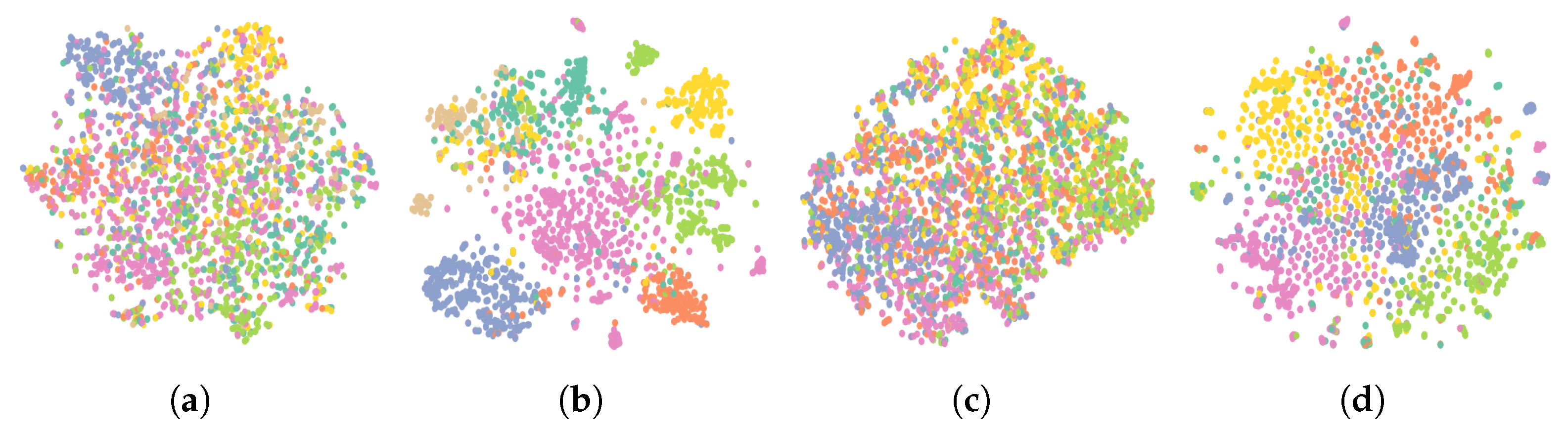
We used t-SNE to visually demonstrate the effectiveness of the node embeddings learned by our proposed model. To provide a comparative analysis, we generated embeddings from the supervised GCN. The results are presented in Figure 2, where each dot corresponds to the embedding of a node and the color represents its true label. Our analysis indicates that our proposed model can identify classes more accurately than the supervised GCN, as the boundaries between different classes are much clearer in the former.

6. Performance Comparison on Link Prediction

Link prediction tasks involve predicting whether an edge exists between two nodes based on incomplete topological information. To perform these tasks, we followed the conventional learning-based approach to link prediction [11] and conducted experiments on three datasets: Cora, CiteSeer, and PubMed. In our experiments, we removed 5% of edges for validation and 10% for testing. We reported the AUC score and average precision (AP) and compared our results against other algorithms. As shown in

Table 3. Link prediction results (%) on the three citation networks.

	Cora		CiteSeer		PubMed
	AUC	AP	AUC	AP	AUC	AP
GAE	91.09$\pm 0.01$	92.83$\pm 0.03$	90.52$\pm 0.04$	91.68$\pm 0.05$	96.40$\pm 0.01$	96.50$\pm 0.02$
VGAE	91.40$\pm 0.01$	92.60$\pm 0.01$	90.80$\pm 0.02$	92.00$\pm 0.02$	94.40$\pm 0.02$	94.70$\pm 0.02$
ARGA	92.40$\pm 0.00$	93.23$\pm 0.00$	91.94$\pm 0.00$	93.03$\pm 0.00$	96.81$\pm 0.00$	97.11$\pm 0.00$
ARVGA	92.40$\pm 0.00$	92.60$\pm 0.00$	92.40$\pm 0.00$	93.00$\pm 0.00$	96.50$\pm 0.00$	96.80$\pm 0.00$
SAGE	86.33$\pm 1.06$	88.24$\pm 0.87$	85.65$\pm 2.56$	87.90$\pm 2.54$	89.22$\pm 0.87$	89.44$\pm 0.82$
MGAE	95.05$\pm 0.76$	94.50$\pm 0.86$	94.85$\pm 0.49$	94.68$\pm 0.34$	98.45$\pm 0.03$	98.22$\pm 0.05$
colaGAE	96.37$\pm 0.51$	96.24$\pm 0.46$	98.01$\pm 0.52$	97.92$\pm 0.30$	98.46$\pm 0.27$	98.19$\pm 0.31$

, our proposed model outperformed all other compared algorithms, demonstrating its superior performance in link prediction tasks.

7. Ablation Study

In order to gain a deeper insight into the working of our proposed model, we conducted several ablation studies to explore the influence of crucial components, such as the embedding size, number of layers, and encoder, on the node classification task. We systematically varied one component at a time while keeping the others fixed at their optimal values, then evaluated the performance of our proposed model accordingly.

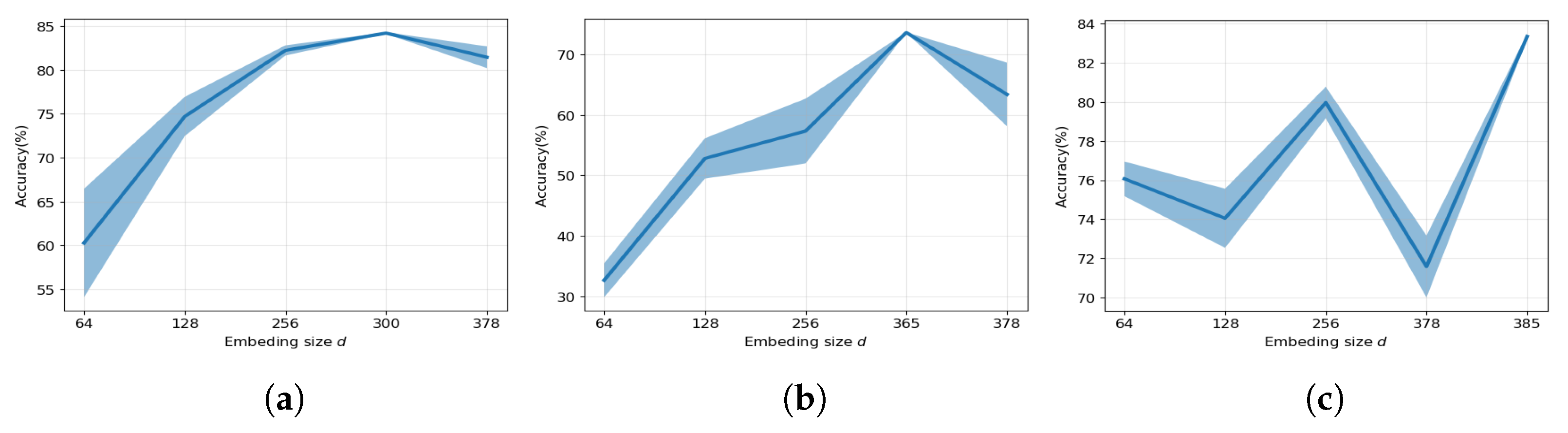
7.1. Effect of Embedding Size

The impact of varying the embedding size on the performance of our proposed model is illustrated in Figure 3. The embedding size is a critical factor in graph representation learning, as it reflects the efficacy of information compression. Our results indicate that our proposed model benefits significantly from a larger embedding dimension, with its performance generally improving as the embedding size increases in most cases. This is consistent with the methods reported in [40], which typically require larger dimensions (e.g, 512) to achieve their best performance.

For instance, considering the Cora dataset, we observed that our proposed model achieved its best performance at a 300-dimensional embedding size, whereas DGI and GIM achieved their best performance at a 512-dimensional embedding size. This suggests that even though 300-dimensional embeddings are relatively small compared to 512-dimensional embeddings, they are nearly as effective. This may indicate that information compression plays a crucial role in graph autoencoder models, and that higher information density leads to higher performance.

7.2. Effect of the Number of Layers

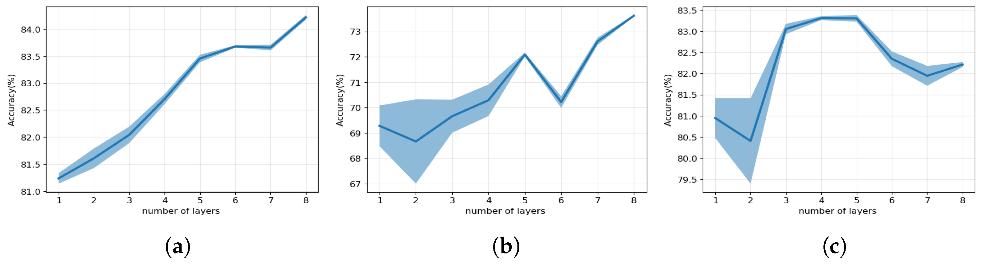
To better understand the practical implementation of mutual isomorphism, we conducted a series of experiments to investigate the impact of the number of layers on the performance of our colaGAE model. This is important because mutual isomorphism is a theoretical concept that poses significant challenges in its practical implementation. As shown in Figure 4, our findings reveal that increasing the number of layers in the series-encoder leads to consistent improvements in the performance of colaGAE across the three benchmark datasets used in the experiment. This observation further affirms the validity of the mutual isomorphism assumption.

Moreover, it is notable that the performance of colaGAE becomes more stable as the number of layers increases, while the standard deviation decreases. This suggests that increasing the number of layers helps to delineate classification boundaries more precisely, contributing to the model’s enhanced performance.

7.3. Effect of Encoders

We conducted additional experiments to explore whether different encoders could improve the performance of our proposed model. As shown in

Table 4. Statistics showing the effects of different encoders. The results were produced by replacing the first encoder of colaGAE model’s series-encoder.

Dataset	MLP	GCN	GAT	GraphSAGE	GRACE
Cora	72.51	84.23	84.43	83.97	85.14
Citeseer	65.41	73.61	72.19	73.81	74.08
Pubmed	80.19	83.33	82.90	82.65	84.11

, the results indicate that the choice of encoder has a significant effect on the model’s performance. Specifically, using negative samples in GRACE improves the quality of learned representations for downstream tasks.

It is noteworthy that GRACE leverages negative samples, which may explain why it achieves the best performance on all three datasets as an encoder.

8. Conclusions

In this paper, we discuss the limitations of self-supervised GAEs and attribute their poor performance to the restrictive pretext tasks they are subjected to. These limitations result in simplistic structures and easy convergence, ultimately leading to inferior performance compared to GCL models. To address this issue, we propose a novel pretext task for graph semi-supervised learning—mutual isomorphism—which employs a sequence encoder structure to increase the difficulty of learning node representations from node features, thereby improving the model’s performance. However, the downside of this method is the requirement for more memory. One solution to this issue could be to convert the graph reconstruction problem into an edge existence problem and train the model using sampling. This aspect of the work will be addressed in future research.

References

- Senior, A.W.; Evans, R.; Jumper, J.; Kirkpatrick, J.; Sifre, L.; Green, T.; Qin, C.; Žídek, A.; Nelson, A.W.; Bridgland, A.; et al. Improved protein structure prediction using potentials from deep learning. Nature 2020, 577, 706–710. [Google Scholar] [CrossRef] [PubMed]
- Shlomi, J.; Battaglia, P.; Vlimant, J.R. Graph neural networks in particle physics. Mach. Learn. Sci. Technol. 2020, 2, 021001. [Google Scholar] [CrossRef]
- Hamilton, W.L. Graph Representation Learning. Synth. Lect. Artif. Intell. Mach. Learn. 2020, 14, 1–159. [Google Scholar]
- Zhu, Y.; Xu, Y.; Yu, F.; Liu, Q.; Wu, S.; Wang, L. Deep graph contrastive representation learning. arXiv 2020, arXiv:2006.04131. [Google Scholar]
- Hu, W.; Liu, B.; Gomes, J.; Zitnik, M.; Liang, P.; Pande, V.; Leskovec, J. Strategies for pre-training graph neural networks. arXiv 2019, arXiv:1905.12265. [Google Scholar]
- Sun, F.Y.; Hoffman, J.; Verma, V.; Tang, J. InfoGraph: Unsupervised and Semi-supervised Graph-Level Representation Learning via Mutual Information Maximization. In Proceedings of the ICLR, New Orleans, LA, USA, 6–9 May 2019. [Google Scholar]
- Velickovic, P.; Fedus, W.; Hamilton, W.L.; Liò, P.; Bengio, Y.; Hjelm, R.D. Deep Graph Infomax. ICLR (Poster) 2019, 2, 4. [Google Scholar]
- Qiu, J.; Chen, Q.; Dong, Y.; Zhang, J.; Yang, H.; Ding, M.; Wang, K.; Tang, J. GCC: Graph Contrastive Coding for Graph Neural Network Pre-Training. In Proceedings of the KDD, Virtual Event, 23–27 August 2020. [Google Scholar]
- Thakoor, S.; Tallec, C.; Azar, M.G.; Munos, R.; Veličković, P.; Valko, M. Bootstrapped representation learning on graphs. In Proceedings of the ICLR 2021 Workshop on Geometrical and Topological Representation Learning, Virtual Event, 3–7 May 2021. [Google Scholar]
- Zhu, Y.; Xu, Y.; Yu, F.; Liu, Q.; Wu, S.; Wang, L. Graph contrastive learning with adaptive augmentation. In Proceedings of the Web Conference 2021, Ljubljana, Slovenia, 19–23 April 2021; pp. 2069–2080. [Google Scholar]
- Kipf, T.N.; Welling, M. Variational graph auto-encoders. arXiv 2016, arXiv:1611.07308. [Google Scholar]
- Hou, Z.; Liu, X.; Dong, Y.; Wang, C.; Tang, J.; Wang, C.; Tang, J. GraphMAE: Self-Supervised Masked Graph Autoencoders. arXiv 2022, arXiv:2205.10803. [Google Scholar]
- Li, J.; Wu, R.; Sun, W.; Chen, L.; Tian, S.; Zhu, L.; Meng, C.; Zheng, Z.; Wang, W. MaskGAE: Masked Graph Modeling Meets Graph Autoencoders. arXiv 2022, arXiv:2205.10053. [Google Scholar]
- Pan, S.; Hu, R.; Long, G.; Jiang, J.; Yao, L.; Zhang, C. Adversarially regularized graph autoencoder for graph embedding. arXiv 2018, arXiv:1802.04407. [Google Scholar]
- Hassani, K.; Khasahmadi, A.H. Contrastive multi-view representation learning on graphs. In Proceedings of the International Conference on Machine Learning, PMLR, Virtual Event, 13–18 July 2020; pp. 4116–4126. [Google Scholar]
- Wu, L.; Lin, H.; Tan, C.; Gao, Z.; Li, S.Z. Self-supervised learning on graphs: Contrastive, generative, or predictive. arXiv 2021, arXiv:2105.07342. [Google Scholar] [CrossRef]
- Veličković, P.; Fedus, W.; Hamilton, W.L.; Liò, P.; Bengio, Y.; Hjelm, R.D. Deep Graph Infomax. In Proceedings of the ICLR, New Orleans, LA, USA, 6–9 May 2019. [Google Scholar]
- Zhang, H.; Wu, Q.; Yan, J.; Wipf, D.; Yu, P.S. From canonical correlation analysis to self-supervised graph neural networks. In Proceedings of the NeurIPS, Virtual Event, 6–14 December 2021. [Google Scholar]
- Liu, Y.; Jin, M.; Pan, S.; Zhou, C.; Zheng, Y.; Xia, F.; Philip, S.Y. Graph self-supervised learning: A survey. IEEE Trans. Knowl. Data Eng. 2022, 35, 5879–5900. [Google Scholar] [CrossRef]
- You, Y.; Chen, T.; Sui, Y.; Chen, T.; Wang, Z.; Shen, Y. Graph contrastive learning with augmentations. In Proceedings of the NeurIPS, Virtual Event, 6–12 December 2020. [Google Scholar]
- Kipf, T.N.; Welling, M. Semi-supervised classification with graph convolutional networks. arXiv 2016, arXiv:1609.02907. [Google Scholar]
- Veličković, P.; Cucurull, G.; Casanova, A.; Romero, A.; Lio, P.; Bengio, Y. Graph attention networks. arXiv 2017, arXiv:1710.10903. [Google Scholar]
- Hamilton, W.; Ying, Z.; Leskovec, J. Inductive representation learning on large graphs. Adv. Neural Inf. Process. Syst. 2017, 30, 1–12. [Google Scholar]
- Xu, B.; Shen, H.; Cao, Q.; Qiu, Y.; Cheng, X. Graph Wavelet Neural Network. In Proceedings of the ICLR, New Orleans, LA, USA, 6–9 May 2019. [Google Scholar]
- Hjelm, R.D.; Fedorov, A.; Lavoie-Marchildon, S.; Grewal, K.; Bachman, P.; Trischler, A.; Bengio, Y. Learning deep representations by mutual information estimation and maximization. arXiv 2018, arXiv:1808.06670. [Google Scholar]
- Klicpera, J.; Weißenberger, S.; Günnemann, S. Diffusion improves graph learning. Adv. Neural Inf. Process. Syst. 2019, 32, 13354–13366. [Google Scholar]
- Tian, Y.; Krishnan, D.; Isola, P. Contrastive multiview coding. In Proceedings of the European Conference on Computer Vision, Glasgow, UK, 23–28 August 2020; Springer: Berlin/Heidelberg, Germany, 2020; pp. 776–794. [Google Scholar]
- Oord, A.v.d.; Li, Y.; Vinyals, O. Representation learning with contrastive predictive coding. arXiv 2018, arXiv:1807.03748. [Google Scholar]
- He, K.; Fan, H.; Wu, Y.; Xie, S.; Girshick, R. Momentum contrast for unsupervised visual representation learning. In Proceedings of the IEEE/CVF Conference on Computer Vision and Pattern Recognition, Seattle, WA, USA, 14–19 June 2020; pp. 9729–9738. [Google Scholar]
- Chen, M.; Wei, Z.; Huang, Z.; Ding, B.; Li, Y. Simple and Deep Graph Convolutional Networks. In Proceedings of the International Conference on Machine Learning, PMLR, Online, 13–18 July 2020; pp. 1725–1735. [Google Scholar]
- Grill, J.B.; Strub, F.; Altché, F.; Tallec, C.; Richemond, P.H.; Buchatskaya, E.; Doersch, C.; Pires, B.A.; Guo, Z.D.; Azar, M.G.; et al. Bootstrap your own latent: A new approach to self-supervised learning. arXiv 2020, arXiv:2006.07733. [Google Scholar]
- Jin, M.; Zheng, Y.; Li, Y.F.; Gong, C.; Zhou, C.; Pan, S. Multi-Scale Contrastive Siamese Networks for Self-Supervised Graph Representation Learning. arXiv 2021, arXiv:2105.05682. [Google Scholar]
- Lee, N.; Lee, J.; Park, C. Augmentation-free self-supervised learning on graphs. In Proceedings of the AAAI Conference on Artificial Intelligence, Vancouver, BC, Canada, 20–27 February 2022; Volume 36, pp. 7372–7380. [Google Scholar]
- Hu, Z.; Dong, Y.; Wang, K.; Chang, K.W.; Sun, Y. Gpt-gnn: Generative pre-training of graph neural networks. In Proceedings of the 26th ACM SIGKDD International Conference on Knowledge Discovery & Data Mining, Virtual Event, 6–10 July 2020; pp. 1857–1867. [Google Scholar]
- Vaswani, A.; Shazeer, N.; Parmar, N.; Uszkoreit, J.; Jones, L.; Gomez, A.N.; Kaiser, L.; Polosukhin, I. Attention is all you need. In Proceedings of the Advances in Neural Information Processing Systems, Long Beach, CA, USA, 4–9 December 2017; pp. 5998–6008. [Google Scholar]
- Devlin, J.; Chang, M.W.; Lee, K.; Toutanova, K. Bert: Pre-training of deep bidirectional transformers for language understanding. arXiv 2018, arXiv:1810.04805. [Google Scholar]
- Zhang, S.; Liu, Y.; Sun, Y.; Shah, N. Graph-less Neural Networks: Teaching Old MLPs New Tricks Via Distillation. In Proceedings of the ICLR, Virtual Event, 25–29 April 2022. [Google Scholar]
- Hu, W.; Fey, M.; Zitnik, M.; Dong, Y.; Ren, H.; Liu, B.; Catasta, M.; Leskovec, J. Open graph benchmark: Datasets for machine learning on graphs. Adv. Neural Inf. Process. Syst. 2020, 33, 22118–22133. [Google Scholar]
- Peng, Z.; Huang, W.; Luo, M.; Zheng, Q.; Rong, Y.; Xu, T.; Huang, J. Graph representation learning via graphical mutual information maximization. In Proceedings of the Web Conference 2020, Taipei, Taiwan, 20–24 April 2020; pp. 259–270. [Google Scholar]
- Mo, Y.; Peng, L.; Xu, J.; Shi, X.; Zhu, X. Simple Unsupervised Graph Representation Learning. In Proceedings of the AAAI, Vancouver, BC, Canada, 22 February 2022. [Google Scholar]
- Ioffe, S.; Szegedy, C. Batch Normalization: Accelerating Deep Network Training by Reducing Internal Covariate Shift. In Proceedings of the JMLR Workshop and Conference Proceedings, Lille, France, 6–11 July 2015; Volume 37, pp. 448–456. [Google Scholar]
Figure 1.
The overall framework of colaGAE for SSL on graphs.
Figure 2.
t-SNE analysis, showing a visualization comparison of the node embeddings on the Cora and Citeseer datasets. (a) GCN on Cora; (b) colaGAE on Cora; (c) GCN on Citeseer; (d) colaGAE on Citeseer.
Figure 3.
Effect of embedding size. (a) Cora; (b) Citeseer; (c) Pubmed.
Figure 4.
Effect of the number of layers. (a) Cora; (b) Citeseer; (c) Pubmed.