
Lateral–Torsional Buckling of Cantilever Steel Beams under 2 Types of Complex Loads

Abstract
:1. Introduction
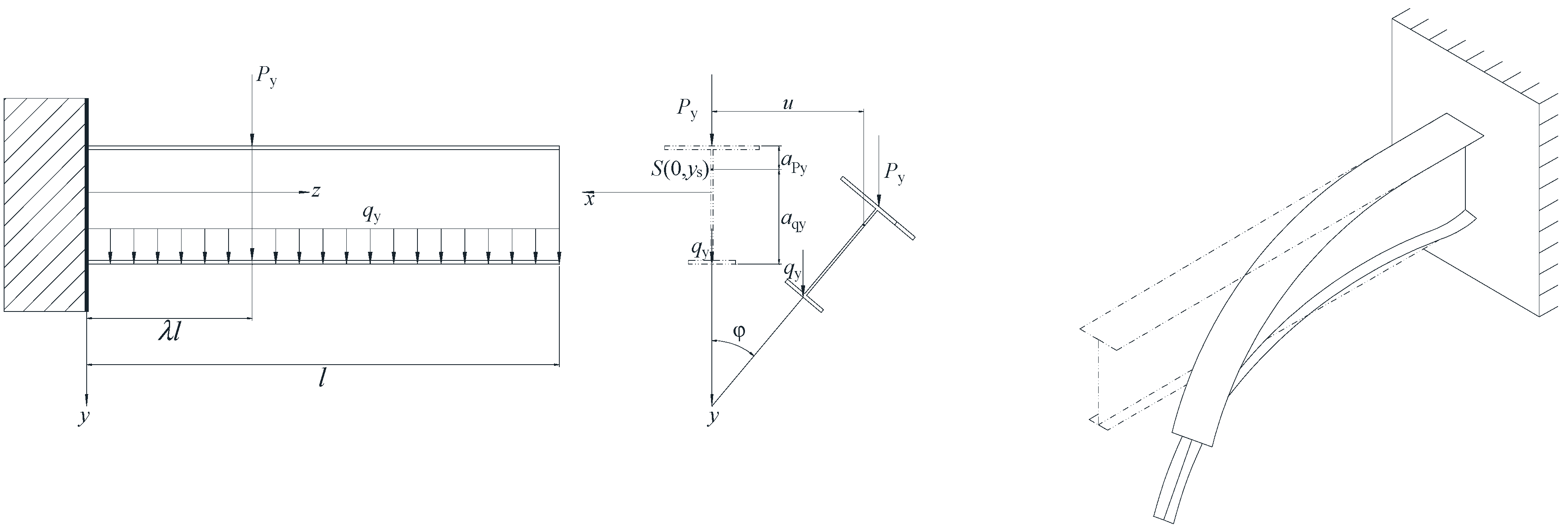
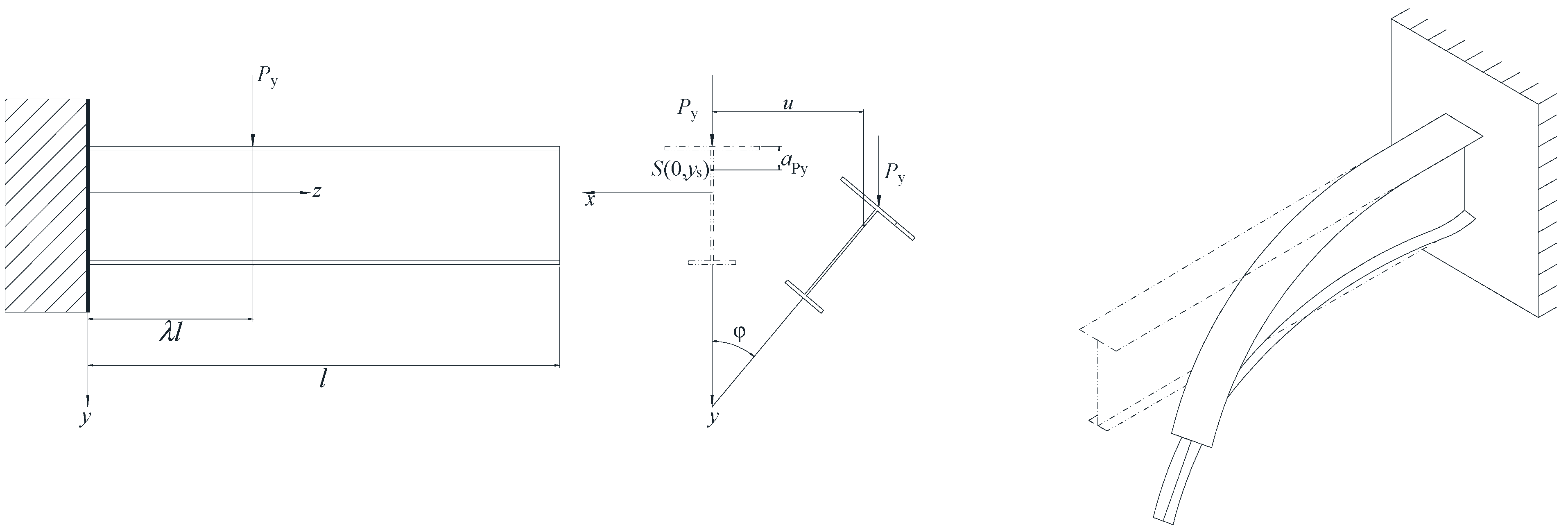
2. Calculation of Total Potential Energy Equation under CL and CUDL
2.1. Introduction and Comparison of Total Potential Energy Equation
2.2. The Buckling Deformation Functions
2.3. Calculation of Total Potential Energy Equation
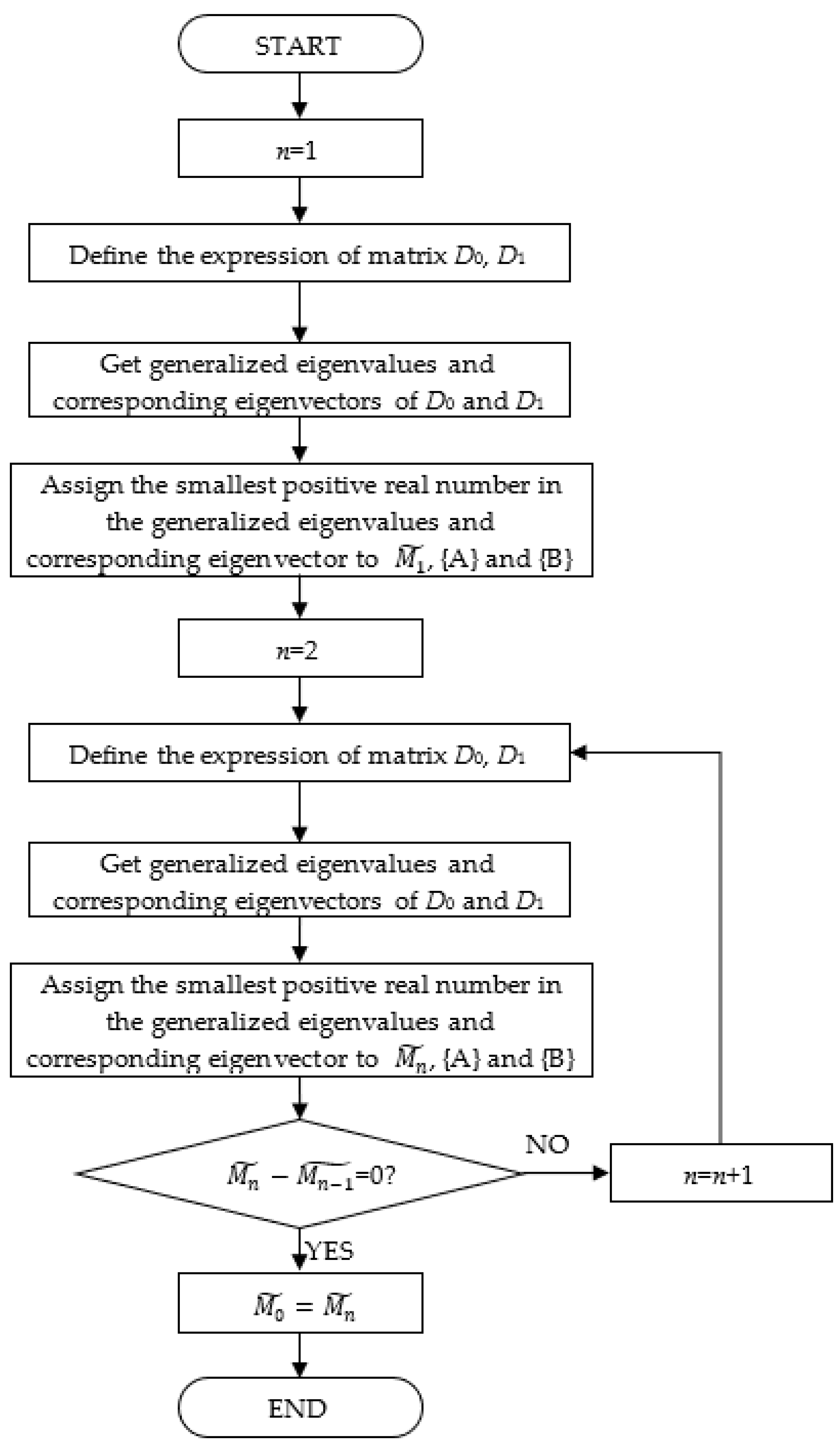
3. Verification and Analysis of Matrix Equation
3.1. Verification of the Results and Discussion
3.2. Comparative Analysis between Matrix Equation and Equations Proposed in Other References
4. Deduction of the Closed-Form Solution of Mcr
4.1. Analysis of the Reason Why Mcr Cannot Be Expressed Accurately by Analytic Expression
4.2. Derivation of Closed-Form Solution of Mcr Based on Twist Angle Function
5. Practical Expressions for Design under CL and CUDL
5.1. Practical Calculation Formula of Mcr
5.2. Example Verification
6. Conclusions
- (1)
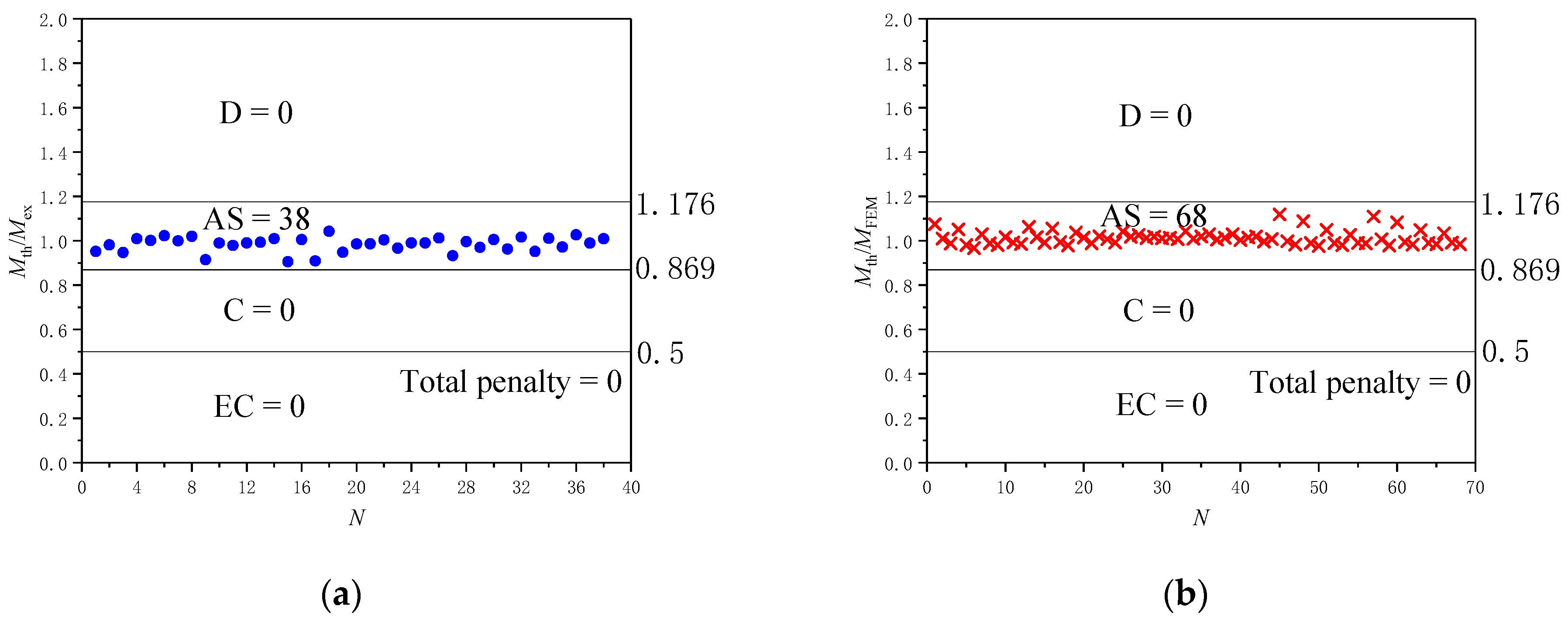
- Mcr and the generalized coordinates An and Bn in the buckling deformation functions of cantilever I-beams under CL and CUDL can be accurately calculated by the numerical method proposed in this paper. Compared with the experimental results and the finite element results of relevant reference, the maximum of the Mth/Mex and Mth/MFEM ratio is 1.07, and the minimum error is 0.92. The average of all the ratios is 0.98 with a standard deviation of 0.13.
- (2)
- The safety, accuracy and economic aspects of the prediction of the numerical method are assessed using DPC. The results show that the numerical method can effectively predict Mcr of cantilever steel beams under CL and CUDL.
- (3)
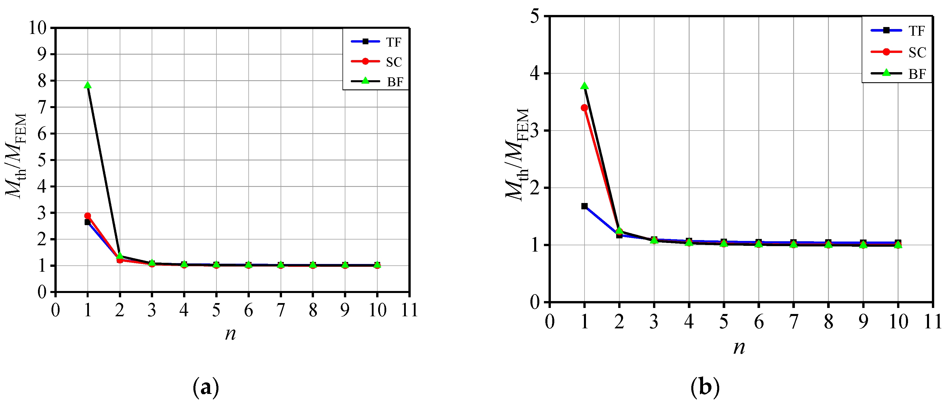
- The number of generalized coordinates determines the accuracy of Mcr. The number of generalized coordinates is defined as n. The obtained errors of Mcr do not exceed 3.96% when n is greater than or equal to 10. The errors of Mcr exceed 17% when n is equal to 1 or 2.
- (4)
- The degree of Mcr in Equation (34) varies with the number of generalized coordinates of twist angle function. When the number of generalized coordinates of twist angle function is n, the degree of Mcr in Equation (34) is 2n.
- (5)
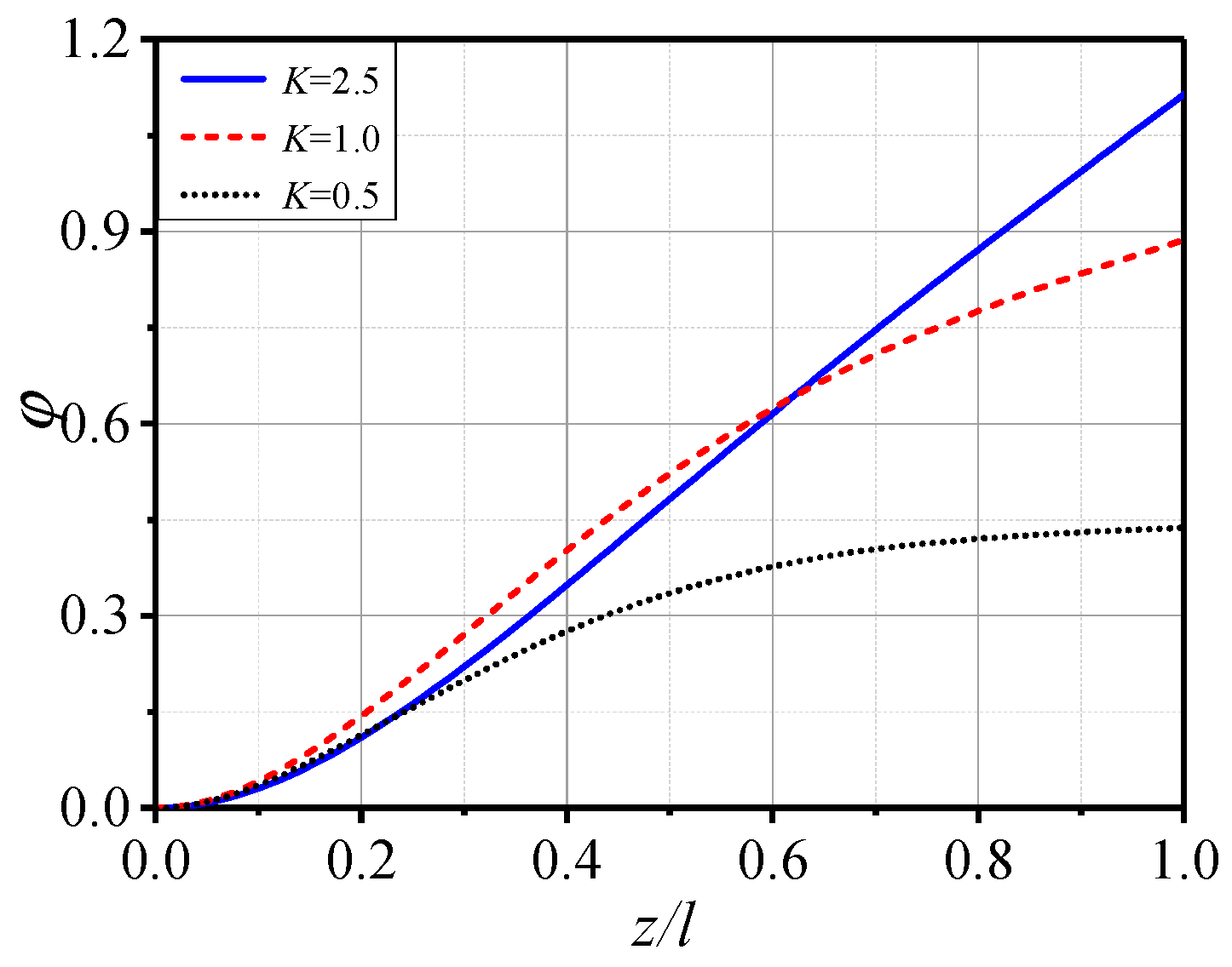
- The torsional buckling mode of the cantilever steel beam is mainly determined by K, which is the torsional stiffness coefficient.
Author Contributions
Funding
Institutional Review Board Statement
Informed Consent Statement
Data Availability Statement
Acknowledgments
Conflicts of Interest
Nomenclature
| LTB | lateral–torsional buckling |
| Mcr | critical moment |
| CL | concentrated load |
| CUDL | combination of concentrated load and uniformly distributed load |
| Cb | lateral–torsional buckling modification factor |
| C1, C2, C3 | correction factor of critical moment |
| l | cantilever length |
| x, y, z | Cartesian coordinates |
| Py, qy | concentrated load and uniformly distributed load |
| aPy, aqy | the difference between the ordinate of load and the ordinate of shear center |
| λ | the ratio of distance between the action point of Py and the fixed end to the cantilever’s length |
| E | Young’s modulus |
| G | shear modulus |
| Iω, It, Iy | warping constant, torsional constant and moment of inertia about y-axis |
| βx | Wagner’s coefficient |
| u, φ | the lateral deflection and twist angle of section |
| u(z), φ(z), φ0(z) | the buckling deformation functions |
| φ(λl) | the twist angle at the point where the transverse concentrated load acts during the lateral–torsional buckling of the beam |
| Mx | the moment about the x-axis |
| α | the ratio of the product of qy multiplied by l to Py |
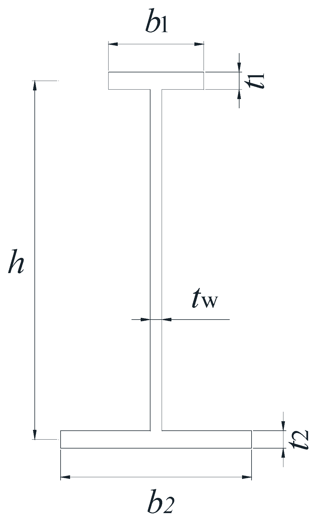
| h | the distance between the centroids of the top and bottom flanges |
| An, Bn | generalized coordinates |
| n, r | the numbers of terms of buckling deformation functions |
| M0, |M0| | the moment when z = 0, the maximum absolute value of moment |
| I1, I2 | the moment of inertia of the top flange around the y-axis, the moment of inertia of the bottom flange around the y-axis |
| the ratio of I1 to I2 | |
| the ratio of |M0| to the product of Euler critical load multiplied by h | |
| , , | the ratio of βx to h, the ratio of aPy to h, the ratio of aqy to h |
| torsional stiffness coefficient | |
| R0, S0, T0, Q0, R1, S1, T1, Q1 | n-dimensional vectors about total potential energy |
| D0,D1 | 2n-dimensional vectors about total potential energy |
| TF, SC, BF | top flange, shear center and bottom flange |
| Mex, Mth, MFEM | the experimental values, the model predicted values, the predicted values by ABAQUS in reference [16] |
| DPC | demerit points classification |
| Mcr1, Mcr2 | the values calculated by Equation (59), the values calculated by ABAQUS |
| r1, r2, r3, r4, r5, r6, R1, R2, R3, R4, R5 | coefficients of Mcr in Equation (53) and Equation (59) |
Appendix A. Sample Coding of MATLAB
References
- ANSI/AISC 360-16; Specification for Structural Steel Buildings. AISC: Chicago, IL, USA, 2016; pp. 44–69.
- EN 1993-1-1; Eurocode 3: Design of Steel Structures, Part 1-1: General Rules and Rules for Buildings. Comité Européen de Normalisation (CEN): Brussels, Belgium, 2005; pp. 60–64.
- Clark, J.W.; Hill, H.N. Lateral buckling of beams. J. Struct. Div. 1960, 127, 180–201. [Google Scholar] [CrossRef]
- Zhang, W.F.; Liu, Y.C.; Chen, K.S.; Deng, Y. Dimensionless Analytical Solution and New Design Formula for Lateral-Torsional Buckling of I-Beams under Linear Distributed Moment via Linear Stability Theory. Math. Probl. Eng. 2017, 2017, 4838613. [Google Scholar] [CrossRef]
- Bresser, D.; Ravenshorst, G.J.P.; Hoogenboom, P.C.J. General formulation of equivalent moment factor for elastic lateral torsional buckling of slender rectangular sections and I-sections. Eng. Struct. 2020, 207, 110230. [Google Scholar] [CrossRef]
- Kucukler, M.; Gardner, L. Design of web-tapered steel beams against lateral-torsional buckling through a stiffness reduction method. Eng. Struct. 2019, 190, 246–261. [Google Scholar] [CrossRef]
- Rossi, A.; Martins, C.H.; Nicoletti, R.S. Reassesment of lateral torsional buckling in hot-holled I-beams. Structures 2020, 26, 524–536. [Google Scholar] [CrossRef]
- Sahraei, A.; Mohareb, M. Lateral torsional buckling analysis of moment resisting plane frames. Thin-Walled Struct. 2019, 134, 233–254. [Google Scholar] [CrossRef]
- Timoshenko, S.P.; Gere, J.M. Theory of Elastic Stability, 2nd ed.; McGraw-Hill: New York, NY, USA, 1961; pp. 251–278. [Google Scholar]
- Anderson, J.M.; Trahair, N.S. Stability of monosymmetric beams and cantilevers. J. Struct. Div. 1972, 98, 269–286. [Google Scholar] [CrossRef]
- Attard, M.M.; Bradford, M.A. Bifurcation experiments on monosymmetric cantilevers. In Proceedings of the 12th Australasian Conference on the Mechanics of Structures and Materials, Brisbane, Australia, 10 December 1990; pp. 207–213. [Google Scholar]
- Andrade, A.; Camotim, D.; Providência e Costa, P. On the evaluation of elastic critical moments in doubly and singly symmetric I-section cantilevers. J. Constr. Steel Res. 2007, 63, 894–908. [Google Scholar] [CrossRef]
- Andrade, A.; Camotim, D.; Borges Dinis, P. Lateral–torsional buckling of singly symmetric web-tapered thin-walled I-beams: 1D model vs. shell FEA. Comput. Struct. 2007, 85, 1343–1359. [Google Scholar] [CrossRef]
- Zhang, L.; Tong, G.S. Elastic flexural-torsional buckling of thin-walled cantilevers. Thin-Walled Struct. 2008, 46, 27–37. [Google Scholar] [CrossRef]
- Ozbasaran, H. A Parametric study on lateral torsional buckling of European IPN and IPE cantilevers. Int. J. Civil. Archit. Struct. Constr. Eng. 2014, 8, 739–744. [Google Scholar]
- Ozbasarann, H.; Aydin, R.; Dogan, M. An alternative design procedure for lateral–torsional buckling of cantilever I-beams. Thin-Walled Struct. 2015, 90, 235–242. [Google Scholar] [CrossRef]
- Ozbasaran, H. Finite differences approach for calculating elastic lateral torsional buckling moment of cantilever I sections. Anadolu Univ. J. Sci. Technol. A Appl. Sci. Technol. 2013, 14, 143–152. [Google Scholar]
- Ings, N.L.; Trahair, N.S.; ASCE, M. Beam and column buckling under directed loading. J. Struct. Eng. 1987, 113, 1251–1263. [Google Scholar] [CrossRef]
- Gonçalves, R. An assessment of the lateral-torsional buckling and post-buckling behaviourof steel I-section beams using a geometrically exact beam finite element. Thin-Walled Struct. 2019, 143, 106222. [Google Scholar] [CrossRef]
- Arizou, R.; Mohareb, M. Finite element formulation for distortional lateral buckling of I-beams. Eng. Struct. 2022, 262, 114265. [Google Scholar] [CrossRef]
- Roberts, T.M.; Burt, C.A. Instability of monosymmetric I-beams and cantilevers. Int. J. Mech. Sci. 1985, 27, 313–324. [Google Scholar] [CrossRef]
- Asgarian, B.; Soltani, M.; Mohri, F. Lateral-torsional buckling of tapered thin-walled beams with arbitrary cross-sections. Thin-Walled Struct. 2013, 62, 96–108. [Google Scholar] [CrossRef]
- Trahair, N.S. Inelastic lateral buckling of continuous steel beams. Eng. Struct. 2019, 190, 238–245. [Google Scholar] [CrossRef]
- Trahair, N.S. Inelastic lateral buckling of steel cantilevers. Eng Struct. 2020, 208, 109918. [Google Scholar] [CrossRef]
- Demirhan, A.L.; Eroğlu, H.E.; Mutlu, E.O.; Yılmaz, T.; Anil, Ö. Experimental and numerical evaluation of inelastic lateral-torsional buckling of I-section cantilevers. J. Constr. Steel Res. 2020, 168, 105991. [Google Scholar] [CrossRef]
- Lorkowski, P.; Gosowski, B. Experimental and numerical research of the lateral buckling problem for steel two-chord columns with a single lacing plane. Thin-Walled Struct. 2021, 165, 107897. [Google Scholar] [CrossRef]
- Kim, M.; Hayat, U.; Mehdi, A.I. Lateral–torsional buckling of steel beams pre-stressed by straight tendons with a single deviator. Thin-Walled Struct. 2021, 163, 107642. [Google Scholar] [CrossRef]
- Kim, M.; Hayat, U.; Kim, S.; Mehdi, A.I. Stabilizing effects of discrete deviators on LTB of mono-symmetric thin-walled beams pre-stressed by rectilinear tendon cables. Thin-Walled Struct. 2022, 176, 109329. [Google Scholar] [CrossRef]
- Zhang, W.F. Symmetric and antisymmetric lateral–torsional buckling of prestressed steel I-beams. Thin-Walled Struct. 2018, 122, 463–479. [Google Scholar] [CrossRef]
- Lebastard, M.; Couchaux, M.; Santana, M.V.B.; Bureau, A. Elastic lateral-torsional buckling of beams with warping restraints at supports. J. Constr. Steel. Res. 2022, 197, 107410. [Google Scholar] [CrossRef]
- Pezeshky, P.; Sahraei, A.; Rong, F.; Sasibut, S.; Mohareb, M. Generalization of the Vlasov theory for lateral torsional buckling analysis of built-up monosymmetric assemblies. Eng. Struct. 2020, 221, 111055. [Google Scholar] [CrossRef]
- Saoula, A.; Selim, M.M.; Meftah, S.A.; Benyamina, A.B.; Tounsi, A. Simplified analytical method for lateral torsional buckling assessment of RHS beams with web openings. Structures 2021, 34, 2848–2860. [Google Scholar] [CrossRef]
- Rossi, A.; Ferreira, F.P.V.; Martins, C.H.; Júnior, E.C.M. Assessment of lateral distortional buckling resistance in welded I-beams. J. Constr. Steel Res. 2020, 166, 105924. [Google Scholar] [CrossRef]
- Agüero, A.; Balaz, I.; Kolekova, Y. New method for metal beams sensitive to lateral torsional buckling with an equivalent geometrical UGLI imperfection. Structures 2021, 29, 1445–1462. [Google Scholar] [CrossRef]
- Erkmen, R.E. Elastic buckling analysis of thin-walled beams including web-distortion. Thin-Walled Struct. 2022, 170, 108604. [Google Scholar] [CrossRef]
- Kimura, Y.; Fujak, S.M.; Suzuki, A. Elastic local buckling strength of I-beam cantilevers subjected to bending moment and shear force based on flange–web interaction. Thin-Walled Struct. 2021, 162, 107633. [Google Scholar] [CrossRef]
- Jager, B.; Dunai, L. Nonlinear imperfect analysis of corrugated web beams subjected to lateral-torsional buckling. Eng. Struct. 2021, 245, 112888. [Google Scholar] [CrossRef]
- Jager, B.; Dunai, L.; Kovesdi, B. Lateral-torsional buckling strength of corrugated web girders—Experimental study. Structures 2022, 43, 1275–1290. [Google Scholar] [CrossRef]
- Bärnkopf, E.; Jager, B.; Kovesdi, B. Lateral–torsional buckling resistance of corrugated web girders based on deterministic and stochastic nonlinear analysis. Thin-Walled Struct. 2022, 180, 109880. [Google Scholar] [CrossRef]
- Wakjira, T.G.; Ebead, U. A shear design model for RC beams strengthened with fabric reinforced cementitious matrix. Eng. Struct. 2019, 200, 109698. [Google Scholar] [CrossRef]
- Zeinali, E.; Nazari, A.; Showkati, H. Experimental-numerical study on lateral-torsional buckling of PFRP beams under pure bending. Compos. Struct. 2020, 237, 111925. [Google Scholar] [CrossRef]
- Pham, P.V. An innovated theory and closed form solutions for the elastic lateral torsional buckling analysis of steel beams/columns strengthened with symmetrically balanced GFRP laminates. Eng. Struct. 2022, 256, 114046. [Google Scholar] [CrossRef]
- Khalaj, G.; Pouraliakbar, H.; Mamaghani, K.R.; Khalaj, M. Modeling the correlation between heat treatment, chemical composition and bainite fraction of pipeline steels by means of artificial neural networks. Neural Netw. World 2013, 4, 351–367. [Google Scholar] [CrossRef]
- Khalaj, G.; Khalaj, M. Modeling the correlation between yield strength, chemical composition and ultimate tensile strength of X70 pipeline steels by means of gene expression programming. Int. J. Mater. Res. 2013, 104, 697–702. [Google Scholar] [CrossRef]
- Virgin, L.N.; Harvey, P.S. A lateral–torsional buckling demonstration model using 3D printing. Eng. Struct. 2023, 280, 115682. [Google Scholar] [CrossRef]
- Tong, G.S.; Zhang, L. A Controversy and Its Settlement in the Calculation of Buckling Moments of Thin-walled Beams with Monosymmetrical I-sections Under Distributed Loads. J. Build. Struc. 2002, 23, 44–51. [Google Scholar]
- Bleich, F. Buckling Strength of Metal Structures; McGraw Hill: New York, NY, USA, 1952; pp. 153–158. [Google Scholar]
- Bebiano, R.; Camotim, D.; Gonçalves, R. GBTUL 2.0—A second-generation code for the GBT-based buckling and vibration analysis of thin-walled members. Thin-Walled Struct. 2018, 124, 235–257. [Google Scholar] [CrossRef]
- Camotim, D.; Andrade, A.; Basaglia, C. Some thoughts on a surprising result concerning the lateral–torsional buckling of monosymmetric I-section beams. Thin-Walled Struct. 2012, 60, 216–221. [Google Scholar] [CrossRef]
- ABAQUS. Abaqus/CAE User’s Guide; Dassault Systems Simulia Corporation: Providence, RI, USA, 2020. [Google Scholar]


| Reference | Section | b1 | t1 | b2 | t2 | h | tw | E | G |
|---|---|---|---|---|---|---|---|---|---|
| (mm) | (mm) | (mm) | (mm) | (mm) | (mm) | (N/mm2) | (N/mm2) | ||
| [10] | 1 | 31.52 | 3.13 | 31.52 | 3.13 | 72.44 | 2.19 | 69,400 | 26,000 |
| 2 | 31.52 | 3.13 | 15.88 | 3.13 | 72.44 | 2.19 | 69,400 | 26,000 | |
| 3 | 31.47 | 3.14 | 31.45 | 1.15 | 71.44 | 2.19 | 69,400 | 26,000 | |
| [11] | 1 | 31.75 | 3.2 | 15.63 | 3.16 | 72.89 | 2.87 | 65,700 | 24,500 |
| 2 | 31.67 | 2.18 | 15.63 | 3.118 | 72.711 | 2.25 | 64,800 | 24,200 | |
| 3 | 31.68 | 3.17 | 16.06 | 3.19 | 72.86 | 2.90 | 65,400 | 24,400 | |
| 4 | 31.75 | 3.21 | 15.75 | 3.19 | 72.75 | 2.89 | 65,400 | 24,400 | |
| [18] | 31.4 | 3.1 | 31.4 | 3.1 | 72.60 | 2.2 | 69,400 | 26,000 | |
| [16] | Section I | 82 | 7.4 | 82 | 7.4 | 152.6 | 5 | 200,000 | 76,923 |
| Section II-reinforced top flange | 82 | 7.4 | 41 | 7.4 | 152.6 | 5 | 200,000 | 76,923 | |
| Section II-reinforced bottom flange | 41 | 7.4 | 82 | 7.4 | 152.6 | 5 | 200,000 | 76,923 |
| Specimen | Mex (N·m) | Mth (N·m) | Mth/Mex | Specimen | Mex (N·m) | Mth (N·m) | Mth/Mex |
|---|---|---|---|---|---|---|---|
| Anderson et al. 1972 [10] | Attard et al. 1990 [11] | ||||||
| 1Aa65 | 438.44 | 405.1 | 0.92 | 1TA | 253.45 | 250.11 | 0.99 |
| 1Ac65 | 533.91 | 528.61 | 0.99 | 1BA | 292.30 | 293.51 | 1.00 |
| 1Aa50 | 515.21 | 504.45 | 0.98 | 1TB | 305.25 | 295.09 | 0.97 |
| 1Ac50 | 758.13 | 751.23 | 0.99 | 1BB | 408.85 | 404.95 | 0.99 |
| 2Aa65 | 277.42 | 264.08 | 0.95 | 2TA | 227.70 | 225.59 | 0.99 |
| 2Ab65 | 421.27 | 413.60 | 0.98 | 2BA | 272.25 | 275.70 | 1.01 |
| 2Ba65 | 240.73 | 227.94 | 0.95 | 2TB | 282.15 | 263.23 | 0.93 |
| 2Bb65 | 276.69 | 279.43 | 1.01 | 2BB | 417.45 | 415.85 | 1.00 |
| 2Aa50 | 320.66 | 321.08 | 1.00 | 3TA | 326.25 | 316.58 | 0.97 |
| 2Ab50 | 594.47 | 608.05 | 1.02 | 3BA | 384.25 | 386.32 | 1.01 |
| 2Ba50 | 287.92 | 287.86 | 1.00 | 3TB | 382.80 | 368.65 | 0.96 |
| 2Bb50 | 365.82 | 373.09 | 1.02 | 3BB | 558.25 | 567.67 | 1.02 |
| 3Aa65 | 261.45 | 259.75 | 0.99 | 4TA | 380.00 | 361.91 | 0.95 |
| 3Ab65 | 433.75 | 438.04 | 1.01 | 4BA | 447.50 | 452.43 | 1.01 |
| 3Ba65 | 281.08 | 274.65 | 0.98 | 4TB | 428.75 | 416.80 | 0.97 |
| 3Bb65 | 350.80 | 352.71 | 1.01 | 4BB | 690.00 | 708.46 | 1.03 |
| 3Aa50 | 347.76 | 336.10 | 0.97 | Ings et al. 1987 [18] | |||
| 3Ab50 | 630.03 | 656.93 | 1.04 | TF | 234.19 | 236.32 | 1.01 |
| 3Ba50 | 344.37 | 326.52 | 0.95 | BF | 567.39 | 561.30 | 0.99 |
| 3Bb50 | 514.87 | 507.76 | 0.99 | ||||
| CL | CUDL | ||||||
|---|---|---|---|---|---|---|---|
| l (m) | MFEM (kN·m) | Mth (kN·m) | Mth/MFEM | MFEM (kN·m) | Mth (kN·m) | Mth/MFEM | |
| 1.5 | TF | 38.31 | 41.18 | 1.07 | 46.37 | 49.27 | 1.06 |
| SC | 98.06 | 99.04 | 1.01 | 118.50 | 120.40 | 1.02 | |
| BF | 143.09 | 141.38 | 0.99 | 181.10 | 179.36 | 0.99 | |
| 2 | TF | 31.34 | 32.94 | 1.05 | 37.08 | 39.10 | 1.05 |
| SC | 65.28 | 64.04 | 0.98 | 77.88 | 77.40 | 0.99 | |
| BF | 87.48 | 84.61 | 0.97 | 108.96 | 106.63 | 0.98 | |
| 3 | TF | 23.22 | 23.90 | 1.03 | 27.00 | 28.01 | 1.04 |
| SC | 36.06 | 35.65 | 0.99 | 42.12 | 42.73 | 1.01 | |
| BF | 43.98 | 43.15 | 0.98 | 54.27 | 53.66 | 0.99 | |
| 4 | TF | 18.20 | 18.51 | 1.02 | 21.12 | 21.56 | 1.02 |
| SC | 24.32 | 24.13 | 0.99 | 28.56 | 28.76 | 1.01 | |
| BF | 28.28 | 27.88 | 0.99 | 34.56 | 34.27 | 0.99 | |
| CL | CUDL | ||||||
|---|---|---|---|---|---|---|---|
| l (m) | MFEM (kN·m) | Mth (kN·m) | Mth/MFEM | MFEM (kN·m) | Mth(kN·m) | Mth/MFEM | |
| 1.5 | TF | 23.75 | 24.76 | 1.04 | 27.44 | 28.61 | 1.04 |
| SC | 98.06 | 27.84 | 0.28 | 32.06 | 32.36 | 1.01 | |
| BF | 40.10 | 40.81 | 1.02 | 51.17 | 52.18 | 1.02 | |
| 2 | TF | 18.76 | 19.26 | 1.03 | 21.48 | 22.11 | 1.03 |
| SC | 65.28 | 20.86 | 0.32 | 24.00 | 24.12 | 1.01 | |
| BF | 27.50 | 27.84 | 1.01 | 34.50 | 34.96 | 1.01 | |
| 3 | TF | 13.11 | 13.36 | 1.02 | 14.85 | 15.29 | 1.03 |
| SC | 36.06 | 13.99 | 0.39 | 16.07 | 16.12 | 1.00 | |
| BF | 16.95 | 17.13 | 1.01 | 20.66 | 20.97 | 1.02 | |
| 4 | TF | 10.12 | 10.26 | 1.01 | 11.52 | 11.74 | 1.02 |
| SC | 24.32 | 10.60 | 0.44 | 12.24 | 12.20 | 1.00 | |
| BF | 12.36 | 12.45 | 1.01 | 14.88 | 15.01 | 1.01 | |
| CL | CUDL | ||||||
|---|---|---|---|---|---|---|---|
| l (m) | MFEM (kN·m) | Mth (kN·m) | Mth/MFEM | MFEM (kN·m) | Mth (kN·m) | Mth/MFEM | |
| 1.5 | TF | 19.25 | 20.23 | 1.05 | 23.12 | 24.20 | 1.05 |
| SC | 83.94 | 83.77 | 1.00 | 103.07 | 103.81 | 1.01 | |
| BF | 91.07 | 89.48 | 0.98 | 114.41 | 111.96 | 0.98 | |
| 2 | TF | 17.34 | 18.86 | 1.09 | 20.58 | 22.30 | 1.08 |
| SC | 52.04 | 51.50 | 0.99 | 63.72 | 63.37 | 0.99 | |
| BF | 55.64 | 54.38 | 0.98 | 68.70 | 67.51 | 0.98 | |
| 3 | TF | 14.19 | 14.89 | 1.05 | 16.61 | 17.40 | 1.05 |
| SC | 27.54 | 27.25 | 0.99 | 33.48 | 33.14 | 0.99 | |
| BF | 28.89 | 28.33 | 0.98 | 35.24 | 34.72 | 0.99 | |
| 4 | TF | 11.64 | 11.95 | 1.03 | 13.44 | 13.89 | 1.03 |
| SC | 18.12 | 17.95 | 0.99 | 21.84 | 21.66 | 0.99 | |
| BF | 18.72 | 18.50 | 0.99 | 22.80 | 22.45 | 0.98 | |
| Mth/Mex or Mth/MFEM | Classification | Penalty (PEN) |
|---|---|---|
| >2 | Extra dangerous | 10 |
| [1.176–2] | Dangerous | 5 |
| [0.869–1.176] | Appropriate safety | 0 |
| [0.5–0.869] | Conservative | 1 |
| ≤0.5 | Extra conservative | 2 |
| n | Load Cases: CUDL, Section: II—Reinforced Top Flange | |||||
| Mth/kN·m | Error | |||||
| TF | SC | BF | TF | SC | BF | |
| 1 | 30.47 | 35.29 | 116.13 | 164.52% | 188.35% | 680.47% |
| 2 | 14.06 | 14.81 | 20.18 | 22.03% | 20.97% | 35.62% |
| 5 | 11.89 | 12.35 | 15.20 | 3.22% | 0.92% | 2.16% |
| 10 | 11.78 | 12.24 | 15.05 | 2.28% | 0.02% | 1.13% |
| Convergence term | 11.77 | 12.22 | 15.03 | 2.16% | 0.14% | 0.12% |
| MFEM/kN·m | 11.52 | 12.24 | 14.88 | —— | —— | —— |
| n | Load Cases: CUDL; Section: Section: II—Reinforced Bottom Flange | |||||
| Mth/kN·m | Error | |||||
| TF | SC | BF | TF | SC | BF | |
| 1 | 22.55 | 74.21 | 85.95 | 67.81% | 239.79% | 276.98% |
| 2 | 15.75 | 26.99 | 28.265 | 17.19% | 23.58% | 23.97% |
| 5 | 14.19 | 22.29 | 23.13 | 5.58% | 2.08% | 1.44% |
| 10 | 13.97 | 21.80 | 22.60 | 3.96% | 0.19% | 0.88% |
| Convergence term | 13.93 | 21.69 | 22.48 | 3.61% | 0.71% | 1.41% |
| MFEM/kN·m | 13.44 | 21.84 | 22.80 | —— | —— | —— |
| Ratio of Uniformly Distributed Load to Concentrated Load | Equation (34) | Reference [12] | Reference [17] |
|---|---|---|---|
| α = 1 | √ | × | √ |
| A ≠ 1 | √ | × | × |
| The Symmetry of the Section | Equation (34) | Reference [12] | Reference [17] |
|---|---|---|---|
| doubly symmetric | √ | √ | √ |
| singly symmetric | √ | √ | × |
| Load Cases | Equation (34) | Reference [12] | Reference [17] |
|---|---|---|---|
| CL (λ = 1) | √ | √ | √ |
| CL (λ < 1) | √ | × | × |
| CUDL (λ = 1) | √ | × | √ |
| CUDL (λ < 1) | √ | × | × |
| The Vertical Position of All Loads | Equation (34) | Reference [12] | Reference [17] |
|---|---|---|---|
| TF | √ | √ | × |
| SC | √ | √ | √ |
| BF | √ | √ | × |
| Other vertical position | √ | × | × |
| λ = 1/3 | λ = 1/2 | |||||||||
| K | R1 | R2 | R3 | R4 | R5 | R1 | R2 | R3 | R4 | R5 |
| 2.5 | 0.0062 | −0.2548 | 0.2257 | 1.7400 | 0.7071 | 0.0191 | −0.3306 | 0.2985 | 1.0582 | 0.6602 |
| 2.22 | 0.0075 | −0.2350 | 0.2106 | 1.3099 | 0.6024 | 0.0244 | −0.3218 | 0.2955 | 0.8523 | 0.6072 |
| 1.81 | 0.0087 | −0.1738 | 0.1594 | 0.6922 | 0.3828 | 0.0302 | −0.2486 | 0.2364 | 0.4852 | 0.4209 |
| 1.57 | 0.0096 | −0.1394 | 0.1304 | 0.4436 | 0.2752 | 0.0326 | −0.1925 | 0.1885 | 0.3079 | 0.3011 |
| 1.4 | 0.0103 | −0.1161 | 0.1105 | 0.3097 | 0.2101 | 0.0346 | −0.1553 | 0.1562 | 0.2133 | 0.2284 |
| 1.19 | 0.0115 | −0.0888 | 0.0869 | 0.1856 | 0.1433 | 0.0374 | −0.1133 | 0.1188 | 0.1265 | 0.1539 |
| 1 | 0.0127 | −0.0658 | 0.0665 | 0.1067 | 0.0958 | 0.0403 | −0.0796 | 0.0878 | 0.0718 | 0.1011 |
| 0.84 | 0.0140 | −0.0480 | 0.0504 | 0.0608 | 0.0644 | 0.0429 | −0.0550 | 0.0640 | 0.0403 | 0.0668 |
| 0.7 | 0.0152 | −0.0339 | 0.0372 | 0.0335 | 0.0428 | 0.0452 | −0.0366 | 0.0454 | 0.0218 | 0.0435 |
| 0.63 | 0.0159 | −0.0274 | 0.0310 | 0.0236 | 0.0338 | 0.0462 | −0.0286 | 0.0370 | 0.0151 | 0.0340 |
| 0.57 | 0.0165 | −0.0222 | 0.0259 | 0.0168 | 0.0269 | 0.0469 | −0.0225 | 0.0302 | 0.0107 | 0.0268 |
| 0.5 | 0.0172 | −0.0167 | 0.0204 | 0.0108 | 0.0200 | 0.0474 | −0.0162 | 0.0231 | 0.0067 | 0.0196 |
| 0.44 | 0.0177 | −0.0125 | 0.0159 | 0.0069 | 0.0149 | 0.0475 | −0.0116 | 0.0176 | 0.0042 | 0.0144 |
| 0.36 | 0.0182 | −0.0077 | 0.0107 | 0.0034 | 0.0093 | 0.0466 | −0.0068 | 0.0112 | 0.0020 | 0.0088 |
| 0.30 | 0.0183 | −0.0049 | 0.0073 | 0.0018 | 0.0060 | 0.0449 | −0.0041 | 0.0074 | 0.0010 | 0.0055 |
| λ = 2/3 | λ = 1 | |||||||||
| K | R1 | R2 | R3 | R4 | R5 | R1 | R2 | R3 | R4 | R5 |
| 2.5 | 0.0417 | −0.3939 | 0.3601 | 0.7324 | 0.6235 | 0.1266 | −0.5289 | 0.4805 | 0.4365 | 0.5743 |
| 2.22 | 0.0520 | −0.3722 | 0.3474 | 0.5783 | 0.5686 | 0.1516 | −0.4780 | 0.4439 | 0.3313 | 0.5169 |
| 1.81 | 0.0778 | −0.3426 | 0.3343 | 0.4018 | 0.4888 | 0.2123 | −0.4055 | 0.3959 | 0.2160 | 0.4362 |
| 1.57 | 0.0826 | −0.2563 | 0.2598 | 0.2520 | 0.3480 | 0.2749 | −0.3647 | 0.3728 | 0.1667 | 0.3921 |
| 1.4 | 0.0861 | −0.2007 | 0.2107 | 0.1730 | 0.2624 | 0.3434 | −0.3367 | 0.3599 | 0.1386 | 0.3631 |
| 1.19 | 0.0907 | −0.1399 | 0.1553 | 0.1014 | 0.1747 | 0.3978 | −0.2511 | 0.2891 | 0.0913 | 0.2741 |
| 1 | 0.0949 | −0.0935 | 0.1109 | 0.0568 | 0.1129 | 0.3909 | −0.1522 | 0.1925 | 0.0496 | 0.1706 |
| 0.84 | 0.0980 | −0.0614 | 0.0783 | 0.0315 | 0.0732 | 0.3795 | −0.0906 | 0.1271 | 0.0267 | 0.1058 |
| 0.7 | 0.0998 | −0.0388 | 0.0537 | 0.0167 | 0.0467 | 0.3629 | −0.0521 | 0.0818 | 0.0137 | 0.0644 |
| 0.63 | 0.1001 | −0.0295 | 0.0429 | 0.0115 | 0.0360 | 0.3513 | −0.0377 | 0.0632 | 0.0093 | 0.0484 |
| 0.57 | 0.0998 | −0.0227 | 0.0345 | 0.0080 | 0.0281 | 0.3390 | −0.0277 | 0.0493 | 0.0064 | 0.0369 |
| 0.50 | 0.0985 | −0.0159 | 0.0257 | 0.0050 | 0.0203 | 0.3211 | −0.0185 | 0.0354 | 0.0038 | 0.0258 |
| 0.44 | 0.0963 | −0.0111 | 0.0191 | 0.0031 | 0.0147 | 0.3020 | −0.0125 | 0.0255 | 0.0023 | 0.0182 |
| 0.36 | 0.0911 | −0.0063 | 0.0119 | 0.0014 | 0.0087 | 0.2700 | −0.0067 | 0.0150 | 0.0010 | 0.0104 |
| 0.30 | 0.0849 | −0.0037 | 0.0076 | 0.0007 | 0.0054 | 0.2403 | −0.0038 | 0.0092 | 0.0005 | 0.0062 |
| λ = 1/3 | λ = 1/2 | |||||||||
| K | R1 | R2 | R3 | R4 | R5 | R1 | R2 | R3 | R4 | R5 |
| 2.5 | 0.0168 | −0.2722 | 0.2426 | 0.6697 | 0.6114 | 0.0244 | −0.3336 | 0.3024 | 0.7721 | 0.6263 |
| 2.22 | 0.0208 | −0.2570 | 0.2333 | 0.5279 | 0.5562 | 0.0305 | −0.3168 | 0.2929 | 0.6132 | 0.5718 |
| 1.81 | 0.0282 | −0.2148 | 0.2028 | 0.3323 | 0.4314 | 0.0384 | −0.2453 | 0.2363 | 0.3581 | 0.4096 |
| 1.57 | 0.0298 | −0.1611 | 0.1573 | 0.2085 | 0.3053 | 0.0411 | −0.1852 | 0.1849 | 0.2263 | 0.2919 |
| 1.4 | 0.0310 | −0.1268 | 0.1275 | 0.1434 | 0.2289 | 0.0432 | −0.1465 | 0.1509 | 0.1564 | 0.2203 |
| 1.19 | 0.0326 | −0.0893 | 0.0941 | 0.0844 | 0.1509 | 0.0460 | −0.1038 | 0.1125 | 0.0926 | 0.1470 |
| 1 | 0.0340 | −0.0607 | 0.0676 | 0.0476 | 0.0965 | 0.0487 | −0.0709 | 0.0814 | 0.0525 | 0.0954 |
| 0.84 | 0.0352 | −0.0409 | 0.0481 | 0.0267 | 0.0619 | 0.0511 | −0.0478 | 0.0584 | 0.0295 | 0.0622 |
| 0.7 | 0.0360 | −0.0268 | 0.0335 | 0.0143 | 0.0391 | 0.0529 | −0.0312 | 0.0408 | 0.0159 | 0.0399 |
| 0.63 | 0.0363 | −0.0209 | 0.0270 | 0.0100 | 0.0301 | 0.0536 | −0.0241 | 0.0329 | 0.0110 | 0.0309 |
| 0.57 | 0.0363 | −0.0165 | 0.0219 | 0.0070 | 0.0234 | 0.0539 | −0.0189 | 0.0267 | 0.0078 | 0.0243 |
| 0.5 | 0.0361 | −0.0120 | 0.0166 | 0.0044 | 0.0168 | 0.0539 | −0.0135 | 0.0202 | 0.0049 | 0.0176 |
| 0.44 | 0.0357 | −0.0087 | 0.0126 | 0.0028 | 0.0122 | 0.0534 | −0.0097 | 0.0153 | 0.0031 | 0.0128 |
| 0.36 | 0.0343 | −0.0052 | 0.0080 | 0.0013 | 0.0073 | 0.0516 | −0.0056 | 0.0097 | 0.0015 | 0.0077 |
| 0.30 | 0.0326 | −0.0032 | 0.0052 | 0.0007 | 0.0045 | 0.0491 | −0.0034 | 0.0063 | 0.0007 | 0.0049 |
| λ = 2/3 | λ = 1 | |||||||||
| K | R1 | R2 | R3 | R4 | R5 | R1 | R2 | R3 | R4 | R5 |
| 2.5 | 0.0391 | −0.3798 | 0.3473 | 0.6907 | 0.6172 | 0.0878 | −0.4635 | 0.4202 | 0.4627 | 0.5792 |
| 2.22 | 0.0486 | −0.3569 | 0.3333 | 0.5438 | 0.5620 | 0.1057 | −0.4214 | 0.3904 | 0.3532 | 0.5221 |
| 1.81 | 0.0715 | −0.3214 | 0.3141 | 0.3716 | 0.4762 | 0.1497 | −0.3624 | 0.3526 | 0.2332 | 0.4422 |
| 1.57 | 0.0757 | −0.2392 | 0.2431 | 0.2329 | 0.3390 | 0.1957 | −0.3299 | 0.3356 | 0.1817 | 0.3989 |
| 1.4 | 0.0788 | −0.1866 | 0.1965 | 0.1599 | 0.2555 | 0.2466 | −0.3082 | 0.3271 | 0.1523 | 0.3708 |
| 1.19 | 0.0828 | −0.1294 | 0.1442 | 0.0937 | 0.1698 | 0.2522 | −0.2043 | 0.2326 | 0.0884 | 0.2456 |
| 1 | 0.0864 | −0.0861 | 0.1026 | 0.0526 | 0.1095 | 0.2502 | −0.1263 | 0.1568 | 0.0484 | 0.1535 |
| 0.84 | 0.0890 | −0.0564 | 0.0723 | 0.0292 | 0.0708 | 0.2454 | −0.0769 | 0.1048 | 0.0262 | 0.0957 |
| 0.7 | 0.0905 | −0.0356 | 0.0495 | 0.0155 | 0.0451 | 0.2371 | −0.0453 | 0.0683 | 0.0136 | 0.0586 |
| 0.63 | 0.0906 | −0.0272 | 0.0395 | 0.0107 | 0.0347 | 0.2309 | −0.0333 | 0.0531 | 0.0092 | 0.0442 |
| 0.57 | 0.0902 | −0.0209 | 0.0317 | 0.0074 | 0.0271 | 0.2240 | −0.0248 | 0.0417 | 0.0063 | 0.0338 |
| 0.50 | 0.0889 | −0.0147 | 0.0237 | 0.0046 | 0.0195 | 0.2136 | −0.0168 | 0.0302 | 0.0039 | 0.0237 |
| 0.44 | 0.0868 | −0.0103 | 0.0176 | 0.0029 | 0.0141 | 0.2023 | −0.0115 | 0.0219 | 0.0023 | 0.0168 |
| 0.36 | 0.0820 | −0.0059 | 0.0109 | 0.0013 | 0.0084 | 0.1826 | −0.0063 | 0.0131 | 0.0011 | 0.0097 |
| 0.30 | 0.0764 | −0.0035 | 0.0070 | 0.0007 | 0.0052 | 0.1639 | −0.0037 | 0.0081 | 0.0005 | 0.0058 |
| λ | Section I | Section II-Reinforced Bottom Flange | |||||
|---|---|---|---|---|---|---|---|
| Mcr1 | Mcr2 | Mcr1/Mcr2 | Mcr1 | Mcr2 | Mcr1/Mcr2 | ||
| 1/3 | TF | 56.84 | 50.43 | 1.13 | 50.71 | 42.98 | 1.18 |
| SC | 123.07 | 122.87 | 1.00 | 103.08 | 101.99 | 1.01 | |
| BF | 177.32 | 158.27 | 1.12 | 125.93 | 120.11 | 1.05 | |
| 1/2 | TF | 37.25 | 33.73 | 1.10 | 32.84 | 28.37 | 1.16 |
| SC | 64.77 | 64.26 | 1.01 | 51.51 | 50.92 | 1.01 | |
| BF | 85.37 | 77.01 | 1.11 | 61.10 | 58.77 | 1.04 | |
| 2/3 | TF | 28.08 | 25.97 | 1.08 | 23.79 | 20.65 | 1.15 |
| SC | 42.26 | 42.16 | 1.00 | 32.60 | 32.45 | 1.00 | |
| BF | 52.51 | 48.85 | 1.07 | 37.71 | 36.82 | 1.02 | |
| 1 | TF | 18.49 | 17.49 | 1.06 | 14.81 | 13.46 | 1.10 |
| SC | 24.11 | 24.1 | 1.00 | 17.98 | 17.76 | 1.01 | |
| BF | 27.86 | 26.52 | 1.05 | 20.02 | 19.81 | 1.01 | |
| λ | Section I | Section II-Reinforced Bottom Flange | |||||
|---|---|---|---|---|---|---|---|
| Mcr1 | Mcr2 | Mcr1/Mcr2 | Mcr1 | Mcr2 | Mcr1/Mcr2 | ||
| 1/3 | TF | 40.35 | 34.91 | 1.16 | 24.46 | 20.78 | 1.18 |
| SC | 64.50 | 64.58 | 1.00 | 52.37 | 52.2 | 1.00 | |
| BF | 91.93 | 80.14 | 1.15 | 56.20 | 53.18 | 1.06 | |
| 1/2 | TF | 34.75 | 30.86 | 1.13 | 21.14 | 18.09 | 1.17 |
| SC | 54.70 | 54.56 | 1.00 | 43.21 | 43.03 | 1.00 | |
| BF | 72.37 | 64.79 | 1.12 | 45.67 | 43.79 | 1.04 | |
| 2/3 | TF | 29.22 | 27.12 | 1.08 | 18.09 | 15.93 | 1.14 |
| SC | 43.30 | 43.1 | 1.00 | 33.53 | 33.36 | 1.01 | |
| BF | 54.58 | 50.12 | 1.09 | 35.13 | 34.33 | 1.02 | |
| 1 | TF | 21.53 | 20.11 | 1.07 | 13.93 | 13.78 | 1.01 |
| SC | 28.74 | 28.56 | 1.01 | 21.68 | 21.5 | 1.01 | |
| BF | 34.26 | 32.56 | 1.05 | 22.48 | 22.12 | 1.02 | |
Disclaimer/Publisher’s Note: The statements, opinions and data contained in all publications are solely those of the individual author(s) and contributor(s) and not of MDPI and/or the editor(s). MDPI and/or the editor(s) disclaim responsibility for any injury to people or property resulting from any ideas, methods, instructions or products referred to in the content. |
© 2023 by the authors. Licensee MDPI, Basel, Switzerland. This article is an open access article distributed under the terms and conditions of the Creative Commons Attribution (CC BY) license (https://creativecommons.org/licenses/by/4.0/).
Share and Cite
Cai, Y.; Ling, A.; Lv, X. Lateral–Torsional Buckling of Cantilever Steel Beams under 2 Types of Complex Loads. Appl. Sci. 2023, 13, 5830. https://doi.org/10.3390/app13105830
Cai Y, Ling A, Lv X. Lateral–Torsional Buckling of Cantilever Steel Beams under 2 Types of Complex Loads. Applied Sciences. 2023; 13(10):5830. https://doi.org/10.3390/app13105830
Chicago/Turabian StyleCai, Yong, Angyang Ling, and Xiaoyong Lv. 2023. "Lateral–Torsional Buckling of Cantilever Steel Beams under 2 Types of Complex Loads" Applied Sciences 13, no. 10: 5830. https://doi.org/10.3390/app13105830