A Shallow Seafloor Reverberation Simulation Method Based on Generative Adversarial Networks

Abstract

Reverberation characteristics must be considered in the design of sonar. The research on reverberation characteristics is based on a large number of actual reverberation data. Due to the cost of trials, it is not easy to obtain actual lake and sea trial reverberation data, which leads to a lack of actual reverberation data. Traditionally, reverberation data are obtained by modeling the generation mechanism of seafloor reverberation. The usability of the models requires a large amount of actual seafloor reverberation data to verify. In terms of the reverberation modeling theory, scattering models are mostly empirical, computationally intensive and inefficient. In order to solve the above obstacles, we propose a shallow seafloor reverberation data simulation method based on the generative adversarial network (GAN), which uses a small amount of actual reverberation data as reference samples to train the GAN to generate more reverberation data. The reverberation data generated by the GAN are compared with that simulated by traditional methods, and it is found that the reverberation data generated by the GAN meet the reverberation characteristics. Once the network is trained, the reverberation data are generated with very little computation. In addition, the method is universal and can be applied to any sea area. Compared with the traditional method, this method has a simple modeling idea, less computation and strong universality. It can be used as an alternative method for sea trials to provide data support for the study of seafloor reverberation characteristics, and it has broad application prospects in antireverberation technology research and active sonar design.

1. Introduction

The acoustic signal is emitted from the sound source. In the process of propagation, it is scattered by the undulating boundary or the inhomogeneous medium. The scattering echo is superimposed at the receiver position to form the seafloor reverberation. The seafloor reverberation is a description of the random scattering process of inhomogeneous bodies on the seafloor. The seafloor reverberation and the target scattering echo have a strong correlation in the time domain, and their spectra overlap in the frequency domain [1]. The reverberation is usually the most significant background interference for active sonar detection, especially in shallow seas [2,3]. The reverberation characteristics refer to the statistical characteristics [4]. To study the characteristics of the seafloor reverberation, it is not only necessary to model the generation process of the seafloor reverberation and carry out theoretical analyses, but also to use a large amount of actual data to verify the model. Large amounts of actual seafloor reverberation data are always needed.

Compared with the acoustic propagation modeling, the theoretical modeling of reverberation has stronger complexity and randomness due to the need to consider many factors [5,6]. Ray acoustic theory is widely used for modeling short-range reverberations in the deep sea [7]. However, for shallow-sea long-range reverberations, the model based on ray theory becomes too complicated due to the need to consider the multipath phenomenon, and the reverberation calculation error based on the ray reverberation model will be large. In the 1960s, Bucker and Morris proposed a theoretical model for calculating the reverberation intensity with a normal-mode wave method [8]. The normal-mode wave theory gives a strict analytical solution to the sound field, with available fast algorithms and numerical models [9,10,11]. The normal-mode wave reverberation model makes up for the deficiency of the ray reverberation model [12]. The long-range seafloor reverberation model based on the normal-mode wave theory is widely used [13,14]. The normal-mode reverberation model uses the empirical Lambert scattering function to express the scattering process. Lambert’s theorem was originally used in optics to describe the reradiation of light energy from irregular surfaces. The Lambert model is accurate in calculating the scattering intensity of rough surfaces, but it is only applicable in the case of small grazing angles [15]. It is necessary to verify the accuracy of the reverberation model based on Lambert’s theorem with experimental data [16]. The seafloor reverberation is generally thought to result from the scattering caused by the rough undulating interfaces and the uneven media on the seafloor [17]. Many researchers have built reverberation models based on the physical mechanism of seafloor scattering [18,19,20]. For scattering problems, the Kirchhoff–Helmholtz integral formula can be used to strictly obtain the integral equation of a scattered wave [21]. The reverberation model based on the Kirchhoff–Helmholtz integral equation is used to calculate the scattering field of rigid spheres in horizontal layered waveguides. The scattering field of the target is expressed as the superposition of the product of the normal modes and the plane wave scattering function. Subsequently, Makris and Ratilal directly derived the scattering functions of regular targets scattered on irregular surfaces and random undulated interfaces in free space based on Green’s theorem and established a unified model that included target scattering and interface reverberation in horizontal layered media [22]. Similar to the radiation problem, the scattered field can be regarded as the reradiation of a rough interface or an inhomogeneous medium. The form of the scattering field is described by the first-order approximation of the solution of the integral equation, which is called the Born approximation method. Ivakin and Lysanov used this method to solve the acoustic scattering problem of inhomogeneous media in the seafloor [23]. Ivakin then presented a unified model, including the scattering of undulated interfaces and inhomogeneous media [24]. A monostatic backscattering model [25] proposed by Jackson and Mourad has nine input parameters and assumes no correlation between seafloor undulating-interface scattering and inhomogeneous-media scattering. Galinde et al. proposed a bistatic analytical model suitable for inclined seafloors [26]. The model considers that the seafloor reverberation comes from the omnidirectional three-dimensional sound-field scattering caused by the nonuniformity of the sound velocity and the density of the seafloor volume and interface, and then gives the analytical expression of the scattering field using the Born approximation. The reverberation simulation models mentioned above are mainly based on empirical scattering models or physical scattering models, in which the scattering functions of random scatters and irregular seabed surfaces are complex. The calculation cost of the mentioned models increases sharply as the simulation time increases and the factors considered increase, resulting in a low simulation efficiency. Furthermore, the high cost of sonar and oceanographic equipment makes the reverberation data collection more difficult, resulting in the scarcity of actual lake and sea trial reverberation data. Less data means that the researchers cannot fully study the reverberation characteristics, which causes data obstacles for the research of antireverberation technology and active sonar design.

The GAN [27] was constructed by Goodfellow’s team, and the constructed model includes two subneural network models, namely, generative network and discriminative network models. The two subneural networks are trained to reach Nash equilibrium. The excellent generative ability of the GAN has attracted wide attention since its appearance, which has greatly promoted the development of unsupervised learning. As a hot research direction in the field of machine learning, the application of the GAN has been extended from the initial image generation [28] to various fields of computer vision [29,30]. As the first adversarial neural network model widely used in real tasks, the superiority of the GAN has been demonstrated in several areas [31,32]. The superiority of the GAN has inspired many researchers to carry out research on schemes combining with the GAN in their respective fields. Recently, GANs have shown progress from music generation to any short audio clip generation [33,34]. The GANs have also been used to generate room impulse responses, which aims to augment high-quality RIRs using existing real RIRs [35]. In the field of underwater acoustic engineering, it should be theoretically feasible to use the GAN for active sonar reverberation data simulation to solve the problem of less reverberation data.

Therefore, to solve the problem of less reverberation data, a GAN-based reverberation simulation method is proposed in this paper. The proposed method uses a small amount of actual reverberation data as reference samples to train the GAN, so as to obtain a larger amount of reverberation data. As an alternative means to sea experiments, this method can provide data support for sonar design and antireverberation technology research, which is of great significance in engineering applications.

2. Methodology

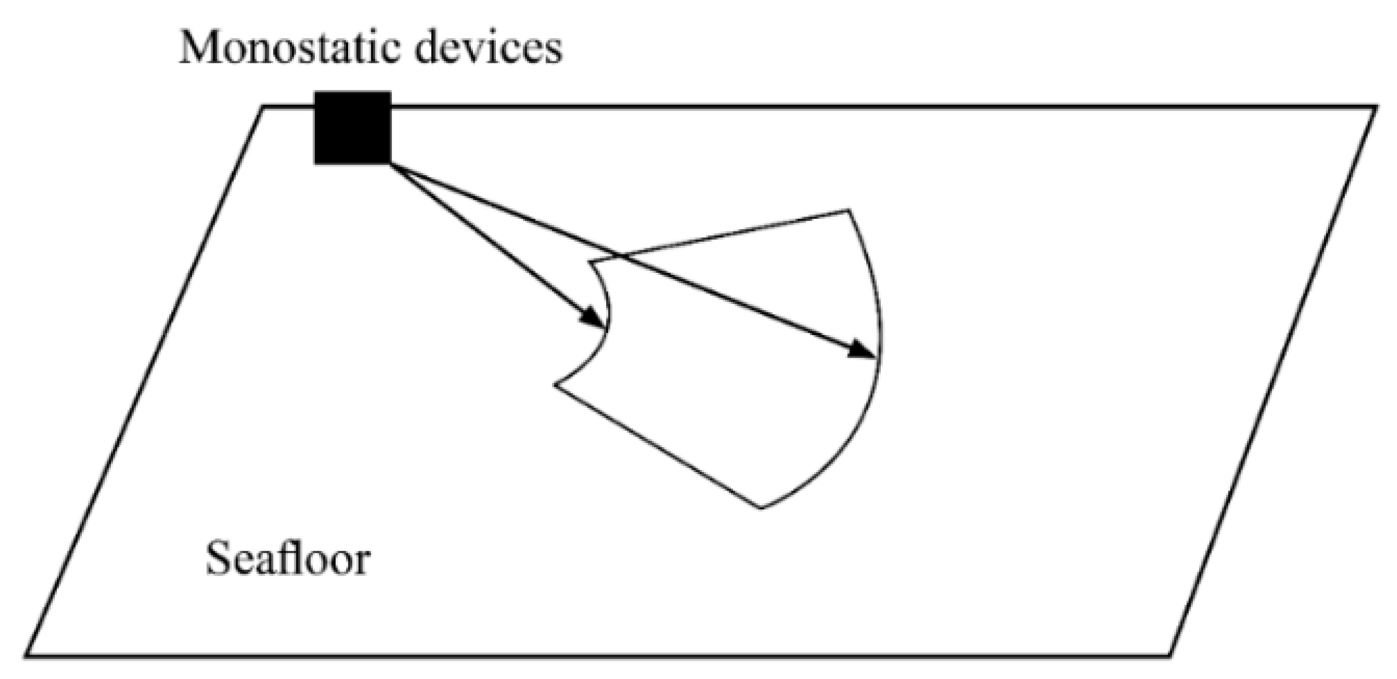
2.1. The Traditional Point-Scattering Method

Traditional seafloor reverberation simulation theory is generally based on two types of scattering models, namely the point-scattering model and the element-scattering model. Based on a statistical approach, the point-scattering model assumes that scatterers are randomly distributed throughout the ocean. The reverberation is calculated by summing the echoes of each individual scatterer. The point-scattering model is applicable to high-frequency sonar and subglacial scattering [7]. In this study, the point-scattering model is used for simulation as a comparison. As an example, the model of the monostatic devices is shown in Figure 1.

During a period T, the scattering area corresponding to the transmitted signal can be roughly viewed as a fan ring. This region of the fan ring is called the sampling element. The azimuth of the sampling element is limited by the beam pattern and the distance is limited by the period of the transmitted signal. The area of the sector ring can be calculated based on the speed of sound and the period of the wavelength. After calculating the area of the fan ring, the number of scatterers in the fan ring can be calculated based on the scatterer density. Based on the above information, the reverberant signal can be modeled as follows [36]:

$$R\left(t\right)=ℱ\left[{\displaystyle \sum }_{i=1}^{N\left(t\right)}S\left(r_i,{\phi }_i\right)f^2\left(d\left(r_i,{\phi }_i\right)\right)B_{TR}\left(r_i,{\phi }_i\right)x^{+}\left(t-\tau \left(r_i,{\phi }_i\right)\right)e^{j{\varphi }_i}\right]$$

(1)

where r_i is the distance coordinate, φ_i is the azimuth coordinate, (r_i,φ_i) is the coordinate vector of the ith scatterer, S is the scattering term, B_TR is the beam pattern of the monostatic sonar, f is the propagation term, d is the distance between the scatterer and the sonar, $\tau$ is the two-way propagation time delay, x⁺(t) is the analytic signal of the emitted signal x(t), and ${\varphi }_i$ is the random phase perturbation in the scattering process, uniformly distributed in [0, 2π].

Usually, S, f, and B_TR exhibit slow fluctuation characteristics relative to x⁺(t) in Equation (1). When the signal period T is small, x⁺(t) also exhibits slow fluctuation characteristics within the sampling element. In this case, the reverberation model can be expressed as [37]

$$R\left(t\right)\approx ℱ\left[{\displaystyle \sum }_{k=1}^{Ns}I\left(kT\right)x^{+}\left(t-kT\right)\right]$$

(2)

where I(kT) denotes the result of the common action of the scatterers about $S{f}^2{B}_{TR}{e}^{j\varphi }$ in the kth sampling element, which is calculated as follows:

$$I\left(kT\right)={\displaystyle \sum }_{i=1}^{N_a\left(kT\right)}S\left(r_i\right)f^2\left(d\left(r_i\right)\right)e^{j{\varphi }_i}$$

(3)

where N_a is the number of the scatterers in the sampling unit. In Equation (3), the scattering item S can be expressed as [37]

$$S=\sqrt{{10}^{\frac{\mu }{10}}sin\left({\alpha }_i\right)sin\left({\alpha }_o\right)}$$

(4)

where μ is vertical scattering coefficient, α_i is the incident grazing angle, and ${\alpha }_o$ is the scattering grazing angle. In the case of monostatic sonar, α_i is equal to ${\alpha }_o$. The propagation term f can be expressed as follows [38]:

$$f\left(d\right)=\frac{1}{d}{10}^{-\beta d}v$$

(5)

where β represents the absorption coefficient of seawater.

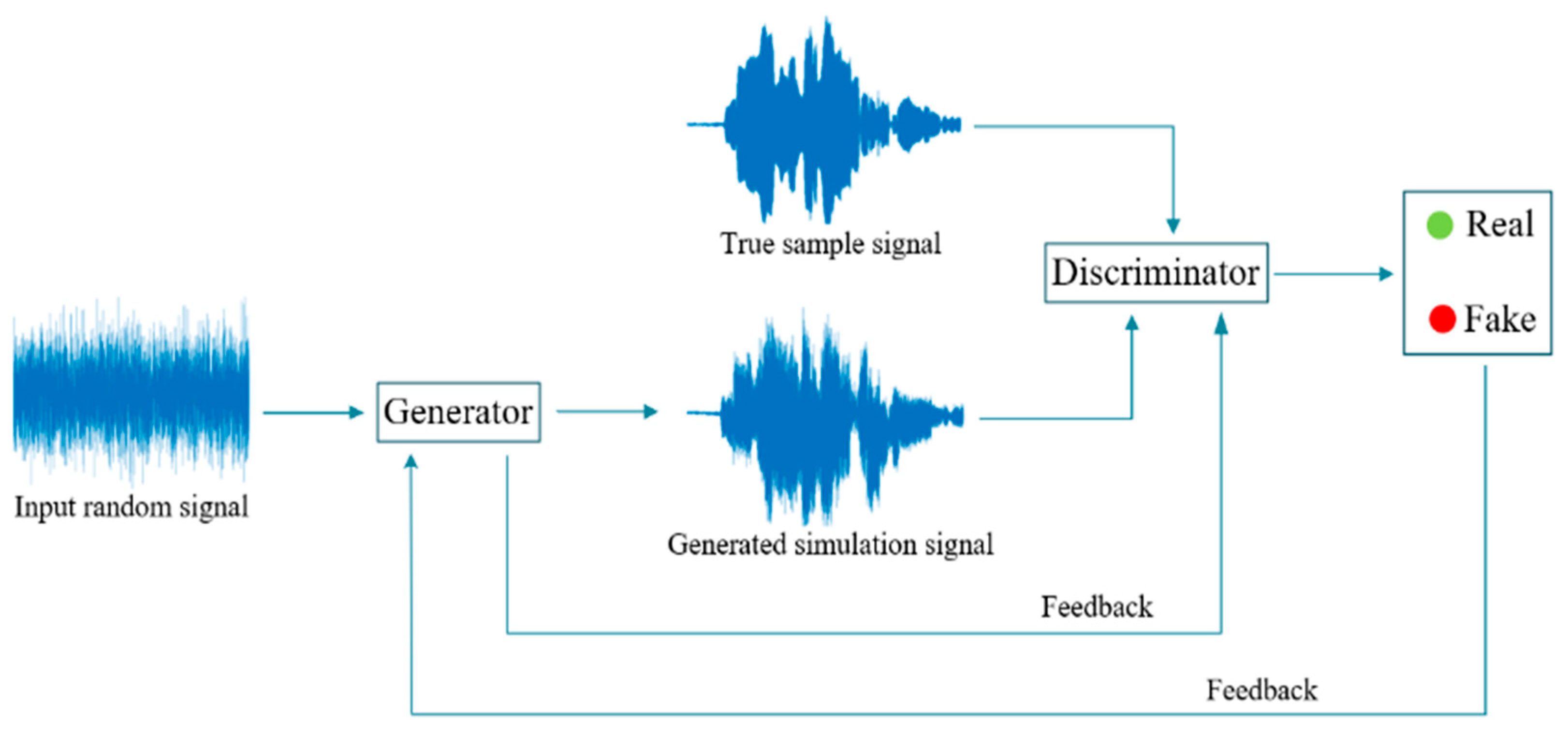
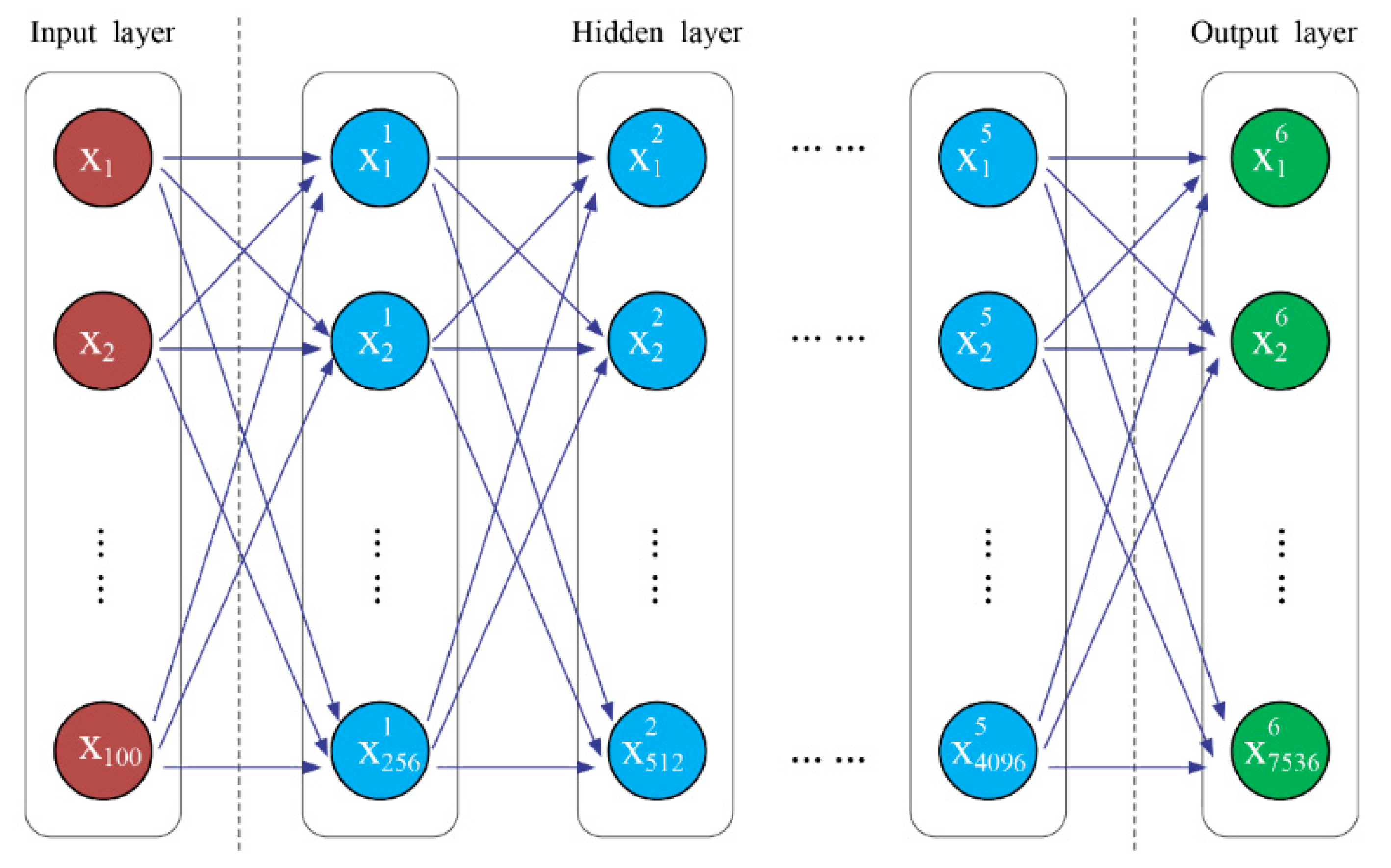
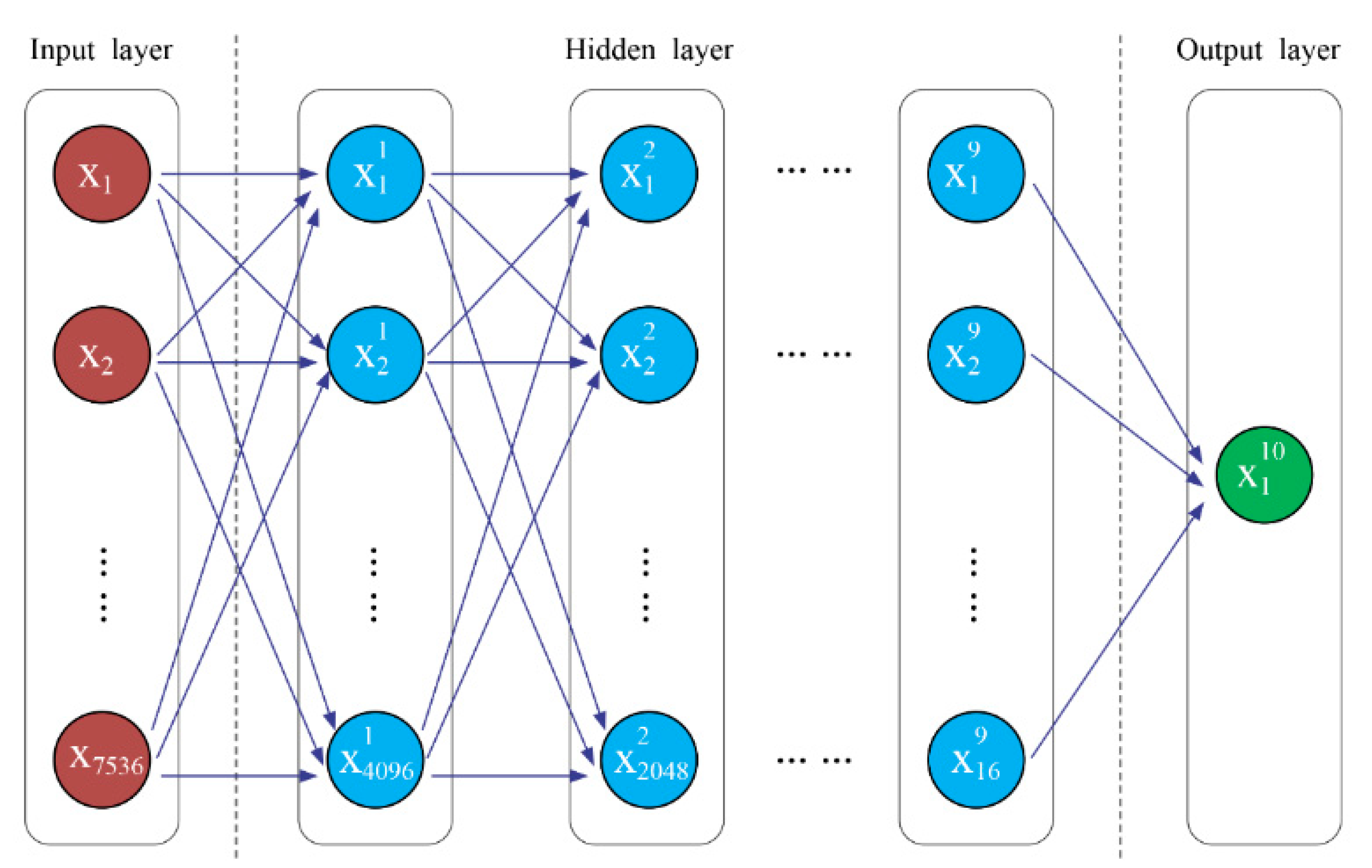
2.2. Generative Adversarial Network

2.2.1. The Strategy of the GAN

The goal of the GAN is to use the simulated data distribution $P_G\left(\mathit{x}\right)$ of the generator to match the actual sample data distribution $P_{data}\left(\mathit{x}\right)$. In this process, the GAN does not try to assign a deterministic probability to each $\mathit{x}$ of the data distribution but generates simulated data x by feeding the noisy variable $\mathit{z}~P_{noise}\left(\mathit{z}\right)$ into the generator $G\left(\mathit{z},{\mathit{\theta }}_{\mathit{g}}\right)$. The simulated data sample $\mathit{x}=G\left(\mathit{z},{\mathit{\theta }}_{\mathit{g}}\right)$ generated by the generator is fed into a discriminator $D\left(\mathit{x},{\mathit{\theta }}_{\mathit{d}}\right)$ to discriminate and output the discriminated results as right or wrong. The discriminator D and the generator G are both learnable neural networks. There is a mechanism of confrontation and mutual feedback between the two neural networks. Eventually, both the generator G and the discriminator D reach equilibrium at their respective high performance. However, the high performance of the generator G is achieved under the high-performance condition of the discriminator D. In this case, when the simulation data sample $\mathit{x}=G\left(\mathit{z},{\mathit{\theta }}_{\mathit{g}}\right)$ is passed to the discriminator G, the probability of discriminating as true or false is 1/2 each.

2.2.2. The Loss Function of the GAN

In the GAN, there exist two neural networks, the generator G and the discriminator D. The loss function should be built by considering both of them. Since the high performance of the generator G is achieved under the condition of high performance of the discriminator D, the loss function of the discriminator network D is considered first. The loss function [39] of the discriminator network D is as follows:

$$\underset{D}{\mathit{max}}\left\{E_{\mathit{x}~P_{data\left(\mathit{x}\right)}}\left[logD\left(\mathit{x}\right)\right]+E_{\mathit{z}~P_{noise\left(\mathit{z}\right)}}\left[log\left(1-D\left(G\left(\mathit{z}\right)\right)\right)\right]\right\}$$

(6)

For the generator network G, the loss function [39] is

$$\underset{G}{\mathit{min}}\left\{E_{\mathit{z}~P_{noise\left(\mathit{z}\right)}}\left[log\left(1-D\left(G\left(\mathit{z}\right)\right)\right)\right]\right\}$$

(7)

Considering Equations (6) and (7), the final loss function [40] is

$$\underset{G}{\mathit{min}}\underset{D}{\mathit{max}}\left\{E_{\mathit{x}~P_{data\left(\mathit{x}\right)}}\left[logD\left(\mathit{x}\right)\right]+E_{\mathit{z}~P_{noise\left(\mathit{z}\right)}}\left[log\left(1-D\left(G\left(\mathit{z}\right)\right)\right)\right]\right\}$$

(8)

2.2.3. The Training of the GAN

The whole GAN training process requires training both generator and discriminator neural networks. However, the discriminator performance is generally stronger than the generator at the beginning. Therefore, the whole training process is generally divided into two stages. The first stage trains the discriminator, and the second stage trains the generator. After training the discriminator, the discriminator passes true–false information to the generator. The generator receives the true–false information from the discriminator and continuously optimizes the network according to the information to generate high-quality samples.

The training of the GAN requires the calculation of the partial derivatives of the loss function with respect to ${\mathit{\theta }}_{\mathit{g}}$ and ${\mathit{\theta }}_{\mathit{d}}$. Detailed steps are as follows:

i. Input the actual sample data and the generator simulation data into the discriminator D for training and to update the parameters, and calculate the following equation [41]:

$${\nabla }_{{\theta }_d}\left\{E_{x~P_{data\left(x\right)}}\left[logD\left(x\right)\right]+E_{z~P_{noise\left(z\right)}}\left[log\left(1-D\left(G\left(z\right)\right)\right)\right]\right\}$$

(9)

The gradient ascent method is used to update ${\mathit{\theta }}_{\mathit{d}}$.

ii. Input the random-noise variable $\mathit{z}~P_{noise}\left(\mathit{z}\right)$ into the generator for training to update the parameters, and calculate the following equation [41]:

$${\nabla }_{{\mathit{\theta }}_{\mathit{g}}}\left\{E_{\mathit{z}~P_{noise\left(\mathit{z}\right)}}\left[log\left(1-D\left(G\left(\mathit{z}\right)\right)\right)\right]\right\}$$

(10)

The gradient descent method is used to update ${\mathit{\theta }}_{\mathit{g}}$.

iii. Repeat i, ii.

In this process, care should be taken to balance the capabilities of the generator and the discriminator so as not to cause one of them to be too powerful. Alternating updates of the generator and discriminator can be used to reach the global optimal solution. Through this learning strategy, the discriminator and generator continuously improve their abilities to discriminate and generate the adversarial.

2.3. The GAN Reverberation Simulation Method

In the adversarial network of this study, the random signal is input to the generator, and the generator is adjusted according to the information returned from the previous discriminator, so as to generate a new signal according to the input random signal. The signal generated by the generator is input into the discriminator together with the actual reverberation reference signal, and the discriminator judges whether the signal generated by the generator is true according to the actual reverberation reference signal. If true, the discriminator outputs 1, and if false, the discriminator outputs 0. The output information is fed back to the generator to enhance its ability of mixing the spurious with genuine. On the other hand, the discriminator optimizes and improves its performance based on the more realistic signals generated by the generator. In this way, the generator and the discriminator form an adversarial relationship, which makes the GAN reverberant signal simulation theoretically possible.

The framework of the GAN used in this paper is shown in Figure 2.

2.4. The Holistic Research Approach

In this study, we first input the environmental parameters of a sea area in China into the point-scattering model to generate the reverberation simulation data. Then, the actual sea trial reverberation data of the same sea area are input into the GAN to generate the reverberation simulation data. Finally, the statistical characteristics of the reverberation simulation data generated by the two methods are compared and analyzed to determine whether the GAN reverberation generation method is feasible. The holistic research flow chart is shown in Figure 3 below.

3. Simulation

3.1. The Simulation Based on the Point-Scattering Method

In this section, the point-scattering model was used for the reverberation simulation. The continuous wave (CW) signal and the linear frequency modulation (LFM) signal were simulated separately, and the parameters of the point-scattering model are shown in

Table 1. The parameters of the point-scattering model.

Parameter	CW	LFM
Center frequency (HZ)	500	500
Sampling frequency (HZ)	5000	5000
Bandwidth (HZ)	-	200
Beam angle (°)	30	30
Vertical scattering coefficient (dB)	−27	−27
Seawater absorption coefficient	0	0
Scatterer density	20	20
Sound speed (m/s)	1500	1500
Start time (s)	0.08	0.08
End time (s)	0.23	0.23
Pulse width (s)	0.05	0.05
Launch duration time (s)	0.5	0.5
Distance between the device and the seabed (m)	50	50

.

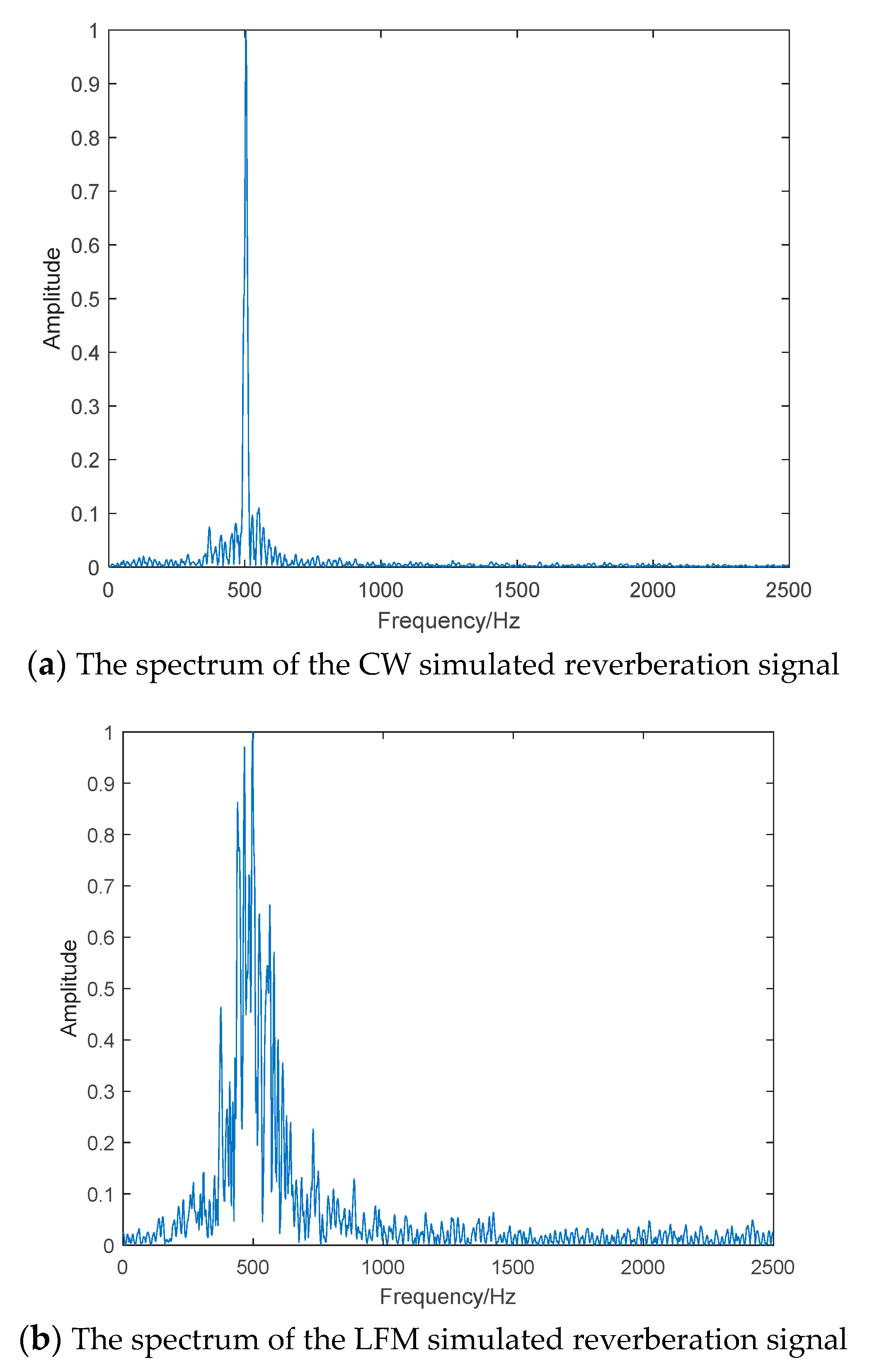
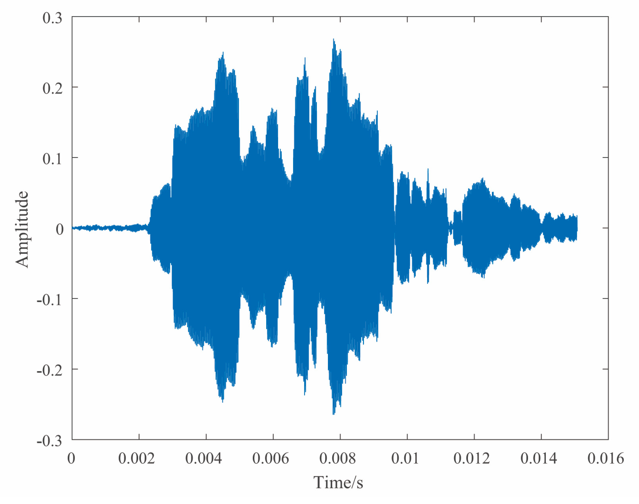
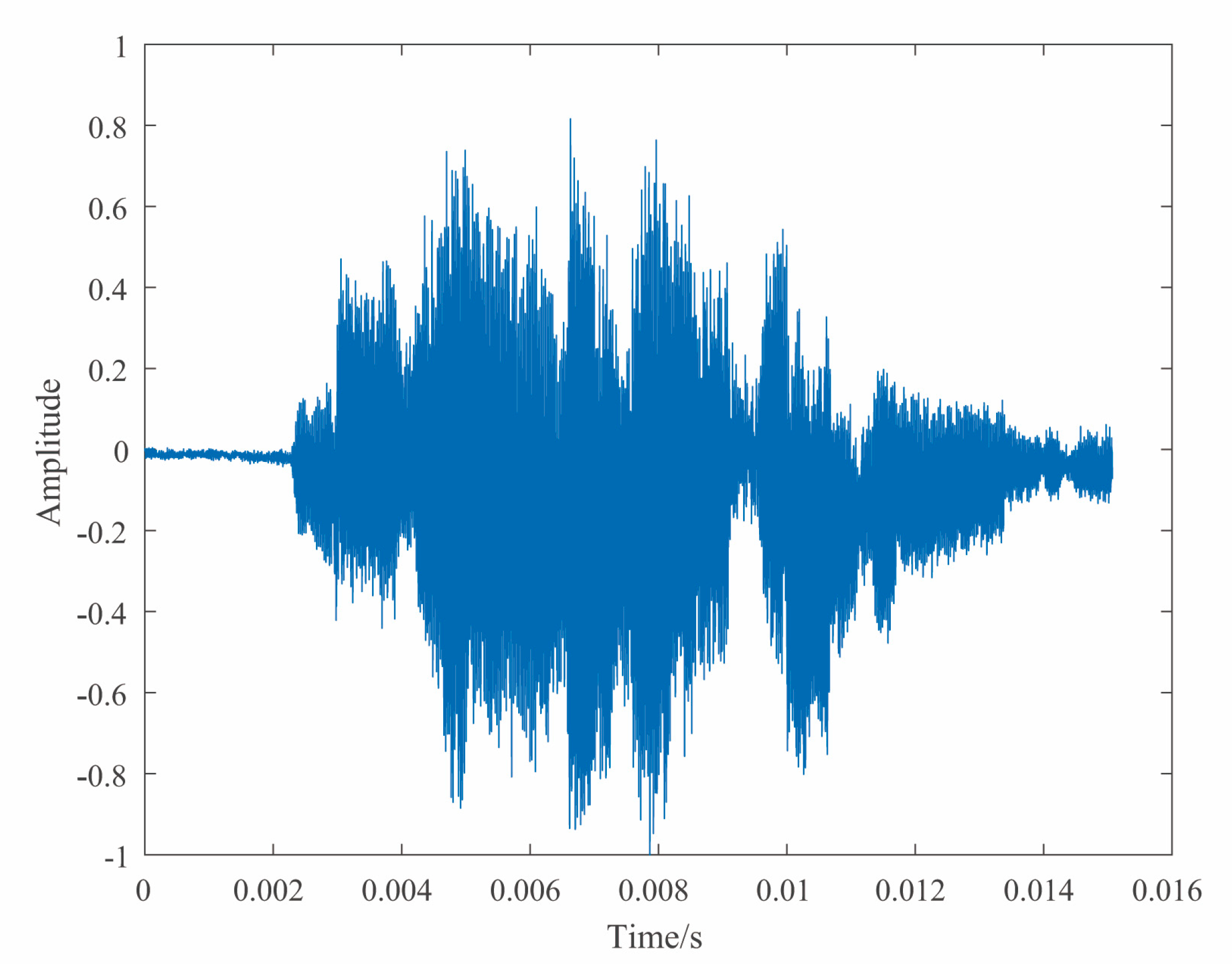
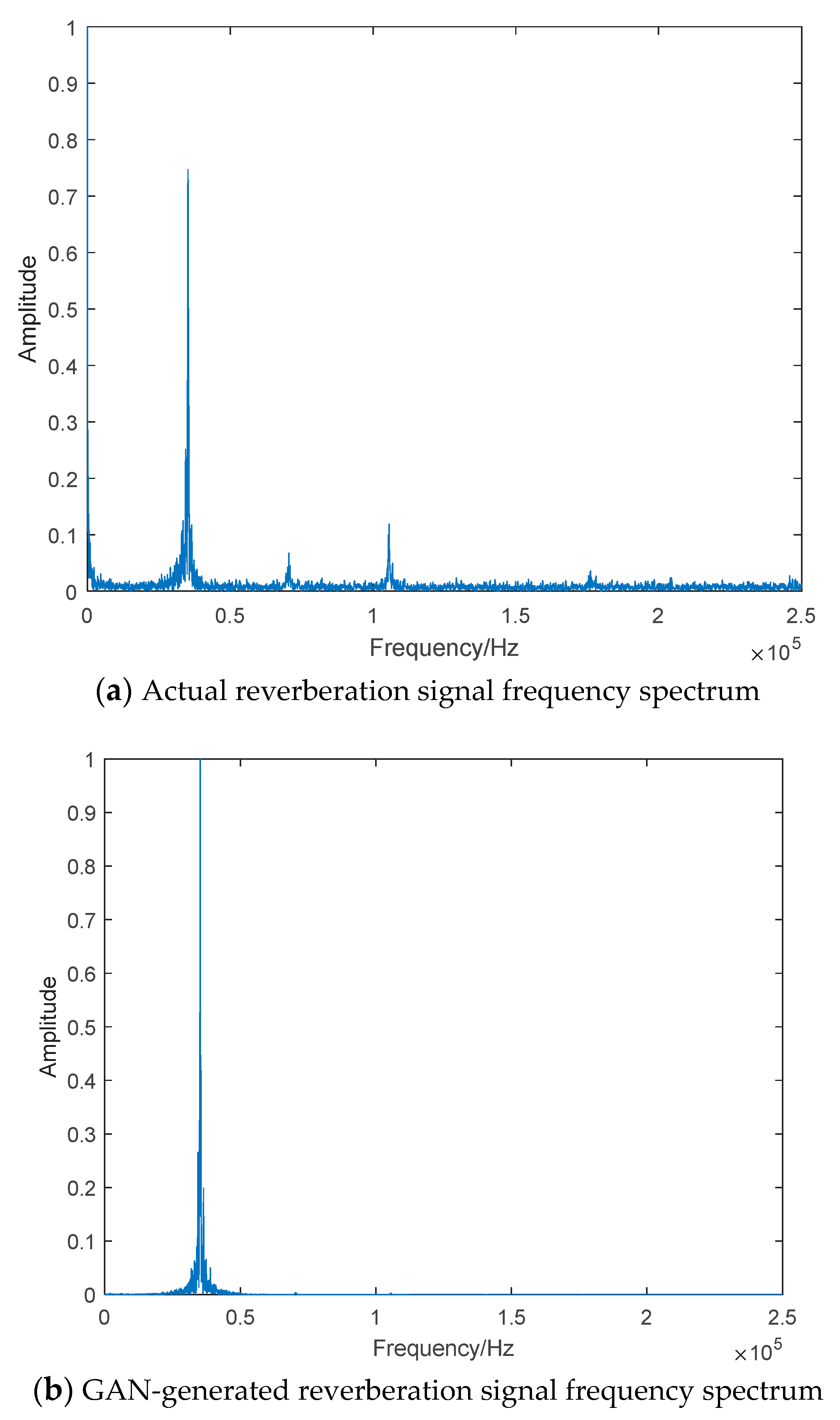
3.1.1. Time–Frequency Characteristics of the Reverberation Signal

It can be seen from Figure 4 that the reverberation data are in the interval of 0.08 s–0.23 s. In the time domain, the amplitude of the signal scattered back by the scattering element is random, with large fluctuations. The envelope of the reverberation signal decays with time according to certain rules, which is a nonstationary random process that shows the nature of reverberation.

The following is the time domain waveform of the simulated reverberation signal.

Fourier transform was performed on the reverberation signal. Figure 5 shows the CW and LFM reverberation spectra, respectively. According to the above theory, the frequency domain of the reverberation signal is similar to that of the transmitted signal. Observing the amplitudes in Figure 5, it can be seen that the center frequencies of both the CW and LFM reverberation signals are 500 Hz, and the bandwidth of LFM reverberation signal is close to 200 Hz, which indicates that the simulation results of the point-scattering model satisfy the reverberation characteristics.

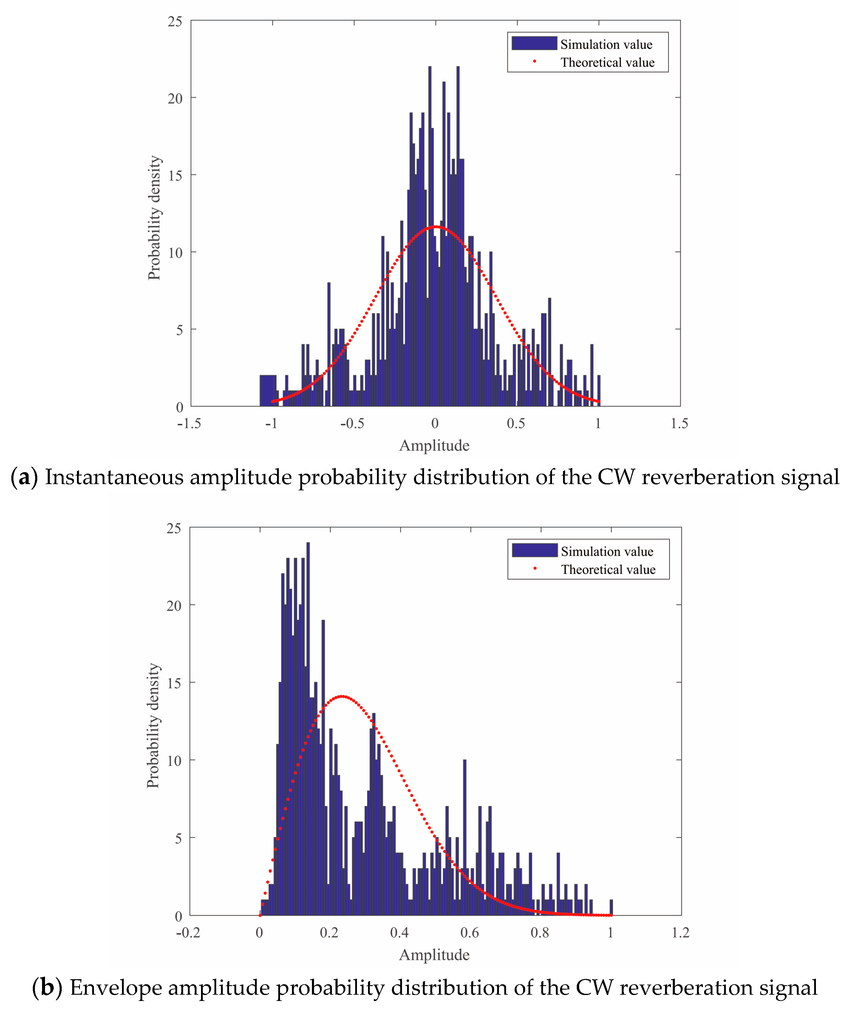
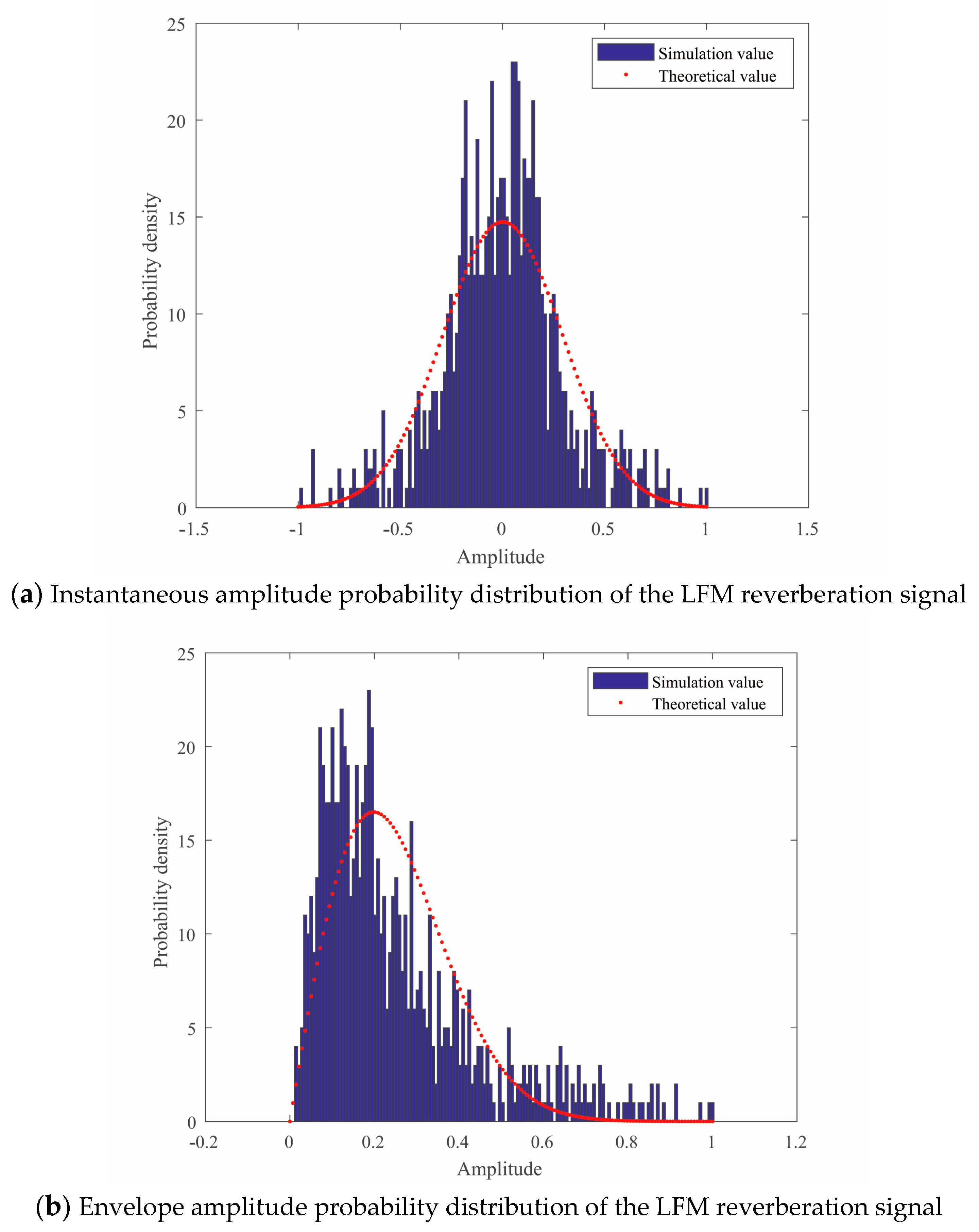
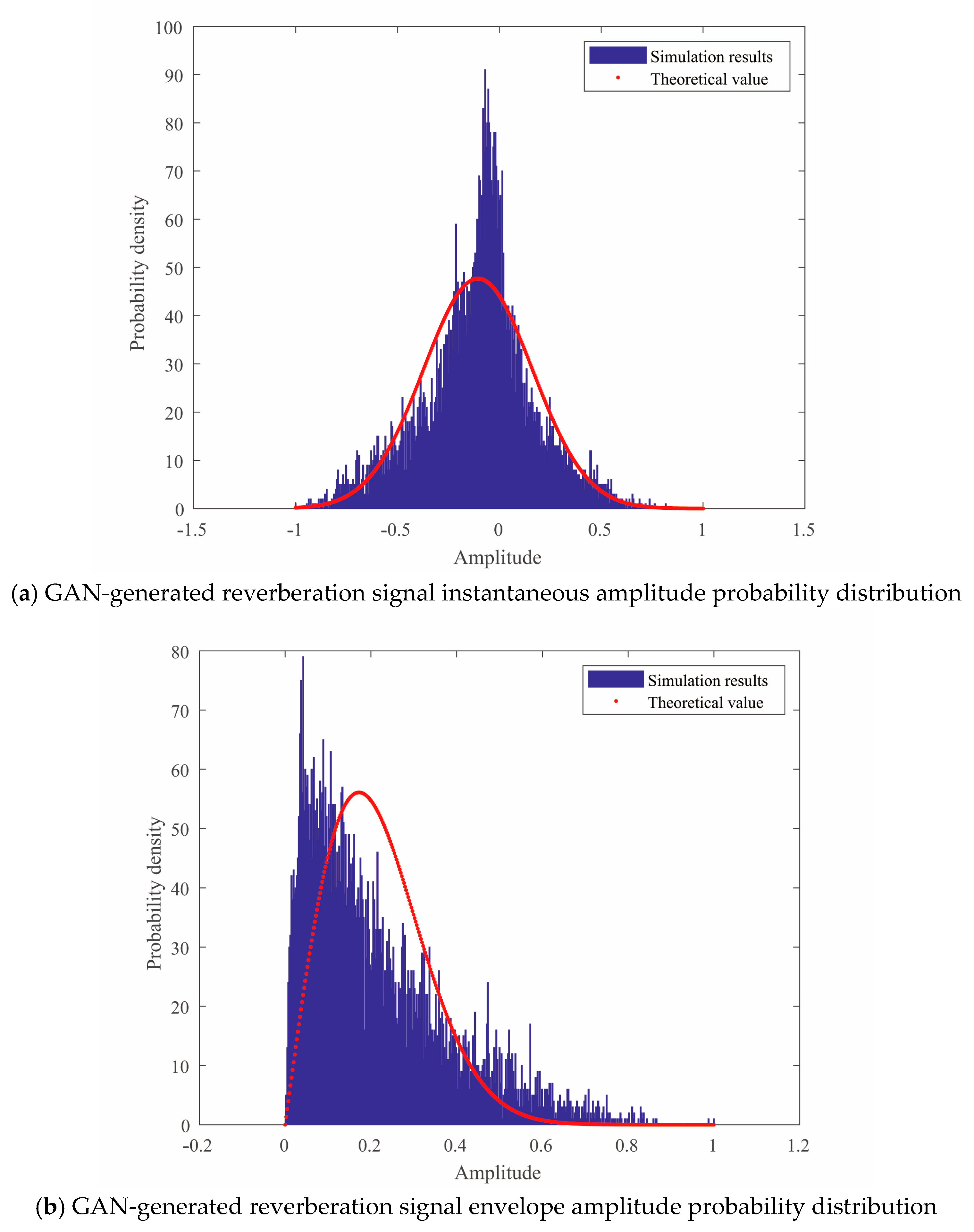
3.1.2. Statistical Characteristics of the Reverberation Simulation

If the transmit signal is narrowband, it is known from the central limit theorem and random signal analysis theory that the instantaneous value of the reverberation signal obeys the Gaussian distribution, and the envelope of the reverberation signal obeys the Rayleigh distribution. The reverberation instantaneous value V(t) satisfies the Gaussian distribution with a probability density function [42] of

$$W\left(V\right)=\frac{1}{\sqrt{2\pi {\sigma }_V}}\exp \left(-\frac{V^2}{2{\sigma }_V^2}\right)$$

(11)

In Equation (11), W is the probability density and ${\sigma }_V^2$ is the instantaneous value variance of the reverberation signal.

The envelope E(t) of the reverberant signal satisfies the Rayleigh distribution with a probability density function [43] of

$$W\left(E\right)=\frac{1}{{\sigma }_V^2}\exp \left(-\frac{E^2}{2{\sigma }_V^2}\right)$$

(12)

In Equation (12), W is the probability density and ${\sigma }_V^2$ is the instantaneous value variance of the reverberation signal.

According to the above parameters, the statistical characteristics of the reverberation signal are obtained and are shown in Figure 6.

Figure 6a and Figure 7a plot the instantaneous value probability distributions. Figure 6b and Figure 7b plot the envelope probability distributions. The purple bars show the probability distributions of the simulated signal, and the red dots show the theoretical values of the associated distributions. From the figures, it can be seen that the instantaneous amplitude distribution obtained with the point-scattering model is close to the Gaussian distribution, and the envelope amplitude distribution is close to the Rayleigh distribution, which satisfy the theoretical reverberation characteristics.

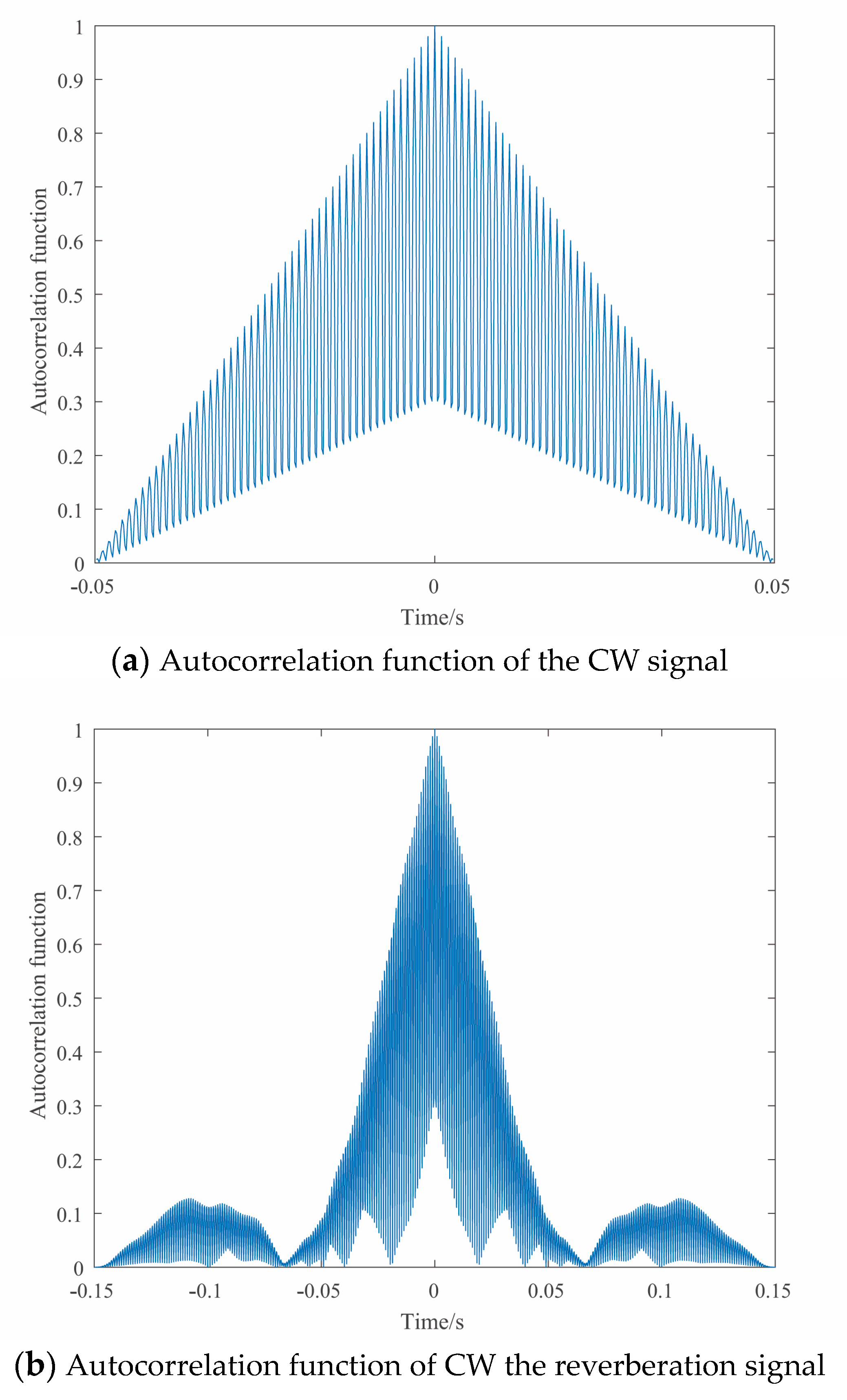
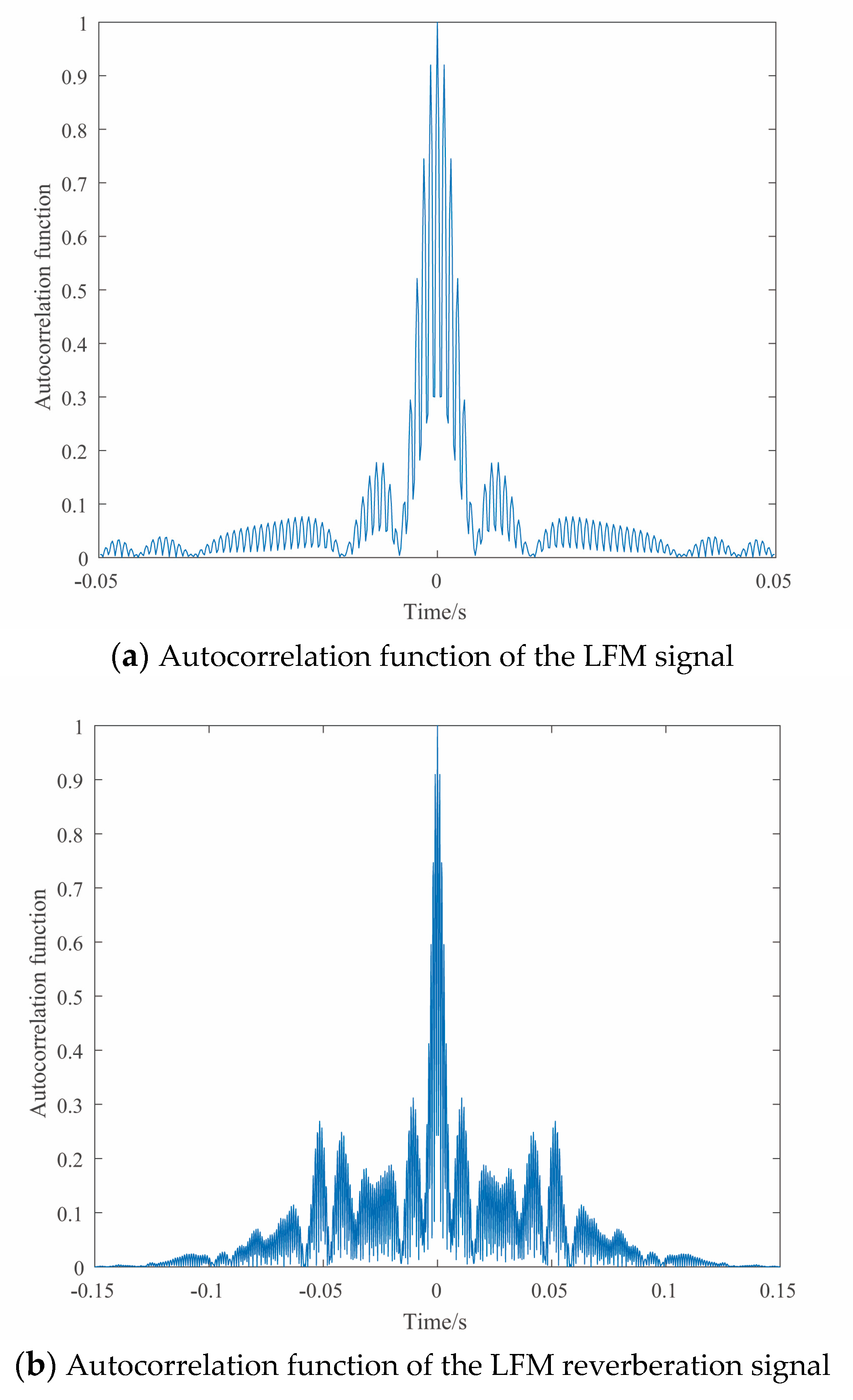
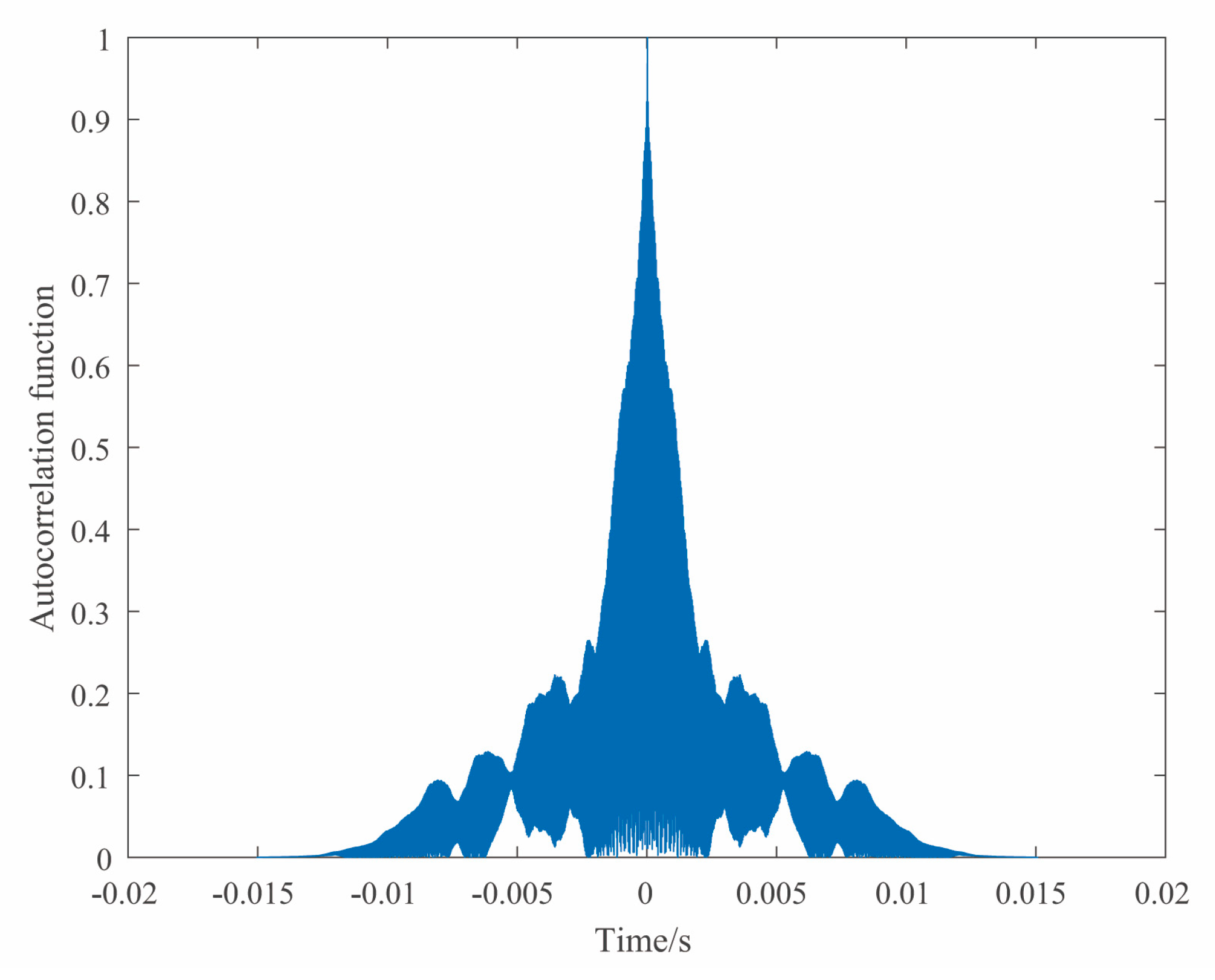
3.1.3. Time Domain Correlation Characteristics of the Reverberation Simulation

Although the statistical characteristics of the reverberation signal depend on time, it can still be considered as a stationary random process locally or in a short time. Since the time-varying characteristics of the signal is much slower than itself, some random process analysis can still be used here.

The time dependence of a reverberation signal is described by the autocorrelation function, if a reverberation signal is

$$s\left(t\right)=s_0\left(t\right)cos\left[{\omega }_0\left(t\right)+\mathit{\Phi }\left(t\right)\right]$$

(13)

then the autocorrelation function [44] is

$$R\left(\tau \right)\approx \frac{1}{\delta }\left\{{{\displaystyle \int }}_{-\infty }^{\infty }{s}_0\left(t\right)s_0\left(t+\tau \right)cos\left[\mathit{\Phi }\left(t+\tau \right)-\mathit{\Phi }\left(t\right)\right]dt\right\}cos{\omega }_0\tau$$

(14)

After a little analysis of the above equation, it can be seen that the autocorrelation function of a reverberation signal is similar to that of its transmitted signal, and its autocorrelation function decays with the time. The duration of a reverberation signal is much longer than that of the transmitted pulse width. It has relevant characteristics similar to that of the transmitted signal within the duration. With the increase in duration, the amplitude gradually decreases. When the time correlation is close to zero, it means that the reverberation signal is basically over.

Figure 8a shows the autocorrelation function of the CW signal, and Figure 8b shows the autocorrelation function of the CW reverberation signal. Comparing the two figures, we can find that the autocorrelation function of reverberation and signal is similar. The autocorrelation function is the largest in the middle moment, and the middle moment corresponds to the moment of 0. After that, the amplitude gradually decreases with the increase in time, and finally tends to 0, which is consistent with the theoretical analysis. Figure 9 is similar to Figure 8.

In this study, the time domain correlation characteristics of the reverberation signal are described by its autocorrelation function. The time domain correlation functions of the CW signal, the CW reverberation signal, the LFM signal, and the CW reverberation signal are plotted as follows.

From a theoretical point of view, the calculation amount of the point-scattering model is influenced by the period of the emitted signal, the density of the ocean scatterer, and the sampling frequency. The area of the scattering element in the reverberant zone is first determined according to the emission signal period, then the number of sampling points in its next period is determined according to the sampling frequency. Finally, the calculation amount of each sampling point is determined according to the density of the scatterer. In the calculation process, when any one of the above three factors is amplified, the overall calculation cost tends to increase by hundreds or thousands of times. In this case, it is necessary to wait a long time for each reverberation simulation. In addition, the nonuniversality of some parameters in the scattering model, for example, the scatterer density which changes with the specific sea area, leads to a reduction in the generalizability of the reverberation model.

3.2. The Simulation Based the GAN

In this section, the GAN is used for the reverberation simulation, and the actual reverberation data from the sea trials in shallow water in China are used as the actual reference reverberation signals for training. The emission signals of the sea trial reverberation data are CW signals with a center frequency of 35 kHz, a sampling frequency of 500 kHz and a pulse width of 2 ms. Its time domain waveform is shown in Figure 10.

The generator uses a seven-layer neural network, including an input layer, five hidden layers and an output layer. The input of the whole generative network is a random vector with a length of 100, and the output is the reverberation data with a length of 7536 after the processing of the five-layer network. The number of nodes in the first hidden layer is 256, and the activation function is the Leaky ReLU function. The input layer is fully connected to the first hidden layer. The number of nodes in the remaining hidden layers are 512, 1024, 2048 and 4096, and the activation functions are all Leaky ReLU functions. All connections between hidden layers are fully connected. The number of nodes in the output layer network is 7536, and the activation function is the sigmoid function. The connection between the last hidden layer and the output layer is fully connected. The detailed structure is shown in Figure 11.

The input of the discriminator network is the reverberation data generated by the generator network with a length of 7536, and the output is 1 or 0 after processing in the hidden layers. An output of 1 means that the discriminator network judges the data to be true, and 0 means that the discriminator network judges the data to be false. The discriminator uses an eleven-layer neural network, including an input layer, nine hidden layers and an output layer. The number of nodes in the input layer is 7536, and the number of nodes in the first hidden layer is 4096. The activation function is the Leaky ReLU function, and the input layer is fully connected to the hidden first layer. The number of nodes in the remaining hidden layers are 2048, 1024, 512, 256, 128, 64, 32 and 16 nodes, and the functions are all Leaky ReLU functions. All connections between hidden layers are fully connected. The output length of the output layer is 1, and the activation function is the sigmoid function. The connection between the hidden last layer and the output layer is fully connected. The detailed structure is shown in Figure 12.

More than 1800 sets of actual sea trial data were used for this training. An Adam optimizer was used for optimization. The learning rate was 2 × 10⁻⁴. The training loss values are shown in Figure 13.

It can be seen from Figure 13 that the loss values of both networks converge, which means better training. The output reverberation signal using the trained GAN network is shown in Figure 14.

Next, the GAN-generated reverberation was analyzed for the reverberation characteristics to determine if it satisfies the reverberation characteristics. From Figure 14, it can be seen that the reverberation data are in the interval after 2 ms, and in the time domain, the envelope of the reverberation signal decays with time according to a certain law, which is a nonstationary random process that shows the nature of reverberation.

Fourier transform was performed on the GAN-generated reverberation signal. The frequency spectrum of the GAN-generated reverberation signal was compared with that of the actual sea trial data. The comparison results are shown in Figure 15. Figure 15a shows the frequency spectrum of the actual reverberation signal, and Figure 15b shows the frequency spectrum of the GAN-generated reverberation signal. From the figures, it can be seen that the frequency spectrum of the GAN-generated reverberation signal is similar to that of the actual reverberation signal, which is close to the frequency spectrum of the emitted signal. The highest point of the spectrum is at 35 kHz, which is consistent with the characteristics of the reverberation spectrum.

The statistical characteristics of the GAN-generated reverberation signal are shown in Figure 16.

As can be seen in Figure 16, the instantaneous amplitude distribution of the GAN-generated reverberation signal is close to the Gaussian distribution, and the envelope distribution is close to the Rayleigh distribution, which satisfy the theoretical reverberation characteristics.

According to the theory above, the autocorrelation function of reverberation is similar to that of a transmitted signal, and its autocorrelation function decays with time. The duration of a reverberation signal is much longer than that of the transmitted pulse width. It has relevant characteristics similar to that of the transmitted signal within the duration. With the increase in duration, the amplitude gradually decreases. When the time correlation is close to zero, it means that the reverberation signal is basically over. The GAN-generated reverberation signal is consistent with this theory, as seen in Figure 17.

The following is a plot of the time domain correlation function of the GAN-generated reverberation signal:

4. Conclusions

This paper first introduces the importance of a reverberation characteristic study for the implementation of the reverberation suppression algorithms and presents one of the difficulties that needs to be overcome before the reverberation characteristic study: the acquisition of the reverberation signals. To address this difficulty, a reverberation simulation method based on the GAN is proposed for efficient reverberation signal study. First, the reverberation signal is simulated based on the traditional point-scattering model, and the reverberation characteristics are analyzed and summarized in various aspects. Then, the reverberation signal is simulated based on the GAN, and the reverberation characteristics of the simulated signal are also analyzed and summarized. The reverberation characteristics are also compared with those of the simulation signal obtained by the conventional point-scattering model.

By comparing Figure 3 and Figure 9, it can be seen that the reverberation simulation data based on the GAN have the same characteristics in the time domain as the reverberation simulation data obtained from the traditional point-scattering model, and they are all consistent with the time domain characteristics of the reverberation. By comparing Figure 4 and Figure 14, it can be seen that the reverberation simulation data based on the GAN are similar to the reverberation simulation data obtained from the traditional point-scattering model in the frequency domain. The center frequencies are all 500 Hz, which satisfies the reverberation characteristics. By comparing Figure 5, Figure 6 and Figure 15, it can be seen that the reverberation simulation data based on the GAN and the traditional point-scattering model are both close to the Gaussian distribution in the instantaneous amplitude distribution and close to the Rayleigh distribution in the envelope distribution, which satisfy the reverberation characteristics. By comparing Figure 7, Figure 8 and Figure 16, it can be seen that the reverberation simulation data based on the GAN and the traditional point-scattering model are similar in terms of correlation, and they both gradually weaken with time, which satisfy the reverberation characteristics. Therefore, it is theoretically feasible to use the GAN to generate reverberant signals.

In terms of calculation cost, the main factors affecting the calculation cost of the point-scattering model are the emission signal period, ocean scatterer density, sampling frequency, etc. When any one of the above three factors is amplified, the overall calculation cost is often increased hundreds or thousands of times, so it is necessary to wait a long time for each reverberation simulation. Unlike the point-scattering model, the GAN-based reverberation simulation method requires a high computational effort only when the network is trained. Once the network is trained, the computational effort for each subsequent reverberation generation is negligible. Therefore, in comparison, the GAN-based reverberation simulation method is less computationally intensive.

In terms of universality, the reverberation simulation method based on the point-scattering model is theoretically fixed and the parameters, such as the emission signal and the scatterer density, can only be slightly modified according to the different test conditions. However, the proposed GAN-based reverberation simulation method is different. As long as there is a small amount of the actual reverberation signal of the sea, the GAN can use these signals as samples to simulate the reverberation signals with a high degree of similarity. Therefore, in comparison, the proposed GAN-based reverberation simulation method has higher universality.

From the above analysis, it is concluded that the reverberation simulation data based on the GAN are similar to those based on the traditional point-scattering model in terms of the time and frequency domains, statistical characteristics and correlation characteristics, and they can be better applied to the subsequent study of reverberation suppression schemes. However, the proposed GAN-based reverberation simulation method has more obvious advantages in terms of calculation cost and universality. Of course, there are shortcomings in the method proposed in this paper. More data from a few sea areas should be used to verify the generalizability of the proposed method, as well as to explore the influences of network structure and type on the simulation results, etc.

References

1. Kun, X.; Wang, Q.Y. Blind Separability of Reverberation and Target Echo Based on Spatial Correlation. Appl. Mech. Mater. 2011, 128–129, 538–543. [Google Scholar]
2. Li, P.; Qiu, H.; Wang, C.; Wu, Y.; Miao, F. Research on Reverberation Cancellation Algorithm Based on Empirical Mode Decomposition. In Proceedings of the 2020 IEEE International Conference on Information Technology, Big Data and Artificial Intelligence, Chongqing, China, 6–8 November 2020. [Google Scholar]
3. Shang, E.C.; Gao, T.; Wu, J. A Shallow-Water Reverberation Model Based on Perturbation Theory. IEEE J. Ocean. Eng. 2008, 33, 451–461. [Google Scholar] [CrossRef]
4. Katsnelson, B.; Petnikov, V.; Lynch, J. Low-Frequency Bottom Reverberation in Shallow Water. In Fundamentals of Shallow Water Acoustics; Springer: New York, NY, USA, 2012; pp. 239–266. [Google Scholar]
5. Badeau, R. Unified Stochastic Reverberation Modeling. In Proceedings of the 2018 26th European Signal Processing Conference (EUSIPCO), Rome, Italy, 3–7 September 2018; pp. 2175–2179. [Google Scholar]
6. Etter, P.C. Underwater Acoustic Modeling and Simulation; CRC Press: Boca Raton, FL, USA, 2018. [Google Scholar]
7. Lee, K.; Chu, Y.; Seong, W. Geometrical Ray-Bundle Reverberation Modeling. J. Comput. Acoust. 2013, 21, 1350011. [Google Scholar] [CrossRef]
8. Bucker, H.P.; Morris, H.E. Normal-Mode Reverberation in Channels or Ducts. J. Acoust. Soc. Am. 1968, 44, 827–828. [Google Scholar] [CrossRef]
9. Bjørnø, L.; Neighbors, T.; Bradley, D. Applied Underwater Acoustics; Elsevier: Amsterdam, The Netherlands, 2017. [Google Scholar]
10. Ellis, D.D.; Yang, J.; Preston, J.R.; Pecknold, S. A Normal Mode Reverberation and Target Echo Model to Interpret Towed Array Data in the Target and Reverberation Experiments. IEEE J. Ocean. Eng. 2017, 42, 344–361. [Google Scholar] [CrossRef]
11. Collis, J.M.; Frank, S.D.; Metzler, A.M.; Preston, K.S. Elastic Parabolic Equation and Normal Mode Solutions for Seismo-Acoustic Propagation in Underwater Environments with Ice Covers. J Acoust Soc Am 2016, 139, 2672. [Google Scholar] [CrossRef]
12. Hefner, B.T.; Hodgkiss, W. Reverberation Due to a Moving, Narrowband Source in an Ocean Waveguide. J. Acoust. Soc. Am. 2019, 146, 1661–1670. [Google Scholar] [CrossRef]
13. Zuo, Y.; Gao, B.; Song, W.; Pang, J.; Mo, D. A Coupled Mode Method for Low Frequency Distant Reverberation in Deep Water Environment with Ice Covers. In Proceedings of the 2021 OES China Ocean Acoustics (COA), Harbin, China, 14–17 July 2021. [Google Scholar]
14. Pang, J.; Gao, B.; Song, W.; Zuo, Y.; Mo, D. A Coupled Mode Reverberation Theory for Clutter Induced by Inhomogeneous Water Columns in Shallow Sea. In Proceedings of the 2021 OES China Ocean Acoustics (COA), Harbin, China, 14–17 July 2021; pp. 526–529. [Google Scholar]
15. Tang, D.; Hefner, B.; Jackson, D. Direct-Path Backscatter Measurements Along the Main Reverberation Track of Trex13. IEEE J. Ocean. Eng. 2019, 44, 972–983. [Google Scholar] [CrossRef]
16. Li, N.; Zhang, M.; Gao, B. Horizontal Correlation of Long-Range Bottom Reverberation in Shallow Sloping Seabed. J. Mar. Sci. Eng. 2021, 9, 414. [Google Scholar] [CrossRef]
17. Guigné, J.Y.; Blondel, P. Acoustic Investigation of Complex Seabeds; Springer: Berlin/Heidelberg, Germany, 2017. [Google Scholar]
18. Zhou, J.X.; Zhang, X.Z. Integrating the Energy Flux Method for Reverberation with Physics-Based Seabed Scattering Models: Modeling and Inversion. J. Acoust. Soc. Am. 2013, 134, 55–66. [Google Scholar] [CrossRef]
19. Gao, B.; Wang, N.; Wang, H.Z. Investigation of Sea Surface Effect on Shallow Water Reverberation by Coupled Mode Method. J. Comput. Acoust. 2017, 25, 1750017. [Google Scholar] [CrossRef]
20. Wu, X.; Liu, J.; Zhang, C. Research and Analysis on the Reverberation Scattering Characteristics for Active Sonar Echo Detection System. RISTI Rev. Iber. Sist. E Tecnol. Inf. 2016, E6, 197–209. [Google Scholar]
21. Preuss, S.; Gurbuz, C.; Jelich, C.; Baydoun, S.K.; Marburg, S. Recent Advances in Acoustic Boundary Element Methods. J. Theor. Comput. Acoust. 2022, 30, 2240002. [Google Scholar] [CrossRef]
22. Makris, N.C.; Ratilal, P. A Unified Model for Reverberation and Submerged Object Scattering in a Stratified Ocean Waveguide. J. Acoust. Soc. Am. 2001, 109, 909–941. [Google Scholar] [CrossRef] [PubMed] [Green Version]
23. Ivakin, A.N. Sound Scattering by Random Inhomogeneities of Stratified Ocean Sediments. Sov. Phys. Acoust.-USSR 1986, 32, 492–496. [Google Scholar]
24. Ivakin, A.N. A Unified Approach to Volume and Roughness Scattering. J. Acoust. Soc. Am. 1998, 103, 827–837. [Google Scholar] [CrossRef]
25. Mourad, P.D.; Jackson, D. A Model/Data Comparison for Low-Frequency Bottom Backscatter. J. Acoust. Soc. Am. 1993, 94, 344–358. [Google Scholar] [CrossRef]
26. Galinde, A.; Donabed, N.; Andrews, M.; Lee, S.; Makris, N.; Ratilal, P. Range-Dependent Waveguide Scattering Model Calibrated for Bottom Reverberation in a Continental Shelf Environment. J. Acoust. Soc. Am. 2008, 123, 1270–1281. [Google Scholar] [CrossRef] [Green Version]
27. Goodfellow, I.; Pouget-Abadie, J.; Mirza, M.; Xu, B.; Warde-Farley, D.; Ozair, S.; Courville, A.; Bengio, Y. Generative Adversarial Networks. Commun. ACM 2020, 63, 139–144. [Google Scholar] [CrossRef]
28. Chan, E.R.; Monteiro, M.; Kellnhofer, P.; Wu, J.; Wetzstein, G. Pi-Gan: Periodic Implicit Generative Adversarial Networks for 3d-Aware Image Synthesis. In Proceedings of the IEEE/CVF Conference on Computer Vision and Pattern Recognition, Nashville, TN, USA, 20–15 June 2021. [Google Scholar]
29. Hudson, D.A.; Zitnick, L. Generative Adversarial Transformers. In Proceedings of the International Conference on Machine Learning, Virtual, 18–24 July 2021. [Google Scholar]
30. Shen, Y.; Zhou, B. Closed-Form Factorization of Latent Semantics in Gans. In Proceedings of the IEEE/CVF Conference on Computer Vision and Pattern Recognition, Nashville, TN, USA, 20–15 June 2021. [Google Scholar]
31. Wang, X.; Yu, K.; Wu, S.; Gu, J.; Liu, Y.; Dong, C.; Qiao, Y.; Loy, C.C. Esrgan: Enhanced Super-Resolution Generative Adversarial Networks. In Proceedings of the European Conference on Computer Vision (ECCV) Workshops, Munich, Germany, 8–14 September 2018. [Google Scholar]
32. Zhan, F.; Zhu, H.; Lu, S. Spatial Fusion Gan for Image Synthesis. In Proceedings of the IEEE/CVF Conference on Computer Vision and Pattern Recognition, Long Beach, CA, USA, 15–20 June 2019. [Google Scholar]
33. Dong, H.-W.; Yang, Y.-H. Convolutional Generative Adversarial Networks with Binary Neurons for Polyphonic Music Generation. arXiv 2018, arXiv:1804.09399. [Google Scholar]
34. Kumar, K.; Kumar, R.; de Boissiere, T.; Gestin, L.; Teoh, W.Z.; Sotelo, J.; de Brébisson, A.; Bengio, Y.; Courville, A. Melgan: Generative Adversarial Networks for Conditional Waveform Synthesis. In Proceedings of the Advances in neural information processing systems, Vancouver, BC, Canada, 8–14 December 2019; Volume 32. [Google Scholar]
35. Ratnarajah, A.; Tang, Z.; Manocha, D. Ir-Gan: Room Impulse Response Generator for Far-Field Speech Recognition. arXiv 2020, arXiv:2010.13219. [Google Scholar]
36. Abraham, D.A.; Lyons, A. Simulation of Non-Rayleigh Reverberation and Clutter. IEEE J. Ocean. Eng. 2004, 29, 347–362. [Google Scholar] [CrossRef]
37. Guo, X.-Y.; Su, S.-J.; Wang, Y.-K.; Chen, J.-Y. Research on Simulating Seafloor Reverberation in the Case of Monostatic. J. Natl. Univ. Def. Technol. 2010, 32, 141–145. [Google Scholar]
38. Ivakin, A.; Williams, K. Mid-Frequency Propagation and Reverberation in a Deep Ice-Covered Ocean: Modeling and Data Analysis. Proc. Meet. Acoust. 2020, 42, 070004. [Google Scholar]
39. Xia, K.; Yin, H.; Qian, P.; Jiang, Y.; Wang, S. Liver Semantic Segmentation Algorithm Based on Improved Deep Adversarial Networks in Combination of Weighted Loss Function on Abdominal Ct Images. IEEE Access 2019, 7, 96349–96358. [Google Scholar] [CrossRef]
40. Ye, H.; Li, G.Y.; Juang, B.-H.F.; Sivanesan, K. Channel Agnostic End-to-End Learning Based Communication Systems with Conditional Gan. In Proceedings of the 2018 IEEE Globecom Workshops (GC Wkshps), Abu Dhabi, United Arab Emirates, 9–13 December 2018. [Google Scholar]
41. Kim, H.Y.; Yoon, J.W.; Cheon, S.J.; Kang, W.H.; Kim, N.S. A Multi-Resolution Approach to Gan-Based Speech Enhancement. Appl. Sci. 2021, 11, 721. [Google Scholar] [CrossRef]
42. Hui, J.; Sheng, X. Reverberation Channel. In Underwater Acoustic Channel; Springer: Berlin/Heidelberg, Germany, 2022; pp. 175–191. [Google Scholar]
43. Xu, L.; Yang, K.; Yang, Q. Geoacoustic Inversion Using Physical–Statistical Bottom Reverberation Model in the Deep Ocean. Acoust. Aust. 2019, 47, 261–269. [Google Scholar] [CrossRef]
44. Wang, M.; Feng, J.; Sun, C.; Bian, G. Analysis of Seafloor Reverberation Related Characteristics Based on Sea Trial Data. IOP Conf. Ser. Earth Environ. Sci. 2019, 310, 052062. [Google Scholar] [CrossRef]
Figure 1. Schematic diagram of the point-scattering model.
Applsci 13 00595 g001
Figure 2. General framework of the GAN.
Applsci 13 00595 g002
Figure 3. The holistic research flow chart.
Applsci 13 00595 g003
Figure 4. Time domain waveform of the simulated reverberation signal.
Applsci 13 00595 g004
Figure 5. The spectrum of reverberation signal.
Applsci 13 00595 g005
Figure 6. Amplitude statistical characteristics of CW reverberation signal.
Applsci 13 00595 g006
Figure 7. Amplitude statistical characteristics of LFM reverberation signal.
Applsci 13 00595 g007
Figure 8. Autocorrelation functions of CW signal and CW reverberation signal.
Applsci 13 00595 g008
Figure 9. Autocorrelation functions of the LFM signal and the LFM reverberation signal.
Applsci 13 00595 g009
Figure 10. Actual sea trial reverberation data.
Applsci 13 00595 g010
Figure 11. Generator network framework.
Applsci 13 00595 g011
Figure 12. Discriminator network framework.
Applsci 13 00595 g012
Figure 13. Training loss values of the GAN.
Applsci 13 00595 g013
Figure 14. GAN-generated reverberation data.
Applsci 13 00595 g014
Figure 15. The reverberation spectrum.
Applsci 13 00595 g015
Figure 16. Amplitude statistical characteristics of the GAN-generated reverberation signal.
Applsci 13 00595 g016
Figure 17. Autocorrelation function of the GAN-generated reverberation signal.
Applsci 13 00595 g017