Modelling of Cantilever-Based Flow Energy Harvesters Featuring C-Shaped Vibration Inducers: The Role of the Fluid/Beam Interaction

Abstract

Flow Energy Harvesters (FEHs), equipped with piezoelectric active layers, are designed to extract energy from non-pulsating flows. FEHs featuring cantilevers with tip-mounted Vibration Inducers (VIs) are designed to develop a galloping motion. In this paper, we present the modelling of a recently introduced VI shape, featuring semitubular-shaped winglets, which do not produce a wake interacting with the cantilever. Such peculiarity allows (i) to exploit the contribution of the wake to the formation of the lift, therefore opening to a more compact design; (ii) its performance to be analyzed by means of simple two-dimensional Computational Fluid Dynamics (CFD) simulations. By comparison with experimental data, we show that the minimal framework for the modelling of such new class of VIs needs to account for both the direct action of the fluid onto the cantilever and the drag on the VI, which are usually negligible for other VI shapes.

1. Introduction

The recent increase in mechanical reliability, cost reduction, and possible shape customization of piezoelectric materials has consistently boosted their employment as active components embedded in energy harvester devices. The latter are envisaged to extract electrical energy from countless forms of mechanical one, enacting a deformation of the piezoelectric material which, in turn, induces a charge displacement and, therefore, an electrical field. Devices extracting energy from the environment encompass domains ranging from micro [1,2,3,4,5] to large scale [6], most of them being motivated by the need to ensure autonomous/off grid operation to users. Automatic mechanical adaptation to changes of the features of the external forcing has also been recently proposed [7].

Since typical applications require harvesting energy as a continuous power flow, most devices (referred to as Vibration Energy Harvesters) induce cyclic deformations: therefore, oscillating media are natural candidates as energy sources [8]. However, energy harvesting from non oscillating media, such as fluid flows featuring either steady or slow varying motion, can still be achieved by means of Flow Energy Harvesters (FEHs) [9], provided either the fluid flow is perturbed [10,11,12] or the FEHs are equipped with Vibration Inducers (VIs) [13,14]. Many FEHs are cast in the form of cantilevers enclosing the active material, whose polarization and orientation is designed to best exploit the attainable deformation of the cantilever [15,16]. FEH efficiency is strongly dependent on the ability of the VI to maximize amplitude, regularity and frequency of the oscillations. The cantilever-based FEHs are usually placed counter-flow, i.e., the free end is upstream of the fixed one, the former being equipped with a VI. Traditionally, VI are bluff bodies featuring various cross-sections [17], with a vast majority of the available studies focusing on standard (i.e., square, circular, flat) shapes [18,19,20,21,22] due to the availability of previous fundamental studies [23,24] concerning the characteristics of flow around them. The oscillations of the VI placed in a steady flow mainly stem from two Fluid-Structure Interaction (FSI) phenomena: (i) the wake oscillation, resulting in the so-called Vortex Induced Vibrations (VIV); (ii) the variation of lift with the Angle of Attack (AoA), which is at the basis of both galloping and fluttering dynamics, the latter prevailing on the former if the higher order vibrational modes of the beam are substantially excited during the oscillations.

To generate large oscillating loads on the tip of the beam, VIs generally have a span length much larger than the width of the cantilever, namely $10/1$ [19,25], $5/1$ [22], $3/1$ [18]. This may pose some limitations to the applicability of the resulting FEH. Moreover, so far, only VIs with regular sections (square, triangle, circle) have been envisaged [20]. A new class of VI, shaped as a semitubular cylinder, has been recently proposed [26,27,28] and analysed [29,30,31]. The concave part of the VI faces upstream in the form of a counterflow C-shape. Such shape has been demonstrated [30] to be able to induce larger amplitude oscillations and therefore an improved harvesting performance compared to the square shape.

In this work, we present the modelling of a new version of the above mentioned VI shape, whose span is comparable to the width of the cantilever. The VI extends only laterally with respect to the beam, in the form of two lateral winglets. The rationale behind the design of these two peculiar features is twofold: (i) the C-shape allows for a consistent force to be applied on the tip along the direction of the unperturbed flow, promoting beam inflection especially around the resting position (small AoA) and resulting in an early (i.e., at low flow velocities) onset of the swaying motion; when the AoA increases, the aforementioned destabilizing force gives way to a lift force pointing towards the resting position. (ii) the VI featuring only lateral extension, allows for the fluid flow to impinge directly onto the beam, preventing its wake to screen it. Such shape has been thoroughly tested experimentally, and a comprehensive report of the performance will be the object of a dedicated paper. In this work, we prove that the modelling of such device, due to its peculiarities, cannot be accomplished by means of previously proposed methods. Indeed, the direct interaction between the fluid and the beam, usually neglected in other studies, is here taken into account. By comparison with experimental laboratory data, such contribution is proven to play a key role in the modelling of the device.

The outline of the paper is the following: firstly, the modelling of both the beam and the hydrodynamic forcing is presented, followed by a concise description of the experimental setup; then the comparison with the experimental data is carried out and discussed; finally some conclusions are drawn together with a few perspectives.

2. Methods

In this section, we describe the structural modelling of the beam subject to the forces yielded by the FSI model. The latter encompasses the forces exerted by the fluid on both the VI and the beam. With reference to Figure 1, the VI is composed by a couple of semitubular wings of 25 mm of span, resulting in a total and effective width-to-span ratio of $1/1$ and $1/2$, respectively.

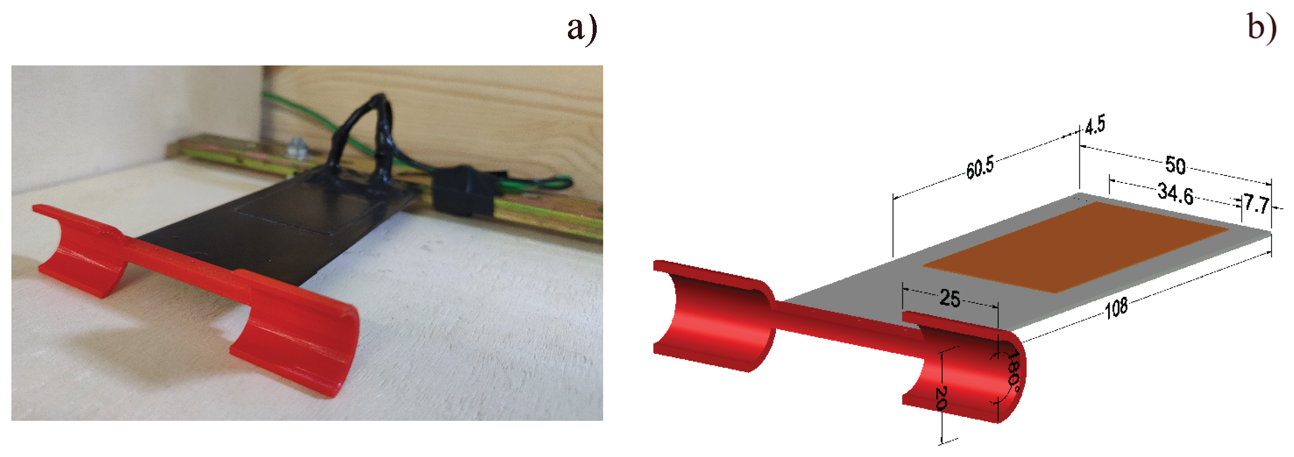
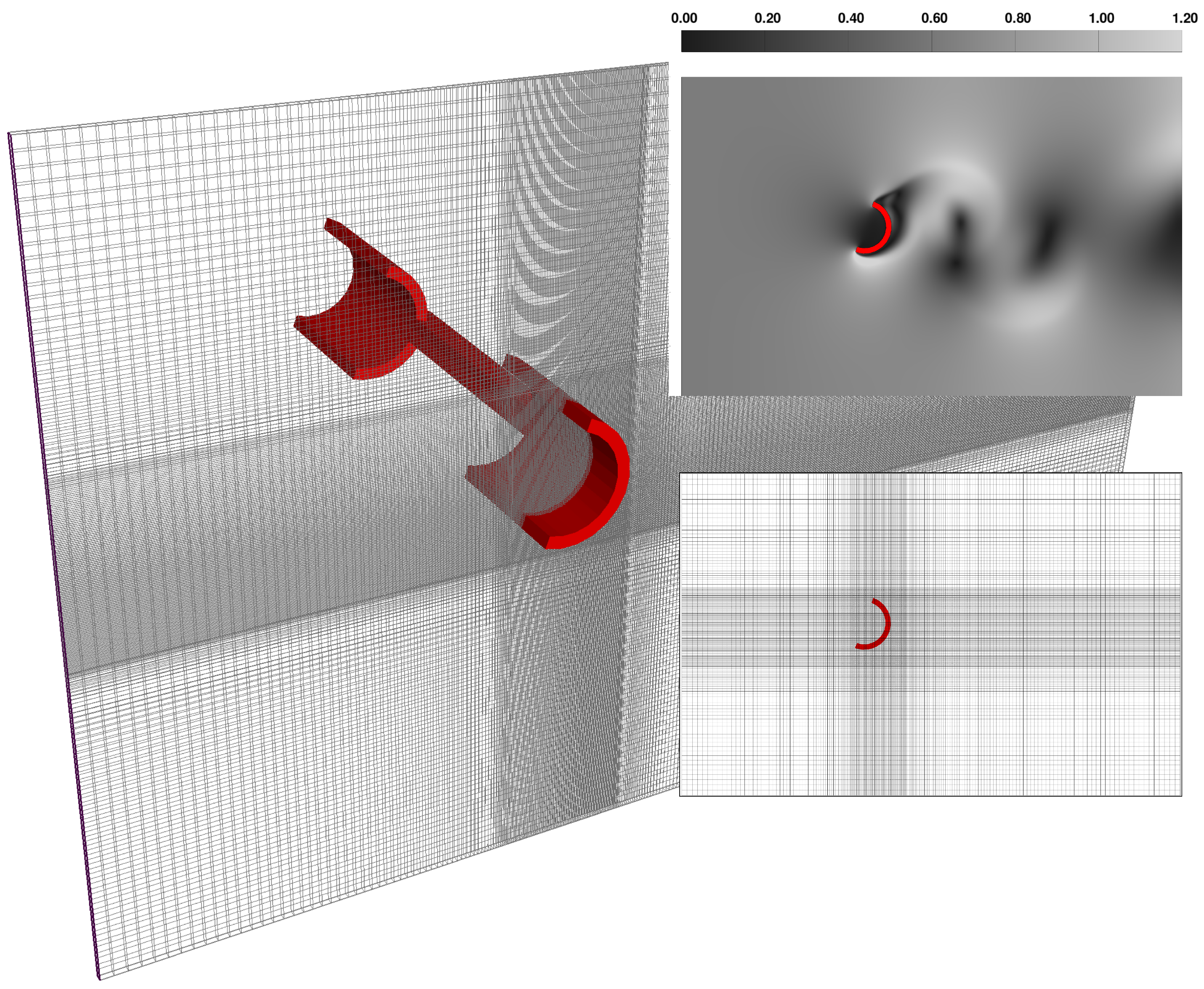
2.1. CFD Modelling of the FSI for the VI

In the following, we describe the procedure to determine the force exerted by the fluid on the VI alone.

Such force is calculated numerically by means of a CFD (Computational Fluid Dynamics) analysis as the one acting on the VI at rest at various AoA $\alpha$ and different undisturbed flow velocities $U_{\infty }$.

The CFD model is a commercially available package [32] solving for RANS on structured, non uniform grids. The C-shaped section of the VI wings has been placed in a steady, uniform water flow with its concave side facing upstream. The numerical experiments covered a range of flow velocity $U_{\infty }$ and AoA $\alpha$ of $0.567\mathrm{m}/\mathrm{s}<U_{\infty }<0.693\mathrm{m}/\mathrm{s}$ and $0\mathrm{deg}<\alpha <20\mathrm{deg}$ with increments of $\Delta U_{\infty }=0.0315\mathrm{m}/\mathrm{s}$, $\Delta \alpha =5\mathrm{deg}$, resulting in a total of 25 simulations. Although the model has been extensively benchmarked, a further validation was carried out: the reference drag coefficients of the two-dimensional semitubular cylinder of diameter $D=16$ mm at null AoA, as reported in [33,34], was calculated with a maximum error of 2%.

With reference to Figure 2, the domain extends $4\times D$ upstream, $7\times D$ downstream, and $3.5\times D$ cross flow. The same grid, determined through a grid convergence analysis, was employed for all simulations. The cartesian, non-uniform grid features a spacing ranging from $D/8$ at the boundaries, to $D/64$ around the object, resulting in $4.3\times {10}^4$ elements. Boundary conditions were of uniform, constant velocity upstream, uniform and constant pressure downstream and symmetrical conditions crossflow. The turbulence closure model yielding best results in the validation phase was the $k-\omega$ one [35], and it is then adopted in the simulations. In the analysed flow regimes, characterized by a Reynolds number $Re=U_{\infty }D/\nu \simeq {10}^4$, $\nu$ being the kinematic viscosity, a regularly oscillating vortex shedding develops in the wake. The simulations were run until the wake attained a permanent oscillation. Drag and lift time histories acting on the VI were extracted and their time-averaged values, referred to respectively as $F_D,F_L$ in the following, passed to the beam structural model.

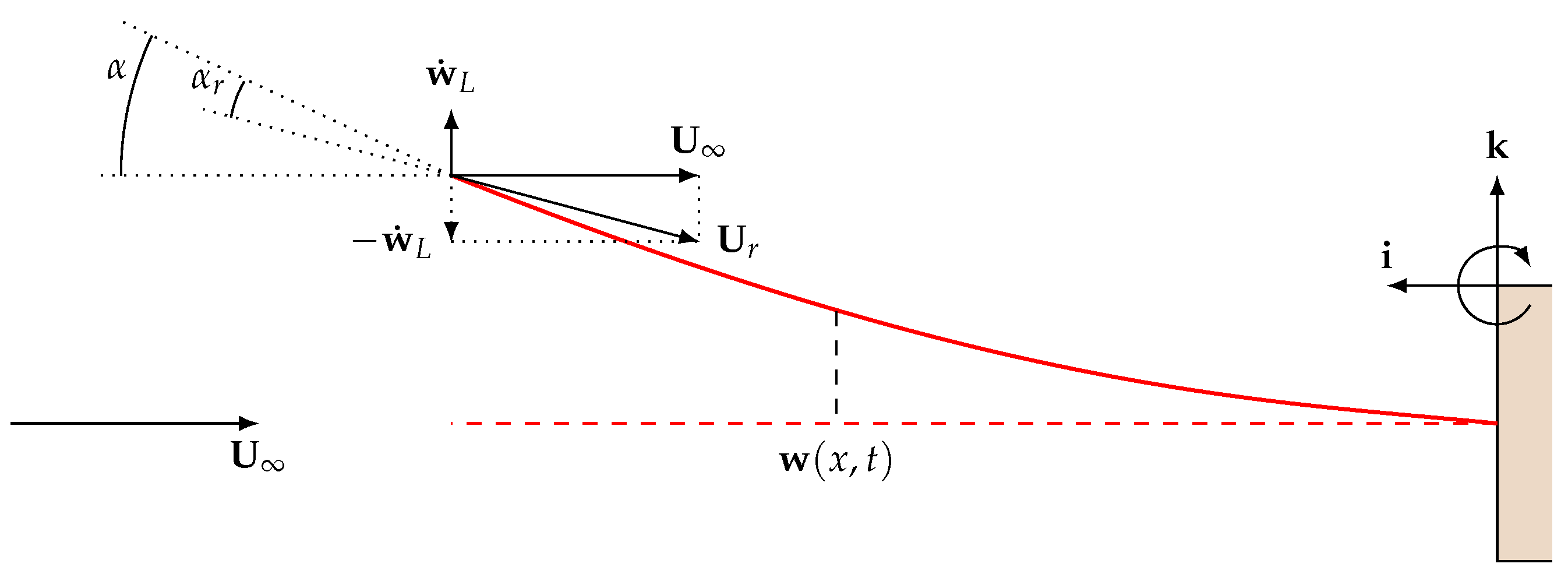
2.2. The Beam Model: Modified Euler-Bernoulli Equation

The classical Euler-Bernoulli (EB) beam equation is here modified to account for the longitudinal forces (i.e., parallel to $U_{\infty }$ and to the beam rest position as in Figure 3) exerted by the VI mounted on the tip of the beam. Let x be such direction and $w\left(x,t\right)$ the beam displacement at position x and time t.

In the following, prime and dot notations stand for space and time differentiation, respectively. Moreover, bold symbols are used for vector quantities. The standard EB equation can be written as:

$$\rho S\ddot{w}\left(x,t\right)+EJ{w}^{⁗}\left(x,t\right)=\mathcal{F}\left(x,t\right),$$

(1)

where $\rho$ and E are, respectively, density and elastic modulus of the beam material, while S and J are the area and the second moment of area with respect to the neutral axis of the beam cross-section; $\mathcal{F}\left(x,t\right)$ is the transverse load distributed along the beam length L. Numerical values for $\rho$, S and E are the ones of an homogeneous beam equivalent to the monomorph piezoelectric beam according to the homogenization procedure described in Appendix A. The fourth order term in the Equation (1) can be written as $EJ{w}^{⁗}\left(x,t\right)=M^{″}\left(x,t\right)$ where $M\left(x,t\right)$ is the bending moment due to the applied transverse load. A longitudinal force $F_l$, i.e., aligned with the direction of the undisturbed flow velocity, applied to beam’s free end ($x=L$) yields a further bending moment $M_l\left(x,t\right)$:

$$M_l\left(x,t\right)=-F_l\left[w\left(L,t\right)-w\left(x,t\right)\right].$$

(2)

As a consequence:

$$M_l^{″}\left(x,t\right)=F_l{w}^{″}\left(x,t\right).$$

(3)

To tackle the problem through a modal analysis, transverse forces $F_t$ exerted by the VI and its inertia need to be accounted for as loads on the bulk, by means of standard Dirac-Delta functions. The resulting modified EB beam equation reads:

$$\left[\rho S+m\delta \left(x-L\right)\right]\ddot{w}\left(x,t\right)+EJ{w}^{⁗}\left(x,t\right)+F_l{w}^{″}\left(x,t\right)=F_t\delta \left(x-L\right)+\mathcal{F}\left(x,t\right),$$

(4)

where m is the mass of the VI.

Standard boundary conditions for a cantilever, together with the following initial conditions are applied:

$$\left\{\begin{array}{c}w(0,t)=w^{\prime }(0,t)=0,\hfill \\ w^{″}(L,t)=w^{‴}(L,t)=0,\hfill \\ w(x,0)=w_0\left(x\right),\dot{w}(x,0)=v_0\left(x\right).\hfill \end{array}\right.$$

(5)

where $w_0\left(x\right)$ and $v_0\left(x\right)$ describe assigned initial position and motion distributions which can be employed as a perturbation to trigger the subsequent oscillation.

In Section 2.3, $F_l$, $F_t$ will be derived from the static ones determined by means of the CFD modelling in Section 2.1. As stated in the introduction, due to the particular shape of the employed VI, the distributed load $\mathcal{F}\left(x,t\right)$, i.e., the direct action of the fluid on the beam, will be proven to be pivotal for replicating the experimental results.

2.3. The Quasi Steady Forcing

The drag and lift components provided by the CFD model, as described in Section 2.1, are determined considering the VI at rest, therefore the total force ${\mathbf{F}}_{stat}$ depends on the undisturbed upstream flow velocity $U_{\infty }$ and on the VI AoA $\alpha$, namely:

$${\mathbf{F}}_{stat}\left(U_{\infty },\alpha \right)=-F_D\left(U_{\infty },\alpha \right)\mathbf{i}+F_L\left(U_{\infty },\alpha \right)\mathbf{k},$$

(6)

where $\mathbf{i}$ and $\mathbf{k}$ are the unit vectors, respectively, of the x and z axes as depicted in Figure 3. The evaluation of the force acting on the moving VI needs to account for its instantaneous AoA and velocity. Being the VI mounted on the tip of the oscillating beam, its instantaneous configuration can be described in terms of the motion and orientation of the tip. With reference to Figure 3, the quasi steady assumption is here enforced, which states that the force ${\mathbf{F}}_{dyn}$ acting on the VI during its motion can be determined from the components of the static force in Equation (6) as:

$${\mathbf{F}}_{dyn}\left(U_r,{\alpha }_r\right)=-F_D\left(U_r,{\alpha }_r\right){\mathbf{i}}_r+F_L\left(U_r,{\alpha }_r\right){\mathbf{k}}_r,$$

(7)

where the relative velocity ${\mathbf{U}}_r$, the relative AoA ${\alpha }_r$ depend on the tip motion and orientation as follows:

$$\left\{\begin{array}{c}{\mathbf{U}}_r=-U_{\infty }\mathbf{i}-\dot{w}(L,t)\mathbf{k},\hfill \\ {\alpha }_r=\underset{\alpha }{\underbrace{arctan\left[w^{\prime }(L,t)\right]}}-arcsin\left(\frac{\dot{w}(L,t)}{U_r}\right).\hfill \end{array}\right.$$

(8)

and the unit vectors ${\mathbf{i}}_r,{\mathbf{k}}_r$ are respectively aligned and perpendicular to ${\mathbf{U}}_r$, and depend on the tip motion as:

$$\left\{\begin{array}{c}{\mathbf{i}}_r\equiv \frac{U_{\infty }\mathbf{i}+\dot{w}(L,t)\mathbf{k}}{U_r}\hfill \\ {\mathbf{k}}_r\equiv -sgn\left({\alpha }_r\right)\frac{-\dot{w}(L,t)\mathbf{i}+U_{\infty }\mathbf{k}}{U_r}\hfill \end{array}\right.$$

(9)

$F_l$ and $F_t$ appearing in Equation (4) are the longitudinal and transverse components of ${\mathbf{F}}_{dyn}$, that is:

$$\left\{\begin{array}{c}{F}_l={\mathbf{F}}_{dyn}·\mathbf{i},\hfill \\ F_t={\mathbf{F}}_{dyn}·\mathbf{k}.\hfill \end{array}\right.$$

(10)

To compute them, according to Equations (7) and (8), the domain $(U_{\infty },\alpha )$ needs to be continuously sampled. Therefore, the discrete values of $F_D$ and $F_L$ as yielded by the CFD simulations have been suitably interpolated. For a comprehensive discussion on the effect of such interpolation, the reader is referred to [36] and to the works therein cited.

Quasi steady modelling of the galloping motion of such devices has been extensively employed $10/1$ [15,18,20,36,37,38,39], being supported by the difference in peak frequencies between vortex shedding in the wake of the VI ($f_{\mathrm{VI}}$) and oscillation of the FEH ($f_{\mathrm{FEH}}$). In our case, the two stand in the ratio $f_{\mathrm{VI}}/f_{\mathrm{FEH}}\simeq 4:1$.

The moment $M_{dyn}$, as computed from the above described quasi steady assumption, resulted to be negligible for the case considered (i.e., $\left|L{F}_{dyn}/M_{dyn}\right|\gg 1$), and it has not been included in the modelling.

2.4. The Experimental Setup

The performance of the a wide class of C-shaped VIs has been experimentally tested in a free surface flume by means of experimental FEHs [27,28,40] like the one shown in Figure 1, where both a picture and a sketch of the FEH employed in this work, along with its dimensions in mm, are provided.

The cantilever is placed counterflow at the centerline of the channel parallel to its lateral walls. It is made of a steel foil clamped at one end to form a $10.8$ cm long cantilever. A ceramic perovskite (PZT) piezoelectric plate of weigth 2.05 g made by Physik Instrumente [41] is glued on the top face of the lamina. A differential probe connected to an oscilloscope is employed for the acquisition of the AC electrical voltage produced by the piezoelectric patch deformation under flow induced oscillations. The experiments are carried out with an open circuit configuration. For further details on the employed experimental configuration the reader is referred to [27,28]. Figure 4 shows the transverse displacement of the tip of the cantilever detected by image analysis for a duration of 45 s. The inset shows the comparison between the measured signal and the sine function employed to fit the experimental data. Specifically, an amplitude $a=0.0089$ m and a frequency $f=3.6$ Hz have been used to obtain the fitting function. It is worth highlighting that, in force of Equation (8), the maximum rotation of the tip section of the beam during the employed experimental runs (namley 6 deg) is considerably smaller than the maximum AoA (namely 20 deg) investigated within the CFD runs in Section 2.1. The above supports the employment of the linear Euler-Bernoulli model.

2.5. Finite Dimensional Approach and Galerkin Expansion

We expand the solution of the partial differential equation Equation (4) into its eigenfunctions series:

$$w\left(x,t\right)=\sum _{i=1}^{\infty }{A}_i\left(t\right)z_i\left(x\right),$$

(11)

where ${\left\{z_i\left(x\right)\right\}}_{i=1,2,\dots }$ are the eigenfunctions of the standard EB equation for the cantilever [42]. Inserting the expansion, Equation (11), into the differential equation Equation (4) and retaining only the first mode $A_1\left(t\right)z_1\left(x\right)$, after a Galerkin projection, the following nonlinear second order ordinary differential equation in the unknown $A_1\left(t\right)$ is obtained:

$${\ddot{A}}_1\left(t\right)+\frac{{\mathcal{N}}_{12}}{\zeta }{F}_l{A}_1\left(t\right)+\frac{{\omega }_{10}^2}{\left(1+\chi \right)}{A}_1\left(t\right)=\frac{z_1\left(L\right)}{\zeta }{F}_t+\frac{\left(\mathcal{F},z_1\left(x\right)\right)}{\zeta },$$

(12)

where:

$$\left\{\begin{array}{c}(▵,\square )\equiv {\int }_0^L\Delta \square dx,\hfill \\ {\mathcal{N}}_{12}\equiv \left(z_1,z_1^{″}\right),\hfill \\ {\mathcal{N}}_{11}\equiv \left(z_1,z_1\right),\hfill \\ \chi \equiv \frac{m{z}_1^2\left(L\right)}{\rho S{\mathcal{N}}_{11}}\hfill \\ \zeta \equiv \rho S(1+\chi ){\mathcal{N}}_{11}.\hfill \end{array}\right.$$

(13)

and ${\omega }_{10}$ is the natural angular frequency of the first eigenmode of the piezoelectric-beam system. In Equation (12) $F_t$ and $F_l$, owing to Equations (10), (7) and (11), are non linear functions of $A_1\left(t\right),\dot{A_1}\left(t\right)$. Finally, the term $\left(\mathcal{F},z_1\left(x\right)\right)/\zeta$ models the distributed transverse load along the beam due to the direct fluid dynamic action. The distributed load of the fluid onto the beam is expected to be extremely complex, resulting from the presence of multiple eddies generated by the non-stationary wake of the tip of beam. Such dynamics rules out the employment of simple, yet physically based, formulations. Therefore, the term will be modeled assuming that it can be expressed at leading order as a linear combination of $A_1\left(t\right)$ and $\dot{A_1}\left(t\right)$ according to:

$$\left(\mathcal{F},z_1\left(x\right)\right)/\zeta =2\gamma {\omega }_{10}\dot{A_1}\left(t\right)+\beta \left(\frac{{\rho }_f{U}_{\infty }^2}{\rho S}\right)A_1\left(t\right),$$

(14)

where $\gamma$ and $\beta$ are dimensionless calibration parameters of the model, and ${\rho }_f$ is the fluid density.

3. Results

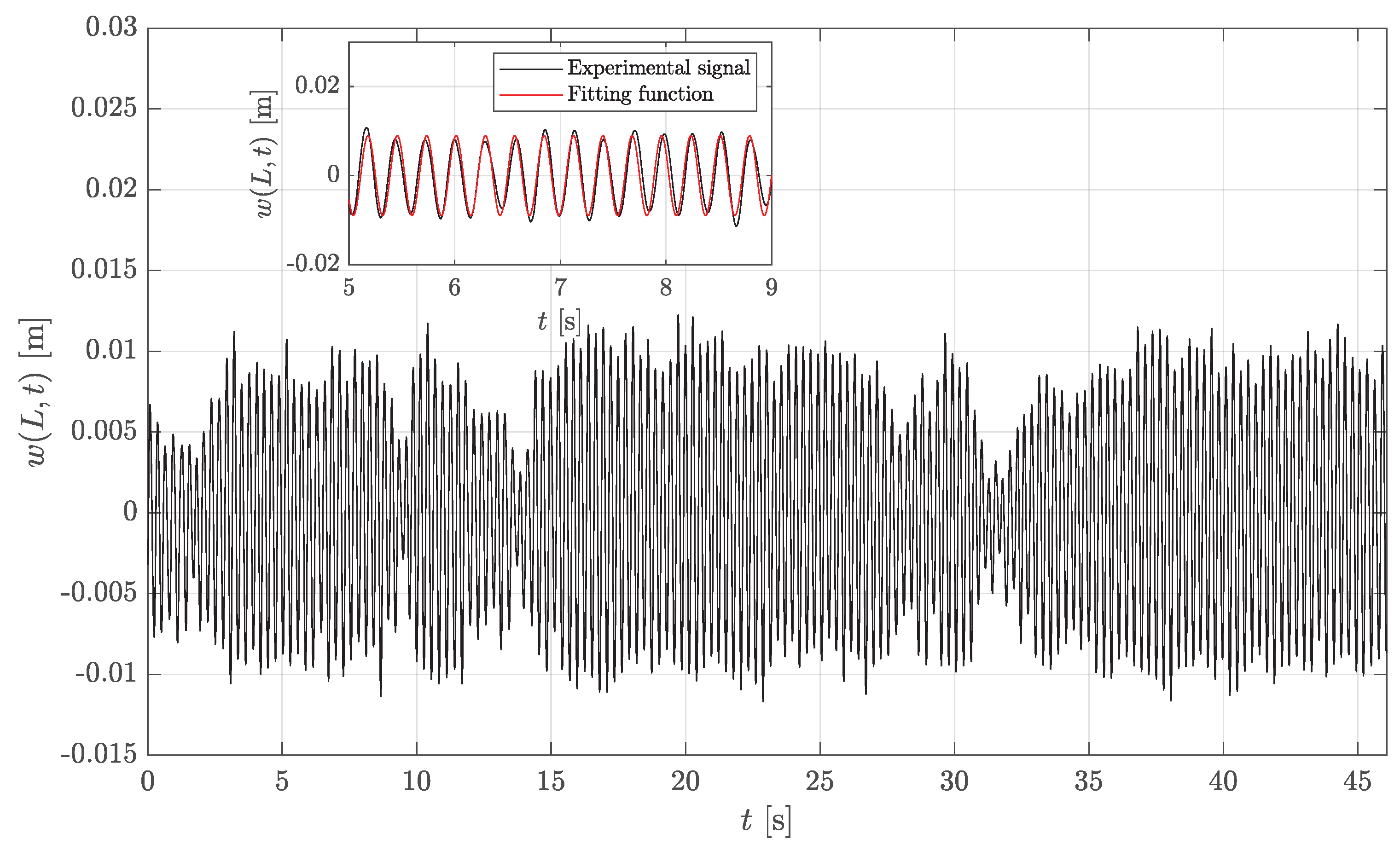
3.1. Model Calibration against Experimental Results

The model described by Equation (12) has two free parameters as defined in Equation (14), namely $\gamma$ and $\beta$. Both terms describe the fluid action exerted directly on the beam, the first one being proportional to the velocity of the beam, the second to its position. The rationale behind such modelling choice lies in allowing for both a bidirectional ($\beta$-term) and a unidirectional ($\gamma$-term) net power transfer between beam and fluid, in a single cycle, in the limit of harmonic swaying.

The values of the two free parameters have been determined through a minimization procedure of a loss function between the experimental and the numerical spectra. The best set of parameters yields the results in Figure 5, where the leading frequency of the oscillation can be reproduced with an error of $0.1$%. The comparison of time histories of tip motion, showing a marked match of the amplitude as well, confirms the correctness of the calibration procedure. The best fit values of $\gamma$ and $\beta$ are 0.0626 and 3.11, respectively. As will be demonstrated in the next section, this implies that in whole oscillation, a net power transfer takes place directly from the fluid to the beam.

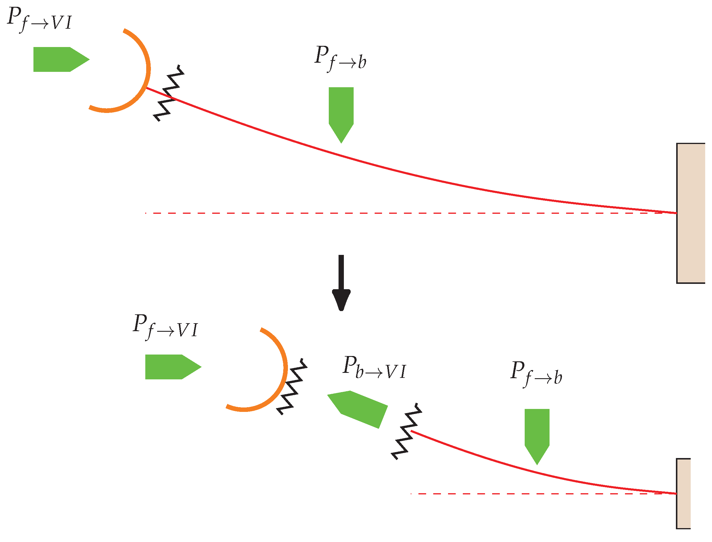
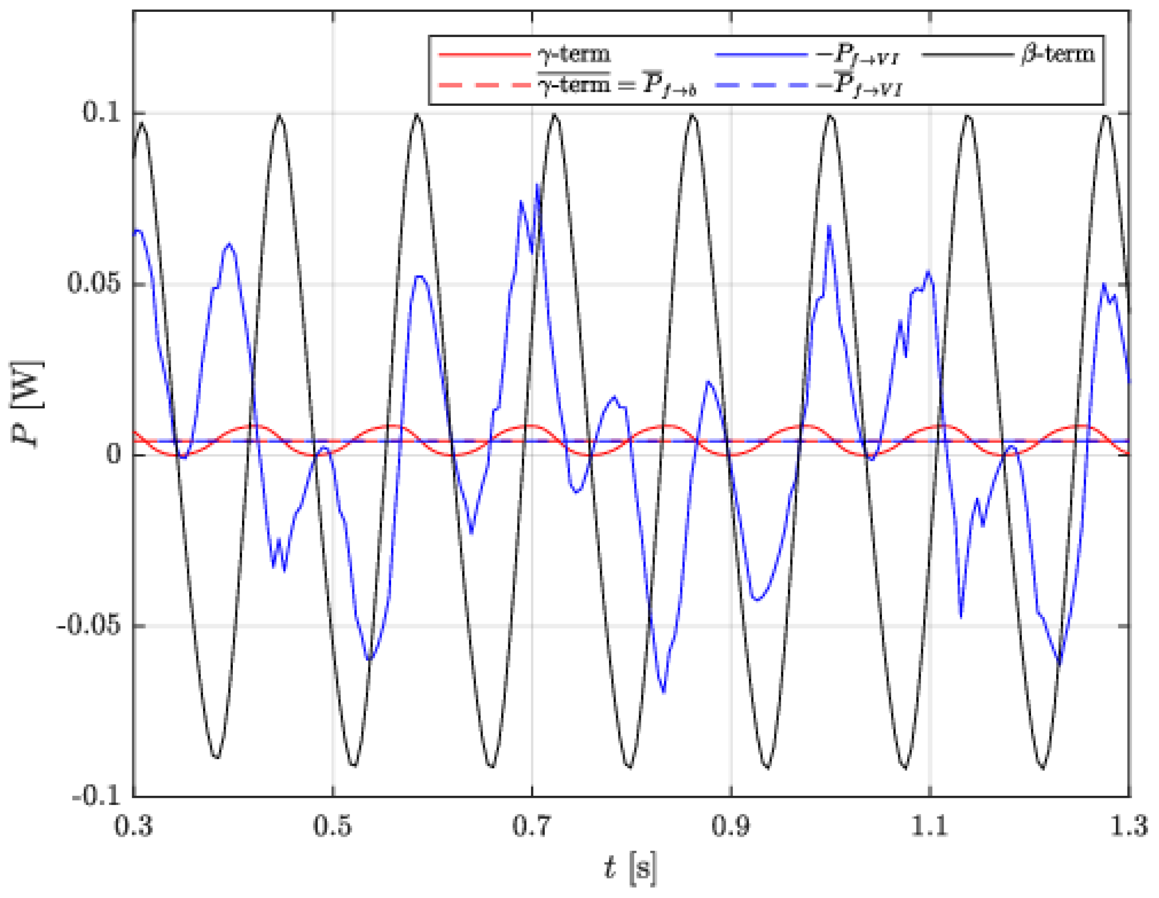
3.2. Evaluation of the Work Done by Fluid Forces on the VI

A validation of the attained calibration is carried out by comparing the power transfers between the fluids and the different parts of the FEH, namely the VI and the beam. With reference to Figure 6, assuming the VI to oscillate only along y direction, the instantaneous power transfer $P_{f\to VI}$ from fluid to the VI reads:

$$P_{f\to VI}=F_t\dot{w}\left(L,t\right).$$

(15)

Let $P_{b\to VI}$ be the power transferred by the beam tip to VI. Then the change in kinetic energy $d{K}_{VI}$ in a time interval $dt$ of the VI reads:

$$d{K}_{VI}=\left(P_{b\to VI}+P_{f\to VI}\right)dt.$$

(16)

Assuming the motion to be purely harmonic (as approximately highlighted by experimental measurements and shown by numerical solution of Equation (12)), the variation of kinetic energy $\Delta K_{VI}$ over an integer number of periods ($nT,n=1,2,\dots$) must vanish, that is:

$$\Delta K_{VI}=0={\int }_0^{nT}{P}_{b\to VI}dt+{\int }_0^{nT}{P}_{f\to VI}dt.$$

(17)

By dividing Equation (17) by $nT$, the two terms on the RHS represent the power transferred to the VI by the beam and by the fluid, averaged over an integer number of periods. These two mean values of power, referred to as ${\overline{P}}_{b\to VI}$ and ${\overline{P}}_{f\to VI}$ respectively, must satisfy the following balance:

$${\overline{P}}_{b\to VI}=-{\overline{P}}_{f\to VI}.$$

(18)

In the following, Equation (18) will be verified to hold with remarkable accuracy. Such match will support our thesis that the direct action of the fluid on the beam, as formulated in Equation (14), must be included in the model, Equations (12), to achieve an accurate agreement with experimental results as depicted in Figure 5.

Firstly, ${\overline{P}}_{f\to VI}$ has been estimated through a CFD simulation encompassing a harmonically moving VI. The simulation has been carried out by means of the same software employed in Section 2.1. The time history of $P_{f\to VI}$ is shown in Figure 7.

As per the term ${\overline{P}}_{b\to VI}$, in the limit of negligible damping occurring in the beam (it is here worth recalling that the experiments are carried out employing an open circuit electrical configuration), it is equal to the power that the fluid transfers to the beam, namely ${\overline{P}}_{f\to b}$. As such, it can be readily calculated by solving Equation (12) for $A_1\left(t\right)$, multiplying it by ${\dot{A}}_1\left(t\right)$ and then integrating over an integer number of periods. Owing to Equation (14), such average power can be calculated as follows:

$${\overline{P}}_{b\to VI}\equiv {\overline{P}}_{f\to b}=\frac{\zeta }{nT}{\int }_0^{nT}2\gamma {\omega }_{10}{\dot{A}}_1{\left(t\right)}^2+\beta \left(\frac{{\rho }_f{U}_{\infty }^2}{\rho S}\right)A_1\left(t\right){\dot{A}}_1\left(t\right)dt=2\gamma \zeta {\omega }_{10}\overline{{\dot{A}}_1{\left(t\right)}^2},$$

(19)

where the $\beta$-term in Equation (14) does not contribute to the average since the product of the harmonic functions $A_1\left(t\right){\dot{A}}_1\left(t\right)$ vanishes after integration. The time histories of these two contributions to the power $P_{f\to b}$ are included in Figure 7.

Finally, Equation (18) reads:

$$2\gamma \zeta {\omega }_{10}\overline{\dot{A_1}{\left(t\right)}^2}=-{\overline{P}}_{f\to VI}.$$

(20)

The above calculation allows to verify that Equation (18) holds within a $4\%$ error. Figure 7 shows the time histories of the power fluxes employed in the above verification. It is worth highlighting that the commonly employed approach to the modelling of FEH, which accounts for the VI as the only driver of the beam oscillation, is found by the authors to yield largely inconsistent results when compared to the experimental data. Indeed, the investigated shape of the VI requires the inclusion of the two additional terms in Equation (14), whose omission prevents the correct closure of the power balance within a cycle motion.

Moreover, the following considerations are in order. The model is forced by the time averaged values of the time-dependent forces acting on the VI, namely the $F_l$ and $F_t$ in Equation (12). Therefore, the model cannot be expected to replicate the time modulation of the $P_{f\to VI}$ term as shown in Figure 7, which is the result of the CFD modelling and includes all the time-dependent effects induced by the vortex shedding. Nonetheless, the time-averaged values of the power transfer is reproduced with remarkable accuracy. Such a match validates the present model as a valuable tool for designing and testing FEHs. Indeed, such analyses are mainly focused on evaluating the harvestable power over many oscillating cycles, which the present model is able to capture satisfactorily.

4. Conclusions

In this work, we model the Fluid Structure Interaction (FSI) problem arising from the behavior of a particular Flow Energy Harvester (FEH) featuring an innovative Vibration Inducer (VI). The latter is shaped as a semitubular cylinder with the concave side facing upstream and makes the attached cantilever oscillate regularly in a steady flow. Such shape of the VI is aimed at: (i) exploiting the longitudinal drag force ii) allowing for the undisturbed upstream flow to impinge directly on the cantilever. Given such peculiar dynamics, a novel modelling strategy had to be devised, accounting for i) the additional bending moment induced by the longitudinal forces acting on the VI; (ii) the direct (i.e., not mediated by the VI) action of the fluid on the beam. The latter is modelled as the sum of a positional and a velocity term, whose governing parameters are calibrated against experimental results. The action of the fluid on the VI is estimated by means of a numerical CFD analysis, enforcing the usual quasi-steady assumption. The model is validated by comparing its outcomes with the ones yielded by further CFD analyses encompassing the simulated motion of the VI. The match, in terms of average power over a multiple of the swaying cycle, is remarkable, notwithstanding the adopted minimal modelling of the complex interaction occurring between the fluid and the beam. The proposed model is a valuable tool to analyse the dynamic response of such class of Flow Energy Harvester and significantly aid their design procedure. Future studies will be devoted to a possible refinement of the form of the terms accounting for direct fluid–beam interaction.

References

1. Lu, F.; Lee, H.P.; Lim, S.P. Modeling and analysis of micro piezoelectric power generators for micro-electromechanical-systems applications. Smart Mater. Struct. 2003, 13, 57. [Google Scholar] [CrossRef]
2. Cook-Chennault, K.A.; Thambi, N.; Sastry, A.M. Powering MEMS portable devices—A review of non-regenerative and regenerative power supply systems with special emphasis on piezoelectric energy harvesting systems. Smart Mater. Struct. 2008, 17, 043001. [Google Scholar] [CrossRef] [Green Version]
3. St Clair, D.; Bibo, A.; Sennakesavababu, V.R.; Daqaq, M.F.; Li, G. A scalable concept for micropower generation using flow-induced self-excited oscillations. Appl. Phys. Lett. 2010, 96, 144103. [Google Scholar] [CrossRef]
4. Huang, G.; Xia, Y.; Dai, Y.; Yang, C.; Wu, Y. Fluid–structure interaction in piezoelectric energy harvesting of a membrane wing. Phys. Fluids 2021, 33, 063610. [Google Scholar] [CrossRef]
5. Alam, M.M.; Chao, L.-M.; Rehamn, S.; Ji, C.; Wang, H. Energy harvesting from passive oscillation of inverted foil. Phys. Fluids 2021, 33, 075111. [Google Scholar] [CrossRef]
6. Pobering, S.; Schwesinger, N. A novel hydropower harvesting device. In Proceedings of the International Conference on MEMS, NANO and Smart Systems (ICMENS 04), Banff, AB, Canada, 25–27 August 2004; pp. 480–485. [Google Scholar]
7. Kouritem, S.A.; Bani-Hani, M.A.; Beshir, M.; Elshabasy, M.M.Y.B.; Altabey, W.A. Automatic Resonance Tuning Technique for an Ultra-Broadband Piezoelectric Energy Harvester. Energies 2022, 15, 7271. [Google Scholar] [CrossRef]
8. Renno, J.M.; Daqaq, M.F.; Inman, D.J. On the optimal energy harvesting from a vibration source. J. Sound Vib. 2009, 320, 386–405. [Google Scholar] [CrossRef]
9. Ma, X.; Zhou, S. A review of flow-induced vibration energy harvesters. Energy Convers. Manag. 2022, 254, 115223. [Google Scholar] [CrossRef]
10. Akaydin, H.D.; Elvin, N.; Andreopoulos, Y. Energy harvesting from highly unsteady fluid flows using piezoelectric materials. J. Intell. Mater. Syst. Struct. 2010, 21, 1263–1278. [Google Scholar] [CrossRef]
11. Tang, D.M.; Yamamoto, H.; Dowell, E.H. Flutter and limit cycle oscillations of two-dimensional panels in three-dimensional axial flow. J. Fluids Struct. 2003, 17, 225–242. [Google Scholar] [CrossRef]
12. Hassan, M.M.; Hossain, M.Y.; Mazumder, R.; Rahman, R.; Rahman, M.A. Vibration energy harvesting in a small channel fluid flow using piezoelectric transducer. AIP Conf. Proc. 2016, 1754, 050041. [Google Scholar]
13. Akaydin, H.D.; Elvin, N.; Andreopoulos, Y. The performance of a self-excited fluidic energy harvester. J. Intell. Mater. Syst. Struct. 2012, 21, 025007. [Google Scholar] [CrossRef]
14. Seyed-Aghazadeh, B.; Samandari, H.; Dulac, S. Flow-induced vibration of inherently nonlinear structures with applications in energy harvesting. Phys. Fluids 2020, 32, 071701. [Google Scholar] [CrossRef]
15. Hamlehdar, M.; Kasaeian, A.; Safaei, M.R. Energy harvesting from fluid flow using piezoelectrics: A critical review. Renew. Energy 2019, 143, 1826–1838. [Google Scholar] [CrossRef]
16. Naqvi, A.; Ali, A.; Altabey, W.A.; Kouritem, S.A. Energy Harvesting from Fluid Flow Using Piezoelectric Materials: A Review. Energies 2022, 15, 7424. [Google Scholar] [CrossRef]
17. Forouzi Feshalami, B.; He, S.; Scarano, F.; Gan, L.; Morton, C. A review of experiments on stationary bluff body wakes. Phys. Fluids 2022, 34, 011301. [Google Scholar] [CrossRef]
18. Jo, S.; Sun, W.; Son, C.; Seok, J. Galloping-based energy harvester considering enclosure effect. AIP Adv. 2018, 8, 095309. [Google Scholar] [CrossRef]
19. Bibo, A.; Abdelkefi, A.; Daqaq, M.F. Modeling and characterization of a piezoelectric energy harvester under combined aerodynamic and base excitations. J. Vib. Acoust. 2015, 137, 031017. [Google Scholar] [CrossRef]
20. Yang, Y.; Zhao, L.; Tang, L. Comparative study of tip cross-sections for efficient galloping energy harvesting. Appl. Phys. Lett. 2013, 102, 064105. [Google Scholar] [CrossRef]
21. Elvin, N.; Erturk, A. Advances in Energy Harvesting Methods; Springer: New York, NY, USA, 2013. [Google Scholar]
22. Wang, J.; Zhou, S.; Zhang, Z.; Yurchenko, D. High-performance piezoelectric wind energy harvester with Y-shaped attachments. Energy Convers. Manag. 2019, 181, 645–652. [Google Scholar] [CrossRef]
23. Parkinson, G.V.; Brooks, N.P.H. On the aeroelastic instability of bluff cylinders. J. Appl. Mech. 1961, 28, 252–258. [Google Scholar] [CrossRef]
24. Parkinson, G.V.; Smith, J.D. The square prism as an aeroelastic non-linear oscillator. Q. J. Mech. Appl. Math. 1964, 17, 225–239. [Google Scholar] [CrossRef]
25. Song, J.; Hu, G.; Tse, K.T.; Li, S.W.; Kwok, K.C.S. Performance of a circular cylinder piezoelectric wind energy harvester fitted with a splitter plate. Appl. Phys. Lett. 2017, 111, 223903. [Google Scholar] [CrossRef]
26. Curatolo, M.; La Rosa, M.; Prestininzi, P. Energy harvesting in a fluid flow using piezoelectric material. In Proceedings of the 2018 COMSOL Conference, Lausanne, Switzerland, 22–24 October 2018. [Google Scholar]
27. Curatolo, M.; Lombardi, V.; Prestininzi, P. Enhancing flow induced vibrations of a thin piezoelectric cantilever: Experimental analysis. In Proceedings of the International Conference on Fluvial Hydraulics River Flow 2020, Delft, The Netherlands, 6–17 July 2020. [Google Scholar]
28. Lombardi, V.; La Rocca, M.; Prestininzi, P. A new dynamic masking technique for time resolved PIV analysis. J. Vis. 2021, 24, 979–990. [Google Scholar] [CrossRef]
29. Tucker Harvey, S.; Khovanov, I.A.; Denissenko, P. A galloping energy harvester with flow attachment. Appl. Phys. Lett. 2019, 114, 104103. [Google Scholar] [CrossRef] [Green Version]
30. Tucker Harvey, S.; Khovanov, I.A.; Murai, Y.; Denissenko, P. Characterisation of aeroelastic harvester efficiency by measuring transient growth of oscillations. Appl. Energy 2020, 268, 115014. [Google Scholar] [CrossRef]
31. Shi, T.; Gang, H.; Lianghao, Z. Aerodynamic Shape Optimization of an Arc-Plate-Shaped Bluff Body via Surrogate Modeling for Wind Energy Harvesting. Appl. Sci. 2022, 12, 3965. [Google Scholar] [CrossRef]
32. FLOW-3D, Version 12.0; Flow Science, Inc.: Santa Fe, NM, USA, 2019; Available online: https://www.flow3d.com/ (accessed on 1 January 2020).
33. Lindsey, W.F. Drag of cylinders of simple shapes. NACA Tech. Rep. 1938, 619, 169–176. [Google Scholar]
34. Hoerner, S.F. Fluid Dynamic Drag; Hoerner Fluid Dynamics: Bakersfield, CA, USA, 1965. [Google Scholar]
35. Wilcox, D.C. Turbulence Modeling for CFD; 3DCW Industries: La Canada, CA, USA, 1998. [Google Scholar]
36. Javed, U.; Abdelkefi, A. Impacts of the aerodynamic force representation on the stability and performance of a galloping-based energy harvester. J. Sound Vib. 2017, 400, 213–226. [Google Scholar] [CrossRef]
37. Blevins, R. Flow-Induced Vibration; Van Nostrand Reinhold: New York, NY, USA, 1990. [Google Scholar]
38. Barrero-Gil, A.; Alonso, G.; Sanz-Andres, A. Energy harvesting from transverse galloping. J. Sound Vib. 2010, 329, 2873–2883. [Google Scholar] [CrossRef] [Green Version]
39. Bibo, A.; Daqaq, M.F. An analytical framework for the design and comparative analysis of galloping energy harvesters under quasi-steady aerodynamics. Smart Mater. Struct. 2015, 24, 094006. [Google Scholar] [CrossRef]
40. Curatolo, M.; La Rosa, M.; Prestininzi, P. On the validity of plane state assumptions in the bending of bimorph piezoelectric cantilevers. J. Intell. Mater. Syst. Struct. 2019, 30, 1508–1517. [Google Scholar] [CrossRef]
41. Physik Instrumente. Available online: https://www.physikinstrumente.com/en/ (accessed on 14 November 2022).
42. Blevins, R. Wave Motion in Elastic Solids; VDover Publications Inc.: New York, NY, USA, 2003. [Google Scholar]
Figure 1. Picture of the experimental FEH (a); the red VI in the foreground is mounted on the tip of the beam, the latter being coated with black paint. Sketch of the FEH (b); all dimensions are in mm.
Applsci 13 00416 g001
Figure 2. 3D and 2D view (lower inset) of the non-uniform grid employed in the CFD code. Upper inset: example of flow field (velocity magnitude in m/s). The VI is depicted in red.
Applsci 13 00416 g002
Figure 3. Sketch of the quantities appearing in the model formulation.
Applsci 13 00416 g003
Figure 4. Experimental signal: transverse displacement of beam tip. The inset shows the overlapping of the harmonic fitting function with the experimental recording for the time interval 5 s < t < 9 s.
Applsci 13 00416 g004
Figure 5. Comparison between experimental (black line) and numerical results (red line): time history of the tip motion (a) and frequency spectrum of the tip motion (b).
Applsci 13 00416 g005
Figure 6. Power flows between the fluid and the FEH. To assess the accuracy of the modelling of the power transfer from the fluid to the beam, it is compared to the one transferred from the VI to the beam, the latter emerging as an internal power flow once the FEH is thought as composed by the VI and the beam.
Applsci 13 00416 g006
Figure 7. Comparison among power terms. γ and β -terms refer to the instantaneous power linked to the RHS of Equation (14); mean value γ - term ¯ is the power transfer in Equation (19).
Applsci 13 00416 g007
Disclaimer/Publisher’s Note: The statements, opinions and data contained in all publications are solely those of the individual author(s) and contributor(s) and not of MDPI and/or the editor(s). MDPI and/or the editor(s) disclaim responsibility for any injury to people or property resulting from any ideas, methods, instructions or products referred to in the content.