A Nighttime and Daytime Single-Image Dehazing Method

Abstract

In this study, the requirements for image dehazing methods have been put forward, such as a wider range of scenarios in which the methods can be used, faster processing speeds and higher image quality. Recent dehazing methods can only unilaterally process daytime or nighttime hazy images. However, we propose an effective single-image technique, dubbed MF Dehazer, in order to solve the problems associated with nighttime and daytime dehazing. This technique was developed following an in-depth analysis of the properties of nighttime hazy images. We also propose a mixed-filter method in order to estimate ambient illumination. It is possible to obtain the color and light direction when estimating ambient illumination. Usually, after dehazing, nighttime images will cause light source diffusion problems. Thus, we propose a method to compensate for the high-light area transmission in order to improve the transmission of the light source areas. Then, through regularization, the images obtain better contrast. The experimental results show that MF Dehazer outperforms the recent dehazing methods. Additionally, it can obtain images with higher contrast and clarity while retaining the original color of the image.

1. Introduction

The suspended particles in haze weaken the spread of light, resulting in the loss of image information and the low contrast and saturation of the collected images, which has a negative effect on visual systems, such as those used for video surveillance and autonomous driving. Therefore, many scholars have researched this aspect, especially when applied to monitoring [1] and image segmentation [2].

Dehazing technology has achieved good results in daytime image processing. There are some methods that are used to directly enhance images, for instance, methods based on histogram equalization [3] or Retinex theory [4,5,6,7]. These types of methods enhance the characteristic areas of the image and weaken the areas of no interest according to human perception. However, these methods do not consider the cause of haze in the image, nor do they remove haze in terms of contrast and color. The current methods are basically based on the atmospheric scattering model [8] and use various prior methods that have generated unsatisfactory results for nighttime scenes.

Nighttime scenes are more complicated than daytime scenes. This is mainly because artificial light sources at night make the ambient light spatial. As a result, there are few pieces of research that have investigated dehazing at night, and only a few methods are effective for these images; furthermore, these methods change the color of the original image.

In this paper, we first propose an effective single-image dehazing method called MF Dehazer that can be effectively applied to both nighttime and daytime scenes. The quality of the haze-free images depends on the accuracy of the ambient illumination estimation and the transmission estimation. Secondly, we analyzed the ambient light characteristics of the nighttime images and combined the atmospheric scattering model with the Retinex theory. We also propose a mixed-filter method in order to obtain ambient illumination. Additionally, in order to estimate transmission, the boundary-constrained method was used to estimate the initial transmission and then performed high-light area transmission compensation for the light source area. Finally, we optimized the transmission through regularization. The experimental results demonstrate that regardless of whether it is a nighttime or daytime scene, the image quality obtained using this method is superior when compared to the existing algorithms.

The contribution of our paper can be summarized as follows:

• Due to the influence of artificial light sources in nighttime haze images, the light is directional and spatial. The mixed-filter method we designed can accurately estimate the direction, shape and color of the image’s light.
• In terms of transmission estimation, we analyzed the reasons for the light source diffusion problem seen in other nighttime dehazing methods. This is because the transmission of the light source area is underestimated. Therefore, we proposed a method to compensate for the high-light area transmission in order to weaken the dehazing effect of the light source areas to solve this problem. Consequently, regularization can improve the contrast of the image and solve the problem of excessive dehazing or poor dehazing effects.
• Compared to other methods, MF Dehazer can be used effectively for different images, such as images of both distant and close views and nighttime or daytime images. In addition, haze-free images retain their original color and enhance the dark areas, providing a novel approach for removing haze.

2. Background Theory and Related Work

2.1. Atmospheric Scattering Model

Koschmieder’s model [8] (the atmospheric scattering model) describes a hazy image as one in which the light intensity $I\left(x\right)$ at each image coordinate $x$ is added by direct transmission $D\left(x\right)$ and atmospheric light $A\left(x\right)$:

The light intensity$I$received by the imaging system is mainly composed of object-reflected light and atmospheric light. The image can be expressed as follows:

$$I\left(x\right)=J\left(x\right)t\left(x\right)+A_0\left(1-t\left(x\right)\right)$$

(1)

where$x$is the pixel, $J\left(x\right)$ is the actual reflected light intensity of the object, $I\left(x\right)$ is the light intensity received by the imaging system and $A_0$is the intensity of the atmospheric light at the time of emission.

In an ideal case, we assume that the atmospheric transmission medium is uniform, and at this time $t\left(x\right)$, can be expressed as follows:

$$t\left(x\right)=e^{-\mathsf{\beta }d\left(x\right)}$$

(2)

where $\mathsf{\beta }$ is the attenuation coefficient caused by scattering in the medium and $d\left(x\right)$ is the transmission distance of the atmospheric light.

Compared to the traditional model, ambient illumination at night is affected by other light sources, such as street lamps and car lights. The estimation of ambient illumination should be a local variable, so the original fixed atmospheric light value$A_0$is overwritten as local ambient light $A$. Hence, the transformation of Equation (1) results in the new defogging model, which is as follows:

$$J\left(x\right)=\frac{I\left(x\right)-A\left(x\right)}{t\left(x\right)}+A\left(x\right)$$

(3)

2.2. Retinex Theory

Retinex theory [4], in short, states that the color of an object is determined by the object’s ability to reflect long-wave (red), medium-wave (green) and short-wave (blue) light rather than the absolute intensity of the reflected light. It can be expressed as follows:

$$J\left(x\right)=R\left(x\right)A\left(x\right)$$

(4)

where $J\left(x\right)$ is the haze-free image, $R\left(x\right)$ is the reflectance and $A\left(x\right)$ is the ambient illumination.

2.3. Related Works

As previously discussed, most dehazing methods are applied to daytime scenes. The recent methods are basically based on the atmospheric scattering model and remove haze using various prior methods; for example, He et al.’s [9,10] dark channel prior, Fattal et al.’s [11] color-line prior, Zhu et al.’s [12] color attenuation prior and Berman et al.’s [13] haze-line prior. Much of the related work is carried out on the basis of the dark channel a priori. Meng et al. [14] proposed a contextual regularization dehazing method by exploring the inherent boundary constraint on the transmission function. Berman et al. [13] proposed a dehazing method using haze lines. However, the result exceeds the lower bound of the constraint. Subsequently, Berman et al. [15] improved the optimization method of their model. Although in unevenly illuminated areas, such as the sky and lakes, the transmission estimation is inaccurate, resulting in excessive correction or haze residue. In general, the prior methods are liable to failure in different scenes.

In recent years, with the development of Convolutional Neural Networks (CNNs), deep learning has also been applied to dehazing research. Li et al. [16] did not separately estimate the transmission and ambient illumination but directly generated clear images through a lightweight CNN. Chen et al.’s [17] dehazing network focuses on solving the problem of artifacts. Dong et al. [18] embedded the dehazing feature unit into the network and reconstructed the clear image after extracting the features through the encoder module. Shao et al. [19] proposed an end-to-end domain adaptive network to dehaze the real image. Dong et al.’s [20] method is a multi-scale enhanced dehazing network that integrates different levels of features based on back-projection technology. Another type of method is based on Generative Adversarial Networks (GANs). Qu et al. [21] embedded the adversarial network in the enhanced Pix2pix dehazing network and optimized the training model through four loss functions. Deng et al. [22] proposed adding a normalization layer to the dehazing network model to obtain image information.

However, the above-mentioned daytime dehazing methods are not applicable at night. This is because daytime ambient illumination is a fixed value, which is determined by the attenuation and scattering of atmospheric light, while nighttime ambient illumination is a local variable. Daytime dehazing methods usually estimate the ambient illumination with the brightest area of the image. However, in the nighttime scene, the ambient illumination is mainly affected by artificial light sources, such as street lights and car lights. Moreover, the complex environmental conditions make the deep learning dehazing model unable to process the nighttime haze image. Therefore, it is necessary to deal with the nighttime haze image in a targeted manner. Aiming at the characteristics of low contrast, low brightness, and light discoloration of nighttime haze images, Pei et al. [23] proposed using color transfer for preprocessing and removing haze using a dark channel prior and a bilateral filter; however, this method introduces distortion. Zhang et al. [24] performed illumination compensation and color correction for the nighttime haze image and used the dark channel prior to remove the haze; however, this caused artifacts to appear. Then, Zhang et al. [25] proposed a maximum reflectance prior to estimate the ambient illumination, but it changes the original color of the image. Li et al. [26] improved the traditional atmospheric scattering model and introduced a glow layer, and dehazed the new separated haze image and reduced the glow using a dark channel. Although the glow problem can be effectively solved, the color of the output image is unreal. Ancuti et al. [27] optimized their original model and estimated ambient illumination through different window sizes, using a multi-scale fusion method to dehaze. This method can remove nighttime and daytime image haze, but it diffuses the original light source. Zhu et al. [28] also used an image fusion method. They used pixelwise weight maps constructed using global and local exposedness to guide the fusion process of different coefficient gamma operations hazy images.

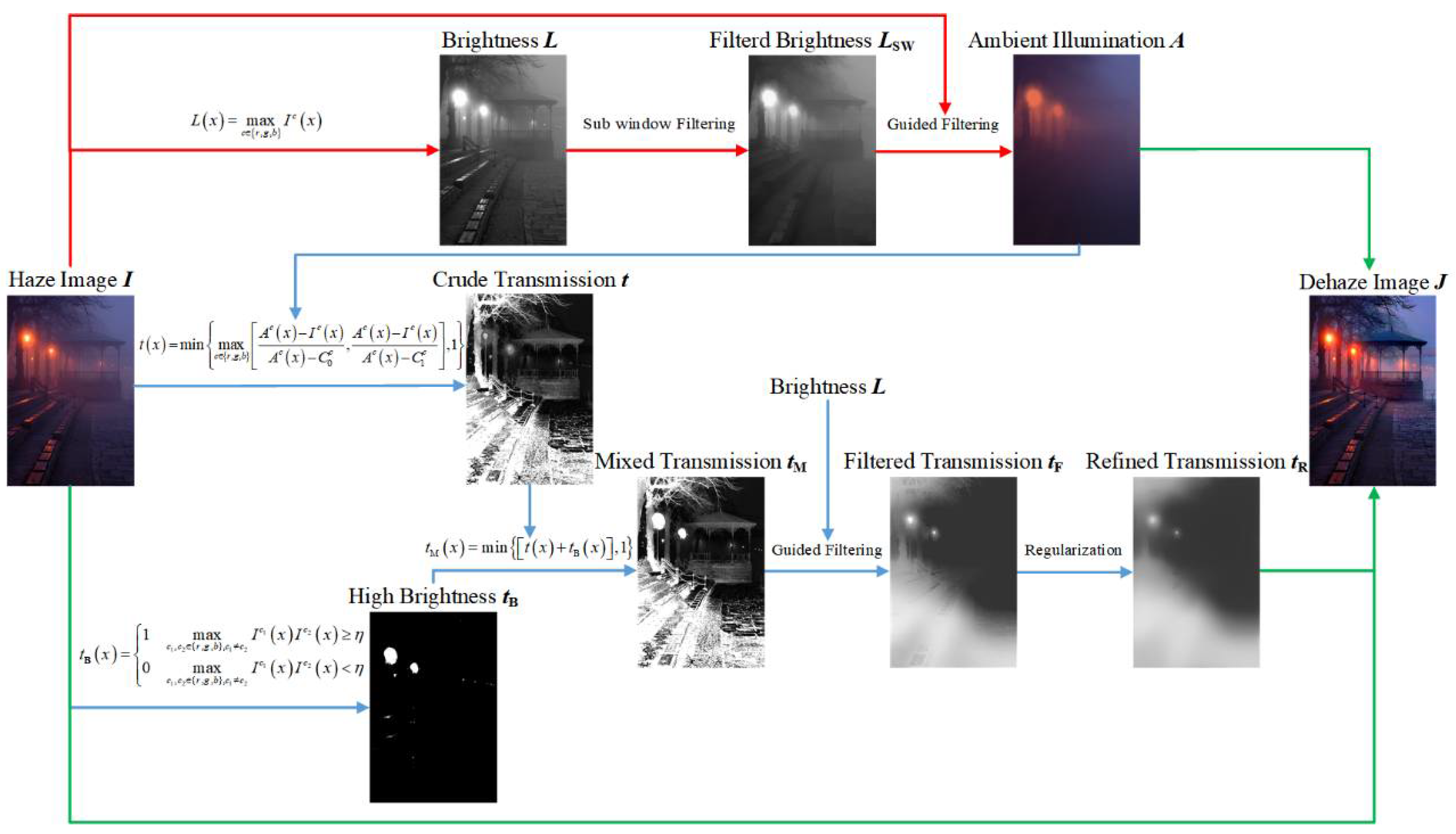
3. Proposed Dehazing Method

The flow chart of the proposed MF Dehazer is illustrated in Figure 1. The quality of the dehazing effect depends on the accuracy of the two parts of the estimation: the ambient illumination and the transmission. The detailed will follow.

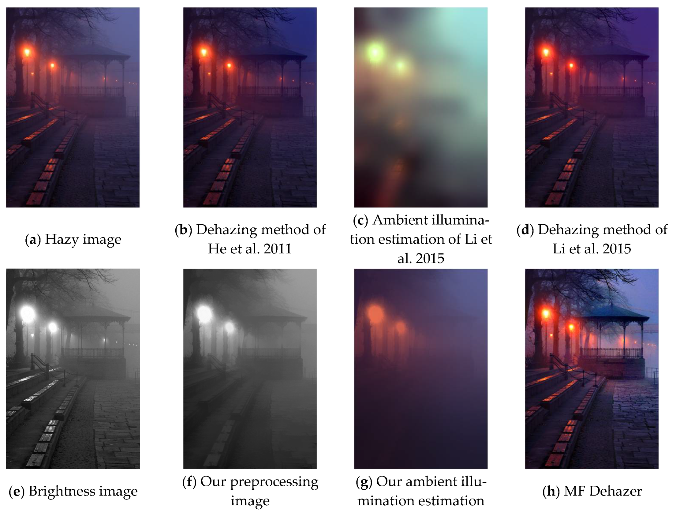
3.1. Mixed-Filter for Ambient Illumination Estimation

According to Retinex theory, we can Substitute (1) into (4):

$$I\left(x\right)=A\left(x\right)\left(R\left(x\right)t\left(x\right)+1-t\left(x\right)\right)$$

(5)

Ambient illumination, composed of the scattering and reflection of atmospheric light and artificial light sources is a spatially smooth and low-frequency term while $R\left(x\right)t\left(x\right)+1-t\left(x\right)$ serves as the high-frequency term. The traditional Retinex algorithm uses Gaussian filtering to estimate the low-frequency components. However, because Gaussian filtering does not retain the edge and it is isotropic, the shape of the light source and the direction of the light cannot be retained when the image is blurred, and the backlight area of the light source is also blurred. Considering this analysis, we propose to initially preserve the edge blur of the brightness of the hazy image. While retaining the shape of the light source and the direction of the light, filter the farther small light source and reflected light, and then pass it as the reference image to guide the filtering as the ambient illumination estimation.

We regard each target pixel as a potential edge and generate multiple local windows (called side windows) in the rectangular area around it. Each window aligns the target pixel with the edge or corner (rather than the center) of the window. In the discrete cases, define eight side windows: upper (U), lower (D), left (L), right ®, upper left (UL), upper right (UR), lower left (DL), and lower right (DR). The eight side windows are mean filtered with the original image, and the side window with the minimum Euclidean distance between the filtering result and the original image is selected as the optimal filtering side window of the target pixel. The process can be expressed as follows:

$$L_n=\frac{1}{N_n}{\displaystyle \sum }_{j\in {\mathsf{\omega }}_i^n}{\mathsf{\omega }}_{ij}{I}_j,N_n={\displaystyle \sum }_{j\in {\mathsf{\omega }}_i^n}{\mathsf{\omega }}_{ij} ,n\in S$$

(6)

where $L_n$ is the filter value of the sub-window, ${\mathsf{\omega }}_{ij}$ is the weight of the pixel $j$ near the target pixel $i$ based on the kernel function $F$ which is averaging; $I_j$ is the value of pixel $j$, and $S=U,D,L,R,UL,UR,DL,DR$ is the set of sub-window index.

After obtaining the filter values of the eight sub-windows, in order to preserve the edge information, we use the sub-window with the minimum Euclidean distance to the input intensity as the output of $L_{sw}$.

$$L_{sw}=arg\underset{n\in S}{\min }\parallel I_i-L_n{\parallel }_2^2$$

(7)

We assume that the guided image and the output ambient illumination are linear, and then the brightness filtered image $L_{sw}$ is used as the guide image to obtain the linear transform parameter by minimizing the cost function of the target image $I$:

$$\mathrm{E}\left(a_k,b_k\right)={\displaystyle \sum }_{x\in {\mathsf{\omega }}_k}\left({\left(a_k{L}_{sw}\left(x\right)+b_k-I\left(x\right)\right)}^2+\mathsf{\lambda }{a}_k^2\right)$$

(8)

where ${\mathsf{\omega }}_k$ is the filter window, $\mathsf{\lambda }$ is the regularization coefficient with a value of 0.01, which is mainly used to prevent the solution $a_k$ from being too large.

Solve (8) using the least square method as follows:

$$\{\begin{array}{c}{a}_k=\frac{\frac{1}{\left|\omega \right|}{{\displaystyle \sum }}_{i\in {\mathsf{\omega }}_k}{L}_{sw}{I}_i-{\mu }_k{I}_k}{{\mathsf{\sigma }}_k^2+\lambda }\\ b_k=I_k-a_k{\mathsf{\mu }}_k\end{array}$$

(9)

where ${\mathsf{\mu }}_k$ and ${\mathsf{\sigma }}_k^2$ are the mean and variance of $L_{sw}$ in window ${\mathsf{\omega }}_k$, $\left|\omega \right|$ is the number of pixels in the window; $I_k$ is the mean value of all elements in the filter ${\mathsf{\omega }}_k$. After obtaining the coefficients $a_k$ and $b_k$, the ambient illumination estimation $A^c\left(x\right)$ can be obtained by using the mean value of the window containing the pixels as follows:

$$A^{ }\left(x\right)=\frac{1}{\left|\omega \right|}{\displaystyle \sum }_{i\in {\mathsf{\omega }}_k}{a}_k{L}_{sw}\left(x\right)+b_k$$

(10)

Figure 2 shows the comparison of different ambient illumination estimation methods and dehazing effects. He et al.’s [9] method chooses the brightest pixels in the image as the fixed value of the ambient illumination, which is affected by nighttime artificial light sources. If the brightness of the artificial light source is used as the ambient illumination, the light estimation will be higher. As a result, the color of the dehazing image in Figure 2b is too dark, which verifies that the ambient illumination estimation for nighttime dehazing should be a local variable rather than a fixed value. Because of the occlusion, the nighttime ambient illumination is directional and not scattered around. At the same time, the illumination intensity will decrease sharply due to the increase in distance and reflection. Therefore, the reflected light and the distant light source as a low light source should reduce the impact of illuminance estimation. It can be seen from Figure 2a,e that this image light is mainly two red light sources and presents umbrella-shaped illumination on the upper left. The ambient illumination estimation method of Li et al. [26] changes the color of the original light source, and because of its inability to preserve the edge, the light erodes to the backlight side. In comparison, we use the preprocessing image obtained by sub-window filtering as the guide image for ambient illumination estimation. The proposed method retains these two characteristics, and the color after dehazing is closer to the original color.

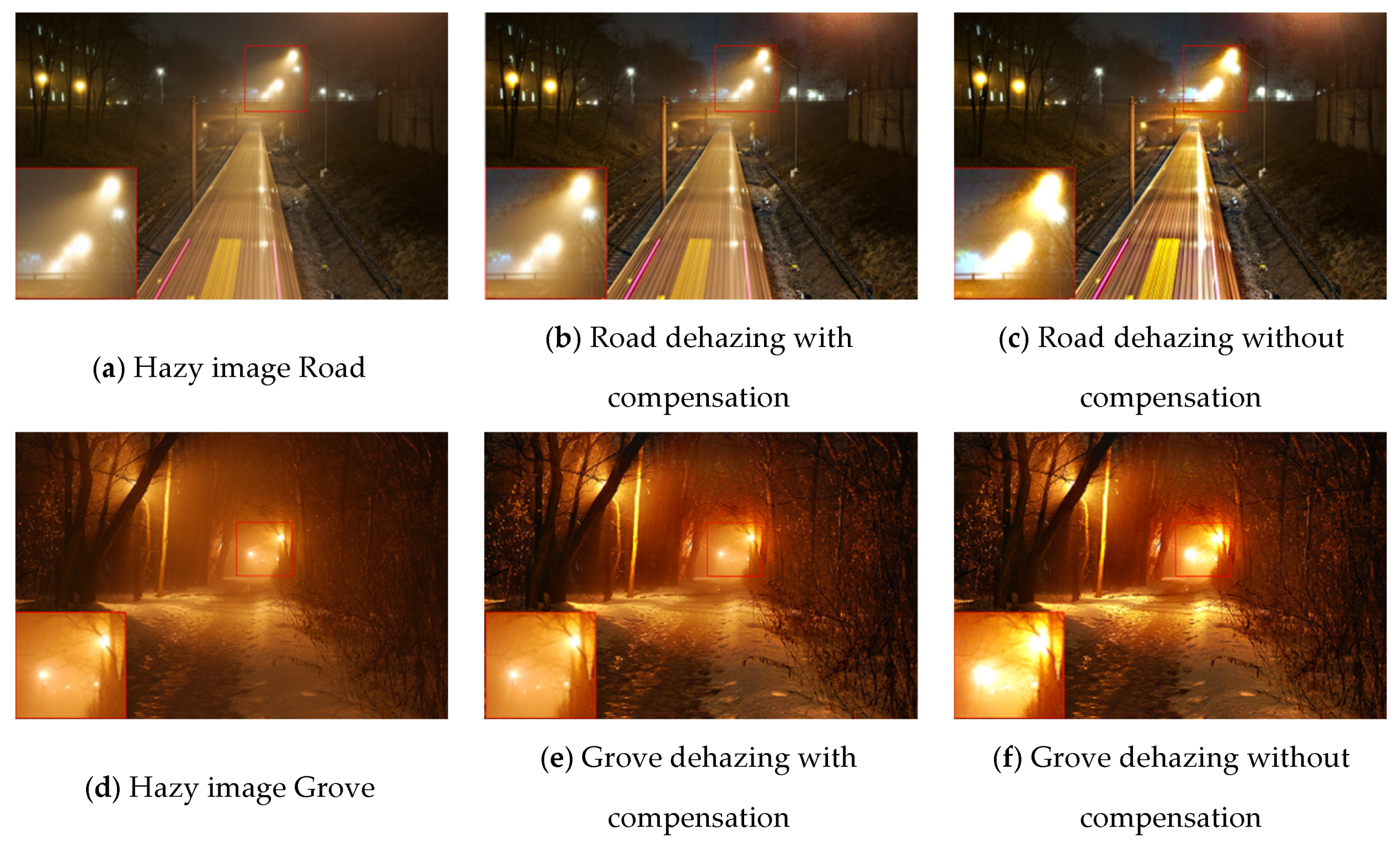
3.2. High-Light Area Transmission Compensation

Inspired by Meng et al. [14], we used boundary-constrained initial transmission estimation to replace the dark channel prior. The initial transmission obtained by this method can make the image more structured:

$$t\left(x\right)=\underset{ }{\min }\left\{\underset{c\in r,g,b}{\max }\left\{\frac{A^c\left(x\right)-I^c\left(x\right)}{A^c\left(x\right)-C_0^c} , \frac{A^c\left(x\right)-I^c\left(x\right)}{A^c\left(x\right)-C_1^c}\right\} ,1\right\}$$

(11)

where $C_0^c$ and $C_1^c$ are the upper and lower boundaries of the three channels.

After the nighttime haze image has been processed for dehazing, the problem of light source diffusion often occurs. It causes the light source to lose its original shape and boundary. This is because the transmission of the light source area is incorrectly estimated. We can draw a conclusion from (3) that with the increased transmission, the pixel value of the image after dehazing will decrease, and when the transmission is closer to 1, the dehazed image will be closer to the hazy image. Thus, the transmission affects the degree of image dehazing. The transmission of the light source area of these methods is estimated to be low, which causes the pixel value to increase after the dehazing of the light source area, and the phenomenon of diffusion occurs. Based on this, we propose high-light area transmission compensation for nighttime scenes to reduce the degree of the dehazing of the light source area to suppress the diffusion. At the same time, considering that the nighttime light sources are mostly colored light sources, at least one of the color channels has a very high value. So the maximum value of the two-channel product is selected as the basis for distinguishing whether it is the light source area as follows:

$$t_B\left(x\right)=\{\begin{array}{c}1 \underset{c_1,c_2\in r,g,b,c_1\ne c_2}{\max }{I}^{c_1}\left(x\right)I^{c_2}\left(x\right)\ge \eta \\ 0 \underset{c_1,c_2\in r,g,b,c_1\ne c_2}{\max }{I}^{c_1}\left(x\right)I^{c_2}\left(x\right)<\eta \end{array}$$

(12)

where $\eta$ is the threshold with a value of 0.3, which is used to distinguish whether the light source area is in this image, $c_1$ and $c_2$ represents two different color channels in the image, and $t_B$ is the compensation value.

After the transmission is compensated for the high-light area, in order to prevent it from exceeding the boundary, it is restricted using the following:

$$t_M\left(x\right)=\underset{ }{\min }\left\{\left(t\left(x\right)+t_B\left(x\right)\right),1\right\}$$

(13)

Finally, guided filtering is used to solve the problem of artifacts in the synthesized transmission after dehazing. Figure 3 shows the effect comparison of whether to use high-light area transmission compensation. This simple method improves the image quality of the light source area so that it retains the shape and boundary of the original light source.

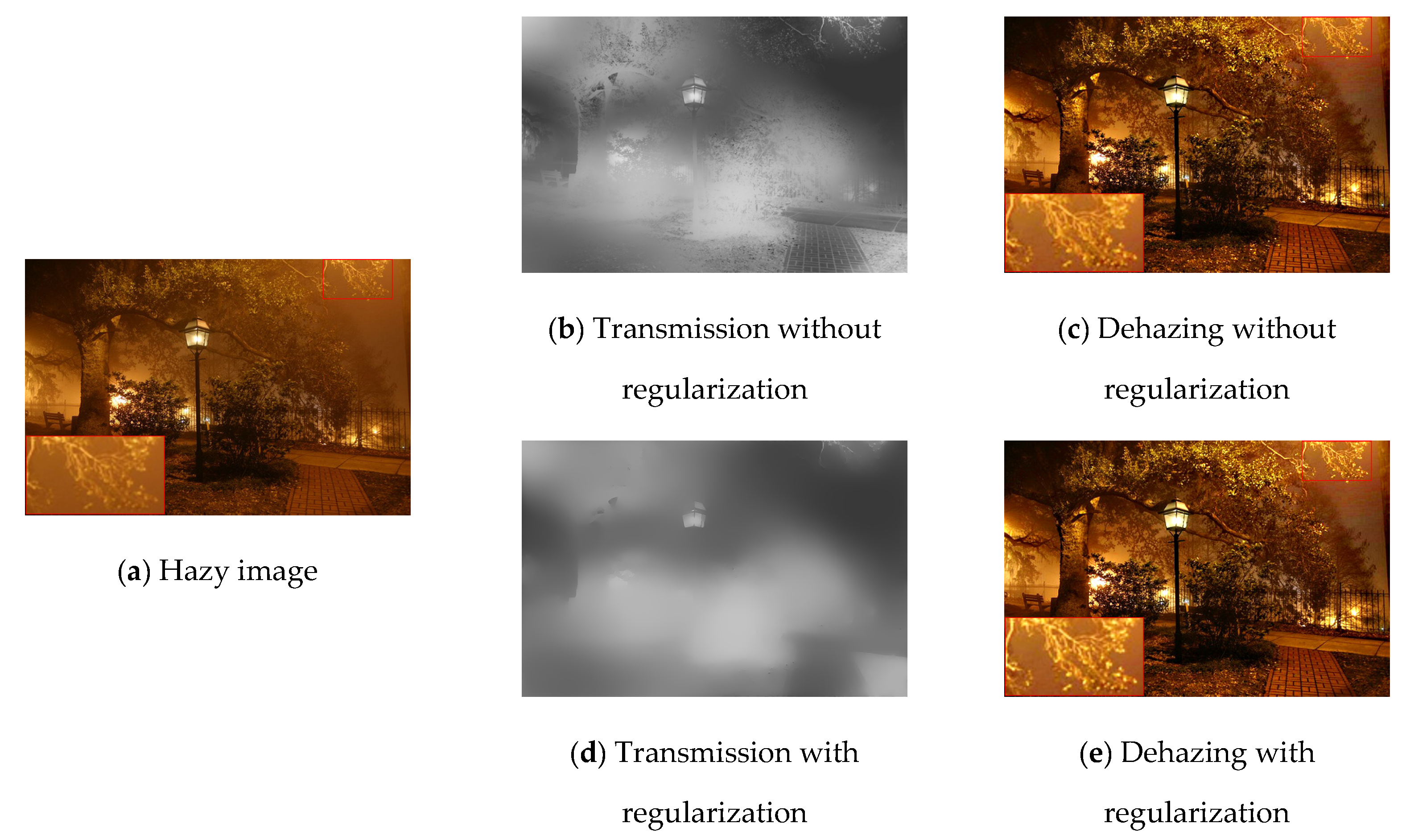
3.3. Regularization and Dehazing

With the purpose of improving the spatial correlation of image pixels to avoid problems such as haze residue or excessive dehazing, we used regularization to find the optimal transmission to improve the image quality. We used the L2-norm as the regularization term and as the data term to prevent over-fitting. We used the L1-norm, which is more robust to outliers, instead of the L2-norm so as to increase the depth of information sensitivity. We find the optimal transmission $t_R$ by minimizing the following objective function:

$$L={\displaystyle \sum }_x{\left(t_F\left(x\right)-t_R\left(x\right)\right)}^2+\lambda {\displaystyle \sum }_x{\displaystyle \sum }_{y\in N_x}w\left(x,y\right)\left|t_F\left(x\right)-t_F\left(y\right)\right|$$

(14)

where the first part is the data term that measures the fidelity by calculating the Euclidean distance between the transmission $t_F$ with the optimized transmission $t_R$. The second part is the regularization term, where $\mathsf{\lambda }$ is the regularization parameter. $N_x$ is the index set of the pixel $x$, and $w\left(x,y\right)$ is the weighting function. Here, we use the mixed function of color difference and brightness difference as seen in the following:

$$w\left(x,y\right)=\alpha ·exp\left(\frac{-\Vert c\left(x\right)-c{\left(y\right)\Vert }^2}{2{\sigma }^2}\right)+\left(1+\mathsf{\alpha }\right)\left({\left|l\left(x\right)-l\left(y\right)\right|}^{\beta }+\delta \right)$$

(15)

where $\alpha$ is the weight of the color difference and brightness difference, $c\left(x\right)$ and $c\left(y\right)$ are the color vectors, $\sigma$ is the prescribed parameter with the value of 0.5, $l\left(x\right)$ and $l\left(y\right)$ are the brightness vectors, $\beta$ is the brightness sensitivity parameter (typically 0.3) and $\delta$ is a small constant (typically 0.0001) to prevent this term from being 0.

After the optimized transmission is obtained by the least square method, the dehazing image can be obtained using (3). As shown in Figure 4, regularization can effectively improve the structure of image details.

4. Experimental Results and Discussion

To demonstrate the effectiveness of the proposed MF Dehazer in both day and night conditions, we conducted a series of experiments on the nighttime and daytime hazy images. The images used in the experiment are from the article [9,12,15]. The nighttime experiment and daytime experiment each used ten images of different resolutions. In the nighttime experiment, $\eta$ is 0.3, and the minimum transmission after guided filtering is 0.2. We compared MF Dehazer with recent nighttime dehazing methods [9,21,24,25,26]. In the daytime experiment, $\eta$ is 1 and the minimum transmission after guided filtering is 0.3. We compare MF Dehazer with recent daytime dehazing methods [9,12,14,15,21]. The comparison methods or pictures are provided by the authors.

4.1. Qualitative Comparison

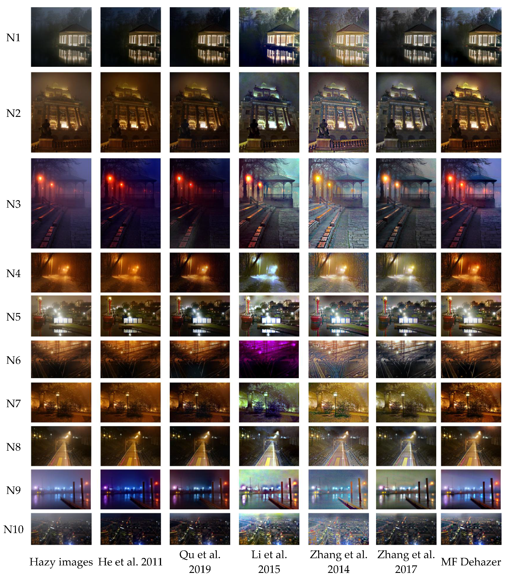
4.1.1. Nighttime Hazy Images

We chose the dark channel prior method of He et al. [9], the dehazing method based on deep learning of Qu et al. [21] and the recent nighttime dehazing methods of Li et al. [26], Zhang et al. [24] and Zhang et al. [25] to carry out the nighttime dehazing experiments. The experimental images are shown in Figure 5. He et al.’s [9] method incorrectly estimates the artificial light as the global ambient illumination, which causes the image to be too dark after dehazing. It proves that the nighttime ambient illumination should be a local variable rather than a simple fixed value. Because of the complex nighttime haze scene, the deep learning model of Qu et al. [21] cannot be effectively applied. It deepens the color of dim nighttime images and introduces unreal colors (Figure 5N3). Li et al.’s [26] method completely changes the color of the image, diffuses the light source, and the color is unstable (Figure 5N6,N9). Zhang et al.’s [24] method diffuses the image light in the light source area (Figure 5N1) and produces noise in the sky and dark areas (Figure 5N2,N3,N8,N10). Although Zhang et al.’s [25] method has better image clarity, it also cannot avoid the problem of noise (Figure 5N2,N3,N9) and light source area diffusion (Figure 5N3,N4). The proposed MF Dehazer effectively solves the defects of the above-mentioned methods. On the basis of retaining the original color, both the dark and bright areas of the image are effectively dehazed, such as the reflection of the lake in Figure 5N1, the clearer and more realistic green space on the left of Figure 5N10, the details and levels of shrubs and leaves in Figure 5N1,N3,N5,N7, and the light source diffusion problem of each image is well solved.

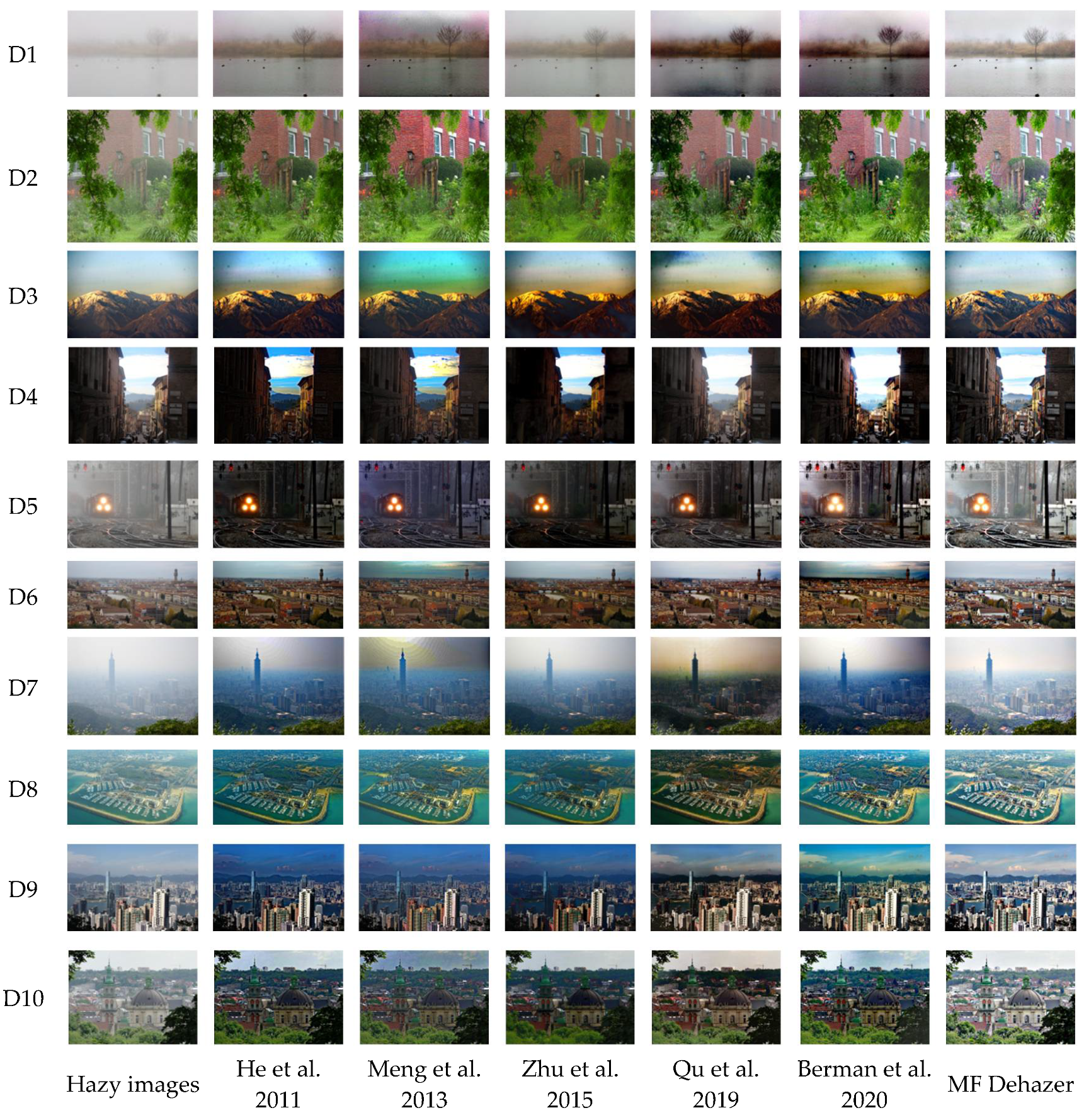
4.1.2. Daytime Hazy Images

We chose the different prior methods of He et al. [9], Meng et al. [14], and Zhu et al. [12], the dehazing method based on deep learning of Qu et al. [21] and the recent dehazing methods of Berman et al. [15] to carry out daytime dehazing experiments. When using He et al.’s [9] method, it is easy to overestimate the illumination, causing the image to be too dark (Figure 6D5), and one side is dark when there are far and near scenes (Figure 6D4,D8). Zhu et al.’s [12] method also has the same problem. Meng et al.’s [14] method does not handle the sky area well and produces noise (Figure 6D1,D6,D10) and color artifacts (Figure 6D7). Qu et al.’s [21] method in some areas of complex pictures, such as trees, deepens the color of the image and causes the details to be unrecognizable (Figure 6D7,D9,D10). Berman et al.’s [15] method produces color artifacts at the junction of the sky area. For example, the sky at the junction with the mountain turns yellow (Figure 6D3) or green (Figure 6D9) as it is affected by the color of the mountain. By contrast, MF Dehazer does not have these defects. The sky, lake and the near and far scenes are handled more naturally; the color is closer to the original image, and it looks visually pleasing.

4.2. Quantitative Comparison

Quantitatively,

Table 1. Comparosion Index of Nighttime Dehazing Effect.

Fig	Li et al. [26]			Zhang et al. [24]			Zhang et al. [25]			MF Dehazer
	SSIM	PSNR	CIEDE	SSIM	PSNR	CIEDE	SSIM	PSNR	CIEDE	SSIM	PSNR	CIEDE
N1	0.648	17.078	19.390	0.662	16.827	24.269	0.813	23.473	13.374	0.722	21.302	12.715
N2	0.785	22.409	20.535	0.604	16.792	24.755	0.853	24.581	19.095	0.875	23.336	9.879
N3	0.617	16.087	18.850	0.390	10.847	38.178	0.773	22.188	16.037	0.807	23.065	10.441
N4	0.835	20.538	24.970	0.509	12.383	31.265	0.802	17.728	19.609	0.862	27.378	8.717
N5	0.721	17.354	19.806	0.791	19.226	19.437	0.886	19.814	20.679	0.893	23.855	9.641
N6	0.505	15.928	38.064	0.464	12.897	34.054	0.856	22.522	16.096	0.850	26.994	6.379
N7	0.754	19.301	24.117	0.578	12.760	29.582	0.864	19.481	13.986	0.840	23.879	9.816
N8	0.789	20.211	15.214	0.557	14.504	29.129	0.919	24.864	13.196	0.937	28.517	5.432
N9	0.544	13.537	24.930	0.516	16.180	21.882	0.785	21.197	20.353	0.847	24.699	9.159
N10	0.624	14.883	21.399	0.488	12.455	32.707	0.812	22.313	15.336	0.770	20.74	14.063
AVG	0.682	17.733	22.727	0.556	14.487	28.526	0.836	21.816	16.776	0.840	24.382	9.624

and

Table 2. Comparision Index of Daytime Dehazing Effect.

Fig	He et al. [9]			Meng et al. [14]			Qu et al. [21]			Berman et al. [15]			MF Dehazer
	SSIM	PSNR	CIEDE	SSIM	PSNR	CIEDE	SSIM	PSNR	CIEDE	SSIM	PSNR	CIEDE	SSIM	PSNR	CIEDE
D1	0.814	13.271	18.816	0.504	8.828	35.924	0.750	9.465	31.349	0.494	8.951	33.463	0.764	21.993	5.157
D2	0.908	17.852	14.675	0.833	18.941	12.504	0.864	17.658	18.575	0.841	19.534	16.859	0.825	21.877	10.616
D3	0.769	16.842	23.342	0.869	16.160	31.645	0.746	15.974	23.298	0.788	15.956	22.663	0.841	24.477	9.325
D4	0.573	15.308	29.311	0.915	18.087	13.385	0.808	20.388	16.390	0.654	20.430	16.078	0.840	22.710	10.406
D5	0.390	8.001	69.811	0.677	10.590	47.519	0.638	10.650	45.258	0.514	11.511	39.448	0.680	18.441	13.277
D6	0.831	16.438	23.480	0.809	14.280	24.589	0.873	18.596	15.247	0.684	13.527	26.763	0.815	20.339	11.820
D7	0.783	11.012	40.420	0.762	10.053	41.852	0.675	9.198	41.730	0.713	10.267	44.883	0.858	24.290	6.633
D8	0.767	11.927	53.164	0.851	15.569	34.350	0.637	10.239	46.116	0.764	14.753	42.244	0.802	19.397	17.924
D9	0.746	11.884	50.448	0.845	13.223	38.019	0.784	13.746	30.346	0.825	16.084	37.390	0.811	18.061	17.161
D10	0.676	12.327	39.186	0.728	11.790	36.219	0.746	12.358	31.850	0.632	12.398	40.842	0.804	20.785	11.180
AVG	0.726	13.486	36.265	0.779	13.752	31.601	0.752	13.827	30.016	0.691	14.341	32.063	0.804	21.237	11.350

consider three well-known metrics: PSNR [29], SSIM and CIEDE2000 [30,31]. PSNR is the ratio of the maximum signal amount to the noise intensity, which measures the degree of image distortion. SSIM evaluates image quality from three aspects: brightness, contrast, and structure, which indicates the similarity of image structure information. Higher values indicate better quality for PSNR and SSIM. CIEDE2000 evaluates image quality from five aspects: brightness, chroma, hue, chroma difference, and hue difference, which indicates the chromatic aberration of the image. A lower value indicates better quality for CIEDE2000.

As shown in Table 1 and Table 2, whether it is nighttime or daytime, MF Dehazer is excellent in all metrics, especially in that the PSNR and CIEDE are much higher than in the other methods. It shows that the proposed method has less distortion after dehazing, can effectively reduce noise, and well retains the color of the original image. At the same time, the proposed MF Dehazer has high stability, and the various metrics do not fluctuate. It can adapt to hazy images of different environments and complexity and restore high-definition, high-contrast and high-structure dehazing images.

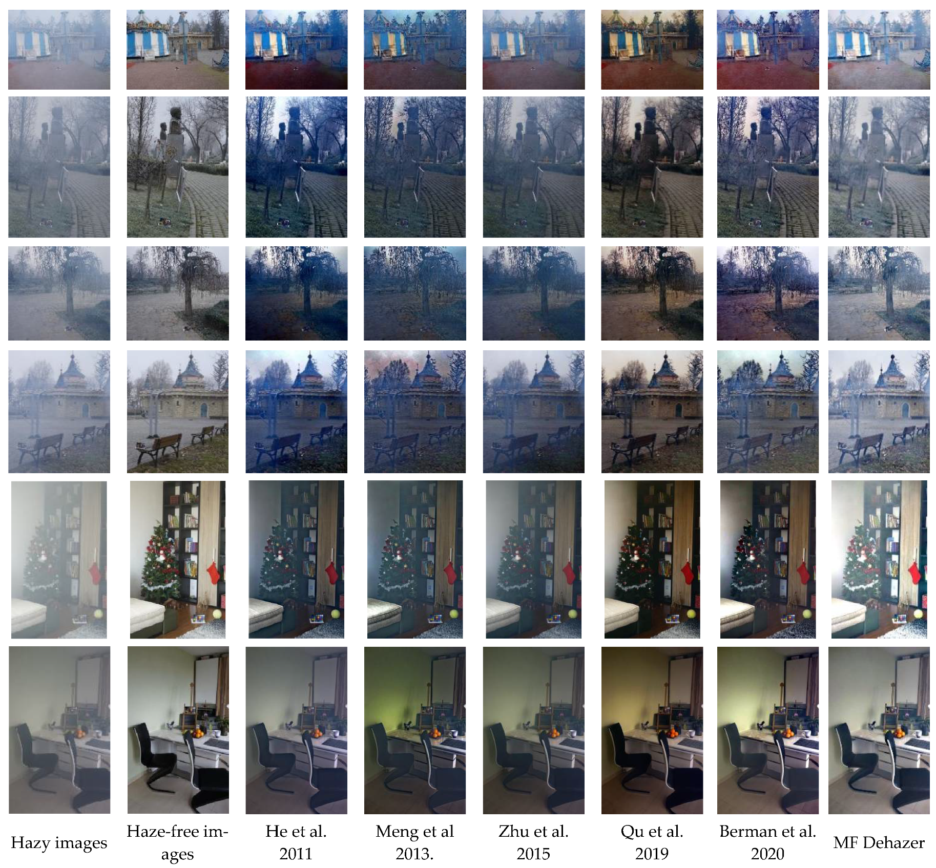
4.3. Real Haze-Free Image Comparison

Apart from the above experiments, we also tested 80 images from two public image datasets, O-HAZE and I-HAZE [32] for verification. These are dehazing benchmarks that include real hazy and haze-free images. Figure 7 shows a part of the experimental results, and

Table 3. Comparision Index Of O-Haze Additionally, I-HazeE.

Method	O-HAZE			I-HAZE
	SSIM	PSNR	CIEDE	SSIM	PSNR	CIEDE
He et al.	0.710	16.510	31.420	0.726	14.948	28.058
Meng et al.	0.727	17.379	25.351	0.746	14.345	26.156
Zhu et al.	0.619	17.103	24.220	0.708	15.391	26.316
Qu et al.	0.693	17.576	20.813	0.743	15.468	24.855
Berman et al.	0.722	16.544	24.027	0.762	15.713	23.132
MF Dehazer	0.770	17.272	20.231	0.792	16.135	20.958

shows the average objective indicators of these two datasets. Through the comparison in Figure 7, we can see that our results are close to the real haze-free image. At the same time, it confirms the advantages and disadvantages of the previous methods. All of the indicators in Table 3, except for the PSNR in O-HAZE, are higher than the existing methods. This indicator is lower than other methods because O-HAZE contains a lot of white dense fog scenes. When estimating the ambient illumination through the local filter window, the ambient illumination may be overestimated due to the influence of white dense haze, resulting in haze residue. Therefore, it is a defect of the proposed method to deal with the local white dense haze.

5. Conclusions

In this paper, we have proposed a dehazing method for the removal of haze from both nighttime and daytime images. For the ambient illumination estimation, we analyzed the visual properties of hazy images and preserved the illumination direction and shape of the original image using the mixed-filter method. In addition, for the transmission estimation, the proposed method solves the problem of light source diffusion and enhances the image’s sense of depth and definition. Both the qualitative and quantitative experimental results demonstrate that MF Dehazer is superior to the recent methods and provides a novel approach for obtaining a better quality dehazing image on the basis of preserving the original image color. However, much more work needs to be undertaken in the future. MF Dehazer shares this limitation because it uses a filter window to estimate the local ambient illumination. If the size of the local dense haze in the image is larger than the window size, it may overestimate ambient illumination and generate haze residue. The method will be improved to overcome these disadvantages.

References

1. Duan, J.; Liu, X. Online monitoring of green pellet size distribution in haze-degraded images based on VGG16-LU-net and haze judgement. IEEE Trans. Instrum. Meas. 2021, 70, 1–16. [Google Scholar] [CrossRef]
2. Zhang, J.; Lu, Z.; Li, M. Active Contour-Based Method for Finger-Vein Image Segmentation. IEEE Trans. Instrum. Meas. 2020, 69, 8656–8665. [Google Scholar] [CrossRef]
3. Xu, H.; Zhai, G.; Wu, X.; Yang, X. Generalized Equalization Model for Image Enhancement. IEEE Trans. Multimedia 2013, 16, 68–82. [Google Scholar] [CrossRef]
4. Land, E.H. The Retinex Theory of Color Vision. Sci. Am. 1977, 237, 108–128. [Google Scholar] [CrossRef] [PubMed]
5. Galdran, A.; Vazquez-Corral, J.; Pardo, D.; Bertalmío, M. Enhanced Variational Image Dehazing. SIAM J. Imaging Sci. 2015, 8, 1519–1546. [Google Scholar] [CrossRef] [Green Version]
6. Wang, Y.; Wang, H.; Yin, C.; Dai, M. Biologically inspired image enhancement based on Retinex. Neurocomputing 2016, 177, 373–384. [Google Scholar] [CrossRef]
7. Galdran, A.; Bria, A.; Alvarez-Gila, A.; Vazquez-Corral, J.; Bertalmio, M. On the Duality Between Retinex and Image Dehazing. In Proceedings of the 2018 IEEE/CVF Conference on Computer Vision and Pattern Recognition, Salt Lake City, UT, USA, 18–22 June 2018; pp. 8212–8221. [Google Scholar] [CrossRef] [Green Version]
8. Koschmieder, H. Theorie der horizontalen sichtweite. Beitrage zur Physik der Freien Atmosphare 1924, 12, 171–181. [Google Scholar]
9. He, K.; Sun, J.; Tang, X. Single Image Haze Removal Using Dark Channel Prior. IEEE Trans. Pattern Anal. Mach. Intell. 2010, 33, 2341–2353. [Google Scholar] [CrossRef] [PubMed]
10. He, K.; Sun, J.; Tang, X. Guided Image Filtering. IEEE Trans. Pattern Anal. Mach. Intell. 2013, 35, 1397–1409. [Google Scholar] [CrossRef] [PubMed]
11. Fattal, R. Single Image Dehazing. ACM Trans. Graph. 2008, 27, 1–9. [Google Scholar] [CrossRef]
12. Zhu, Q.; Mai, J.; Shao, L. A Fast Single Image Haze Removal Algorithm Using Color Attenuation Prior. IEEE Trans. Image Process. 2015, 24, 3522–3533. [Google Scholar] [CrossRef] [PubMed] [Green Version]
13. Berman, D.; Treibitz, T.; Avidan, S. Non-local Image Dehazing. In Proceedings of the 2016 IEEE Conference on Computer Vision and Pattern Recognition (CVPR), Las Vegas, NV, USA, 27–30 June 2016; pp. 1674–1682. [Google Scholar] [CrossRef]
14. Meng, G.; Wang, Y.; Duan, J.; Xiang, S.; Pan, C. Efficient Image Dehazing with Boundary Constraint and Contextual Regularization. In Proceedings of the ICCV—IEEE International Conference on Computer Vision, Sydney, Australia, 1–8 December 2013; pp. 617–624. [Google Scholar] [CrossRef]
15. Berman, D.; Treibitz, T.; Avidan, S. Single Image Dehazing Using Haze-Lines. IEEE Trans. Pattern Anal. Mach. Intell. 2018, 42, 720–734. [Google Scholar] [CrossRef] [PubMed]
16. Li, B.; Peng, X.; Wang, Z.; Xu, J.; Feng, D. AOD-Net: All-in-One Dehazing Network. In Proceedings of the 2017 IEEE International Conference on Computer Vision (ICCV), Venice, Italy, 22–29 October 2017; pp. 4780–4788. [Google Scholar] [CrossRef]
17. Chen, D.; He, M.; Fan, Q.; Liao, J.; Zhang, L.; Hou, D.; Yuan, L.; Hua, G. Gated Context Aggregation Network for Image Dehazing and Deraining. In Proceedings of the 2019 IEEE Winter Conference on Applications of Computer Vision (WACV), Waikoloa, HI, USA, 7–11 January 2019; pp. 1375–1383. [Google Scholar] [CrossRef] [Green Version]
18. Dong, J.; Pan, J. Physics-Based Feature Dehazing Networks. In Proceedings of the Computer Vision—ECCV 2020, Glasgow, UK, 23–28 August 2020; pp. 188–204. [Google Scholar]
19. Shao, Y.; Li, L.; Ren, W.; Gao, C.; Sang, N. Domain Adaptation for Image Dehazing. In Proceedings of the 2020 IEEE/CVF Conference on Computer Vision and Pattern Recognition (CVPR), Seattle, WA, USA, 13–19 June 2020; pp. 2805–2814. [Google Scholar] [CrossRef]
20. Dong, H.; Pan, J.; Xiang, L.; Hu, Z.; Zhang, X.; Wang, F.; Yang, M.-H. Multi-Scale Boosted Dehazing Network With Dense Feature Fusion. In Proceedings of the 2020 IEEE/CVF Conference on Computer Vision and Pattern Recognition (CVPR), Seattle, WA, USA, 13–19 June 2020; pp. 2154–2164. [Google Scholar] [CrossRef]
21. Qu, Y.; Chen, Y.; Huang, J.; Xie, Y. Enhanced Pix2pix Dehazing Network. In Proceedings of the 2019 IEEE/CVF Conference on Computer Vision and Pattern Recognition (CVPR), Long Beach, CA, USA, 15–20 June 2019; pp. 8152–8160. [Google Scholar] [CrossRef]
22. Deng, Q.; Huang, Z.; Tsai, C.-C.; Lin, C.-W. HardGAN: A Haze-Aware Representation Distillation GAN for Single Image Dehazing. In Proceedings of the Computer Vision—ECCV 2020, Glasgow, UK, 23–28 August 2020; pp. 722–738. [Google Scholar]
23. Pei, S.-C.; Lee, T.-Y. Nighttime haze removal using color transfer pre-processing and Dark Channel Prior. In Proceedings of the 2012 19th IEEE International Conference on Image Processing, Orlando, FL, USA, 30 September–3 October 2012; pp. 957–960. [Google Scholar] [CrossRef]
24. Zhang, J.; Cao, Y.; Fang, S.; Kang, Y.; Chen, C.W. Fast Haze Removal for Nighttime Image Using Maximum Reflectance Prior. In Proceedings of the 2014 IEEE International Conference on Image Processing (ICIP), Paris, France, 27–30 October 2014; pp. 4557–4561. [Google Scholar] [CrossRef]
25. Zhang, J.; Cao, Y.; Fang, S.; Kang, Y.; Chen, C.W. Fast Haze Removal for Nighttime Image Using Maximum Reflectance Prior. In Proceedings of the 2017 IEEE Conference on Computer Vision and Pattern Recognition (CVPR), Honolulu, HI, USA, 21–26 July 2017; pp. 7016–7024. [Google Scholar] [CrossRef]
26. Li, Y.; Tan, R.T.; Brown, M.S. Nighttime Haze Removal with Glow and Multiple Light Colors. In Proceedings of the 2015 IEEE International Conference on Computer Vision (ICCV), Santiago, Chile, 7–13 December 2015; pp. 226–234. [Google Scholar] [CrossRef]
27. CAncuti, C.; Ancuti, C.O.; De Vleeschouwer, C.; Bovik, A.C. Day and Night-Time Dehazing by Local Airlight Estimation. IEEE Trans. Image Process. 2020, 29, 6264–6275. [Google Scholar] [CrossRef] [PubMed]
28. Zhu, Z.; Wei, H.; Hu, G.; Li, Y.; Qi, G.; Mazur, N. A Novel Fast Single Image Dehazing Algorithm Based on Artificial Multiexposure Image Fusion. IEEE Trans. Instrum. Meas. 2020, 70, 1–23. [Google Scholar] [CrossRef]
29. Wang, Z.; Bovik, A.; Sheikh, H.; Simoncelli, E. Image Quality Assessment: From Error Visibility to Structural Similarity. IEEE Trans. Image Process. 2004, 13, 600–612. [Google Scholar] [CrossRef] [PubMed] [Green Version]
30. Sharma, G.; Wu, W.; Dalal, E.N. The CIEDE2000 color-difference formula: Implementation notes, supplementary test data, and mathematical observations. Color Res. Appl. 2005, 30, 21–30. [Google Scholar] [CrossRef]
31. Westland, S.; Ripamonti, C.; Cheung, V. Computational Colour Science Using MATLAB, 2nd ed.; Wiley: Hoboken, NJ, USA, 2012. [Google Scholar]
32. Ancuti, C.O.; Ancuti, C.; Timofte, R.; de Vleeschouwer, C. O-HAZE: A Dehazing Benchmark with Real Hazy and Haze-Free Outdoor Images. In Proceedings of the 2018 IEEE/CVF Conference on Computer Vision and Pattern Recognition Workshops (CVPRW), Salt Lake City, UT, USA, 18–22 June 2018; pp. 867–8678. [Google Scholar] [CrossRef]
Figure 1. Flow chart of the proposed dehazing method. In this chart, the red line is the ambient illumination estimation method, the blue line is the transmission estimation method, and the green line is the result.
Applsci 13 00255 g001
Figure 2. Comparison of ambient light estimation and dehazing by different methods. In order to ensure a fair comparison, we use the ambient illumination estimation methods of He et al. [9], Li et al. [26] and MF Dehazer and use the proposed transmission estimation method to remove haze to compare the effects of different ambient illumination estimation methods.
Applsci 13 00255 g002
Figure 3. Comparison of the high-light compensation effects.
Applsci 13 00255 g003
Figure 4. Comparison of regularizan.
Applsci 13 00255 g004
Figure 5. Comparison of nighttime dehazing [9,21,24,25,26].
Applsci 13 00255 g005
Figure 6. Comparison of daytime dehazing [9,12,14,15,21].
Applsci 13 00255 g006
Figure 7. Comparison of O-HAZE and I-HAZE [9,12,14,15,21].
Applsci 13 00255 g007