Article

Variable Step Block Hybrid Method for Stiff Chemical Kinetics Problems

1
Department of Fundamental and Applied Sciences, Faculty of Science and Information Technology, Universiti Teknologi PETRONAS, Seri Iskandar 32610, Perak, Malaysia
2
Department of Mathematics, Faculty of Natural Sciences, University of Jos, Jos 930003, Nigeria
3
Centre for Foundation Studies, Universiti Teknologi PETRONAS, Seri Iskandar 32610, Perak, Malaysia
4
Department of Information System, Universitas Islam Indragiri, Tembilahan 29281, Indonesia
5
Department of Food Science, Universitas Islam Indragiri, Tembilahan 29281, Indonesia
6
Department of Informatics Engineering, Faculty of Engineering, Universitas Islam Riau, Tembilahan 28284, Indonesia
*
Authors to whom correspondence should be addressed.
Appl. Sci. 2022, 12(9), 4484; https://doi.org/10.3390/app12094484
Submission received: 6 April 2022 / Revised: 25 April 2022 / Accepted: 26 April 2022 / Published: 28 April 2022
(This article belongs to the Topic Engineering Mathematics)

Abstract

:
Integration of a larger stiff system of initial value problems emerging from chemical kinetics models requires a method that is both efficient and accurate, with a large absolute stability region. To determine the solutions of the stiff chemical kinetics ordinary differential equations that help in explaining chemically reactive flows, a numerical integration methodology known as the 3-point variable step block hybrid method has been devised. An appropriate time step is automatically chosen to give accurate results. To check the efficiency of the new method, the numerical integration of a few renowned stiff chemical problems is evaluated such as Belousov–Zhabotinskii reaction and Hires, which are widely used in numerical studies. The results generated are then compared with the MATLAB stiff solver, ode15s.

1. Introduction

Stiff chemical kinetic models are required for the modeling of a practically real-world chemical system, such as atmospheric chemistry, energy conversion and storage, chemical engineering, the environment and materials, and biomedical and pharmaceutical engineering [1,2,3].
The following Ordinary Differential Equations (ODEs) can be used to model a homogeneous chemical reaction system:
y = f ( t , y ) ,       t 0 t t f i n a l
y ( t 0 ) = y 0
The column vector of species concentration is represented by y = [ y 1 , y 2 , ,   y N ] T   and N represents the total quantity of chemical species where t denotes the time, and the initial and final time are symbolized as t 0 and t f i n a l , respectively. The initial species concentrations are indicated by the column vector y 0 . Numerical solutions for stiff ODE systems defined by Equation (1) can be obtained using explicit or implicit ODE integrator [4,5,6,7,8]. Many ODEs have been used for chemical kinetic models; however, they are stiff [9], and solving stiff ODEs using an explicit technique necessitates very short time steps, making integration computationally intensive. Alternatively, implicit ODE integrators, such as the Backward Differentiation Formula (BDF), can be employed. In general, the implicit methods usually involve Newton Iteration for solving stiff systems of ODEs which is time-consuming because it consists of a Jacobian matrix that needs to be solved for every integration step. Therefore, it is still a research focus to deal with the Jacobian part for solving stiff system of ODEs [10,11], which is a fundamental aspect of several reaction-diffusion systems, such as in energy conversion, medicinal applications, and chemical engineering.
Although it is intricate to provide a clear description of the stiffness of the chemical kinetic model, one of the conditions can be if different species have significantly different time scales. Some fast-evolving organisms, for example, have very small time scales, whereas others evolve slowly and take longer time scales. The computing cost of explicit ODE integrators created for non-stiff problems against implicit ones, developed for stiff problems on the application is a realistic way to quantify stiffness. The problem can also be classified as very stiff if the computational cost of using an implicit ODE integrator is significantly less than the cost of an explicit ODE integrator [12].
The backward differentiation formula (BDF), often known as Gear’s approach and initially proposed in [13], is the foundation for many well-known strategies for addressing stiff problems. Various researchers, such as [1,14,15,16,17], proposed methods to increase the accuracy and computation time for stiff problems. Ref. [17] presented the idea of using the Block Backward Differentiation Formula (BBDF) to solve first-order stiff problems and since then the BBDF approach is increasingly being used to solve stiff ODEs. There are many solvers based on the BBDF method that are used to solve stiff ODEs that have been developed in the literature [18,19,20].
BDF has been extensively used because of its high stability properties. Based on the classical BDF method, several block methods have been proposed. The BBDF is one of the most prominent block approaches based on BDFs ([20,21,22]). r –point Block Backward Differentiation Formula ( r –BBDF) presented by [23], are used and expanded later. The block method based on BDF is particularly efficient for solving stiff ODEs to reduce the computational time and enhance the accuracy [24,25].
Despite having many advantages, the block method has the major drawback that the order of interpolation points could not surpass the order of differential equations [26,27]. As a result of this drawback, the addition of off-step points in the block was introduced and named the Hybrid method. Hybrid block approaches for the solution of IVPs in ODEs were proposed by [28,29,30]. Although this method is difficult to implement, it provides a better approximation than the k step method, specifically when the step length is shorter. The developed methods provided improved stability properties and circumvented the Dahlquist stability constraint by introducing off-step points [31]. Hybrid methods have also demonstrated improved stability, particularly when the problem is stiff or oscillatory [32,33].
Motivated by the above literature reviews, this study is aimed to develop a 3–point variable step block hybrid method (3–point VSBHM), by applying Lagrange polynomials as the basis function. In addition, the variable step–BBDF with an increment of step sizes to a factor of 1.6 and 1.9 has been studied by [17,34]. The proposed method will be employed on stiff chemical kinetics modeling as shown in Equation (1). For the purpose of selecting off–step points, several points have been observed and hence it is found that when the step size of the off–step point is halved, the 3-point VSBHM is zero stable. The proposed method has the advantage of the solutions being approximated at three points simultaneously when compared with MATLAB stiff solver ode15s.
The organization of the paper is as follows; Section 2 briefly describes the formulation of the method. Section 3 comprises of stability analysis of 3–point VSBHM with its properties. Section 4 elaborates on the implementation of the derived method followed by the step size strategy. A list of tested problems is presented in Section 5. Section 6 contains results and a discussion of the tested problems. Finally, Section 7 is the conclusion.

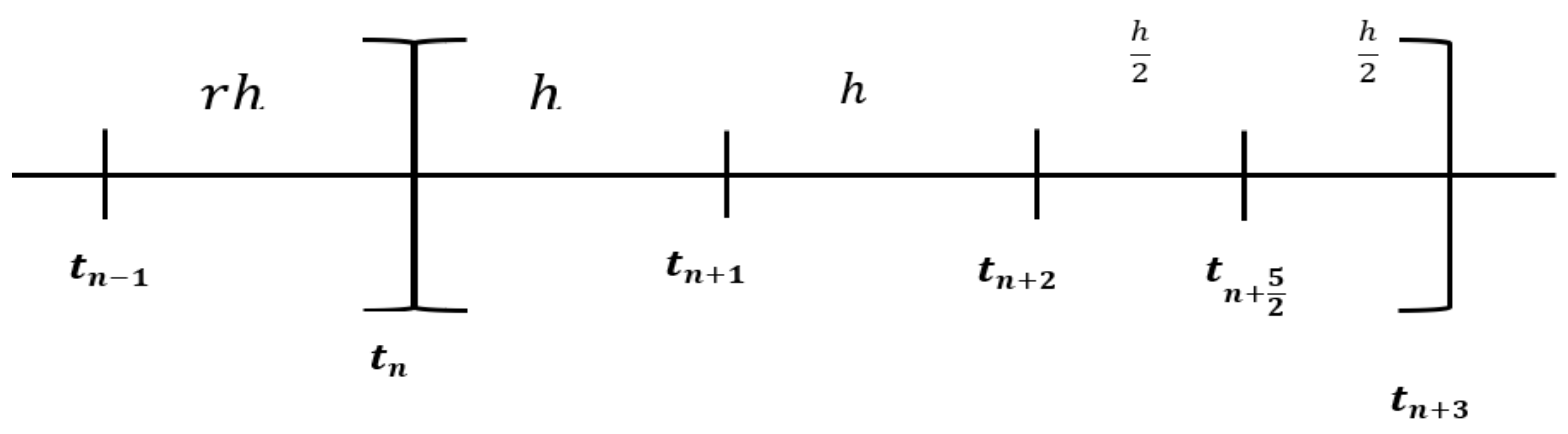
2. Formulation of 3–Point Variable Step Block Hybrid Method (3–Point VSBHM)

This section discusses the formulation of 3–point VSBHM. The three values of y n + 1 , y n + 2 , and y n + 3 with one off-step point y n + 5 2 are calculated concurrently in a block using earlier blocks with each block containing three points (refer to Figure 1). The computed block contains 3 h as the step size and r h   pointed out the previous block where r shows the step size ratio. To manage the step size, the step size ratio ( r ), is considered throughout the derivation process. The values of r   used in [17] were r = 1 , 2 , 5 8 even though r = 1 ,   2 ,     10 19 used in [5]. Hence, values r = 1 , r = 2 and r = 10 19 are considered in this research as the strategy to maintain, halve, or increase the step size by a factor of 1.9, respectively.
The interpolating polynomial P k ( t ) interpolates the values of a function f ( t , y ) in Equation (1) at k = 6 with interpolating points of ( t n 1 , y n 1 ), (   t n , y n ), (   t n + 1 , y n + 1 ), (   t n + 2 , y n + 2 ), (   t n + 5 2 , y n + 5 2 ) and ( t n + 3 , y n + 3 ). Lagrange polynomial P k ( t ) is defined as:
P k ( t ) = L k , 5 / 2 ( t ) y ( t n + 5 / 2 ) + j = 0 k 2 L k , j ( t ) y ( t n + 3 j )
where
L k , j ( t ) = ( i = 0 i j t t n + 3 i t n + 3 j t n + 3 i ) ( t t n + 5 2 t n + 3 j t n + 5 2 )   for   each   j = 0 , 1 , , k 2 , and   L k , 5 / 2 ( t ) = i = 0 k 2 t t n + 3 i t n + 5 / 2 t n + 3 i .
Let s = t t n + 1 h and replace y ( t )   in Equation (1) by a polynomial Equation (3). To obtain the y ,   the resultant polynomial in Equation (3) is differentiated for s at point t and substitute d t by h d s , so that
y = f ( t , y )
h P k ( t n + 1 + s h )   =   y n + 3 3 ( 3 + r ) [ 1 2 ( 3 + 2 s 15 s 2 4 s 3 + 10 s 4 + r ( 3 4 s 9 s 2 + 8 s 3 ) ) ] 32 y n + 5 2 15 ( 5 + 2 r ) [ 5 s 4 4 s 3 9 s 2 + 2 s + 2 + r ( 4 s 3 6 s 2 2 s + 2 ) ] + y n + 2 ( 2 + r ) [ 3 + 5 s 9 s 2 6 s 3 + 5 s 4 + r ( 3 s 15 s 2 2 + 4 s 3 ) ] y n + 1 3 ( 1 + r ) [ 1 2 ( 1 + 22 s 9 s 2 20 s 3 + 10 s 4 ) + r ( 7 + 8 s 21 s 2 + 8 s 3 ) ] + y n 15 r [ 3 + 7 s + 6 s 2 14 s 3 + 5 s 4 + r ( 3 + 13 s 22 s 2 2 + 4 s 3 ) ] y n 1 r ( r + 1 ) ( r + 2 ) ( r + 5 2 ) ( r + 3 ) [ 3 + 7 s + 6 s 2 14 s 3 + 5 s 4 ]
By substituting s = 0 ,   1 ,   3 2   and 2 into Equation (4) we obtain,
h f ( t n + 1 ) = ( 1 + r ) 2 ( 3 + r ) y n + 3 64 ( 1 + r ) 15 ( 5 + 2 r ) y n + 5 2 + 3 ( 1 + r ) 2 + r y n + 2 ( 1 + 7 r ) 6 ( 1 + r ) y n + 1 3 ( 1 + r ) 15 r y n + 3 y n 1 r ( r + 1 ) ( r + 2 ) ( r + 5 2 ) ( r + 3 )
h f ( t n + 2 ) = ( r 2 ) 3 ( 3 + r ) y n + 3 + 64 ( 2 + r ) 15 ( 5 + 2 r ) y n + 5 2 ( 3 r + 4 ) 2 ( 2 + r ) y n + 2 ( 2 + r ) 3 ( 1 + r ) y n + 1 + ( 2 + r ) 30 r y n 1 r ( r + 1 ) ( r + 2 ) ( r + 5 2 ) ( r + 3 ) y n 1
h f ( t n + 5 2 ) = ( 75 + 30 r ) 48 ( 3 + r ) y n + 3 + 2 ( 55 + 16 r ) 15 ( 5 + 2 r ) y n + 5 2 ( 75 + 30 r ) 16 ( 2 + r ) y n + 2 ( 25 + 10 r ) 48 ( 1 + r ) y n + 1 ( 15 + 6 r ) 240 r y n 15 16 ( r + 1 ) ( r + 2 ) ( r + 5 2 ) ( r + 3 ) y n 1
h f ( t ) = ( 75 + 23 r ) 3 ( 3 + r ) y n + 3 32 ( 18 + 6 r ) 15 ( 5 + 2 r ) y n + 5 2 + ( 9 + 3 r ) 2 + r y n + 2 ( 9 + 3 r ) 6 ( 1 + r ) y n + 1 + ( 3 + r ) 15 r y n 3 r ( r + 1 ) ( r + 2 ) ( r + 5 2 ) ( r + 3 ) y n 1
On substituting r = 1 , r = 2 and r = 10 19   into Equations (5)–(8) gives the coefficients for 3-point VSBHM are presented as in Table 1. These r values are properly considered for zero stability and computational efficiency.

3. Stability Analysis of 3–Point VSBHM with Its Properties

The practical significance of a method is dependent on its region of absolute stability that ensures solving at least slightly stiff problems [35]. The stability properties of the proposed methods are examined in this section to illustrate their use in resolving stiff problems. For a method to be stable, some definitions will be provided to support the practical criterion in addressing stiff problems.

3.1. Zero-Stability

Definition 1. (Zero-stable).
“The Linear Multistep Method (LMM) is said to be zero-stable if no root of the first characteristic polynomial, p ( t )   has modulus greater than one, and if every root with modulus one is simple”.
Definition 2. (A-stable).
“A method is said to be A-stable if all numerical approximations tend to zero when it is applied to the differential equation y = λ y with a fixed positive h   and a complex constant λ with negative real part”.
Ref. [36] proposed the scalar test to determine the stability of the method for Table 1 as
y = λ y ,   λ   <   0 ,
where λ represents the complex constant with Re(λ) < 0. Equation (9) is substituted in Table 1, therefore it precedes for r = 1 as,
y n + 1 = 3 56 y n 1 3 5 y n + 3 y n + 2 64 35 y n + 5 2 + 3 8 y n + 3 3 2 h λ y n + 1 y n + 2 = 1 98 y n 1 + 3 35 y n 3 7 y n + 1 + 384 245 y n + 5 2 3 14 y n + 3 6 7 h λ y n + 2 y n + 5 2 = 75 9088 y n 1 + 147 2272 y n 1225 4544 y n + 1 + 3675 2272 y n + 2 3675 9088 y n + 3 + 105 142 h λ y n + 5 2 y n + 3 = 3 343 y n 1 16 245 y n + 12 49 y n + 1 48 49 y n + 2 + 3072 1715 y n + 5 2 + 12 49 h λ y n + 3
Equation (10) is then inscribed into the matrix form to attain the matrix as follows
3 8 64 35 3 1 + 3 2 h λ 3 14 384 245 1 + 6 7 h λ 3 7 3675 9088 1 105 142 h λ 3675 2272 1225 4544 1 12 49 h λ 3072 1715 48 49 12 49 y n + 3 y n + 5 2 y n + 2 y n + 1 = 3 5 0 3 56 0 3 35 0 1 98 0 147 2272 0 75 9088 0 16 245 0 3 343 0 y n y n 1 2 y n 1 y n 2
whereas,
which is equivalent to,
C = [ 3 8 64 35 3 1 + 3 2 h λ 3 14 384 245 1 + 6 7 h λ 3 7 3675 9088 1 105 142 h λ 3675 2272 1225 4544 1 12 49 h λ 3072 1715 48 49 12 49 ] ,   D = [ 3 5 0 3 56 0 3 35 0 1 98 0 147 2272 0 75 9088 0 16 245 0 3 343 0 ]
C Y N = D Y N 1 ,
where C and D in Equation (11) are appropriately selected m × m matrix coefficients and N represent the number of blocks (note that the evaluation presented here is only for r = 1. For (r = 2, 10/19), the same procedure is considered). H = h λ is replaced in the matrices which are obtained by Equation (10). The stability polynomials R r ( t , H ) correlated with Table 1 are attained by solving the characteristic equations | C t D | using different step size ratios ( r = 1 ,   2 , 10 19 ) .
R 1 ( t , H ) = 9 t 2 48 , 706 + 27 H t 2 97 , 412 + 9 H 2 t 2 97 , 412 23 , 076 t 3 24 , 353 24 , 462 H t 3 24 , 353 9279 H 2 t 3 24 , 353 2889 H 3 t 3 48 , 706 + 41 , 616 t 4 48 , 706 179 , 199 H t 4 97 , 412 + 159 , 417 H 2 t 4 97 , 412 40 , 851 H 3 t 4 48 , 706 + 810 H 4 t 4 3479
R 2 ( t , H ) = 2 t 2 87 , 725 + 3 H t 2 87 , 725 + H 2 t 2 87 , 725 49 , 614 t 3 87 , 725 47 , 203 H t 3 87 , 725 16 , 897 H 2 t 3 87 , 725 534 H 3 t 3 17 , 545 + 49 , 616 t 4 87 , 725 20 , 104 H t 4 17 , 545 + 94 , 716 H 2 t 4 87 , 725 954 H 3 t 4 1595 + 648 H 4 t 4 3509
R 10 / 19 t , H = 44 , 569 , 782 t 2 47 , 034 , 975 , 875 + 66 , 854 , 673 H t 2 47 , 034 , 975 , 875 + 22 , 284 , 891   H 2 t 2 47 , 034 , 975 , 875 74 , 668 , 516 , 218 t 3 47 , 034 , 975 , 875 97 , 422 , 580 , 953 H t 3 47 , 034 , 975 , 875 40 , 170 , 428 , 271   H 2 t 3 47 , 034 , 975 , 875 231 , 953 , 814 H 3 t 3 1 , 881 , 399 , 035 + 597 , 704 , 688   t 4 376 , 279 , 807 5 , 555 , 509 , 848   H t 4 1 , 881 , 399 , 035 + 4 , 692 , 538 , 692 H 2 t 4 1 , 881 , 399 , 035 2 , 257 , 808 , 634 H 3 t 4 1 , 881 , 399 , 035 + 115 , 833 , 888 H 4 t 4 376 , 279 , 807
The zero stability is determined from the stability polynomial in Equations (12)–(14) by substituting H = h λ = 0 into Equations (12)–(14), generating
R 1 ( t , H ) = 9 t 2 48 , 706 23 , 076 t 3 24 , 353 + 41 , 616 t 4 48 , 706
R 2 ( t , H ) = 2 t 2 87 , 725 49 , 614 t 3 87 , 725 + 49 , 616 t 4 87 , 725
R 10 / 19 ( t , H ) = 44 , 569 , 782   t 2 47 , 034 , 975 , 875 74 , 668 , 516 , 218   t 3 47 , 034 , 975 , 875 + 597 , 704 , 688 t 4 376 , 279 , 807
By equating Equations (15)–(17) = 0 , the roots of stability polynomial can be obtained. Table 2 presents the roots for variable step sizes.
Since all the roots lie within |t| ≤ 1 described in Definition 1, hence, the method 3–point VSBHM is determined as a zero stable.

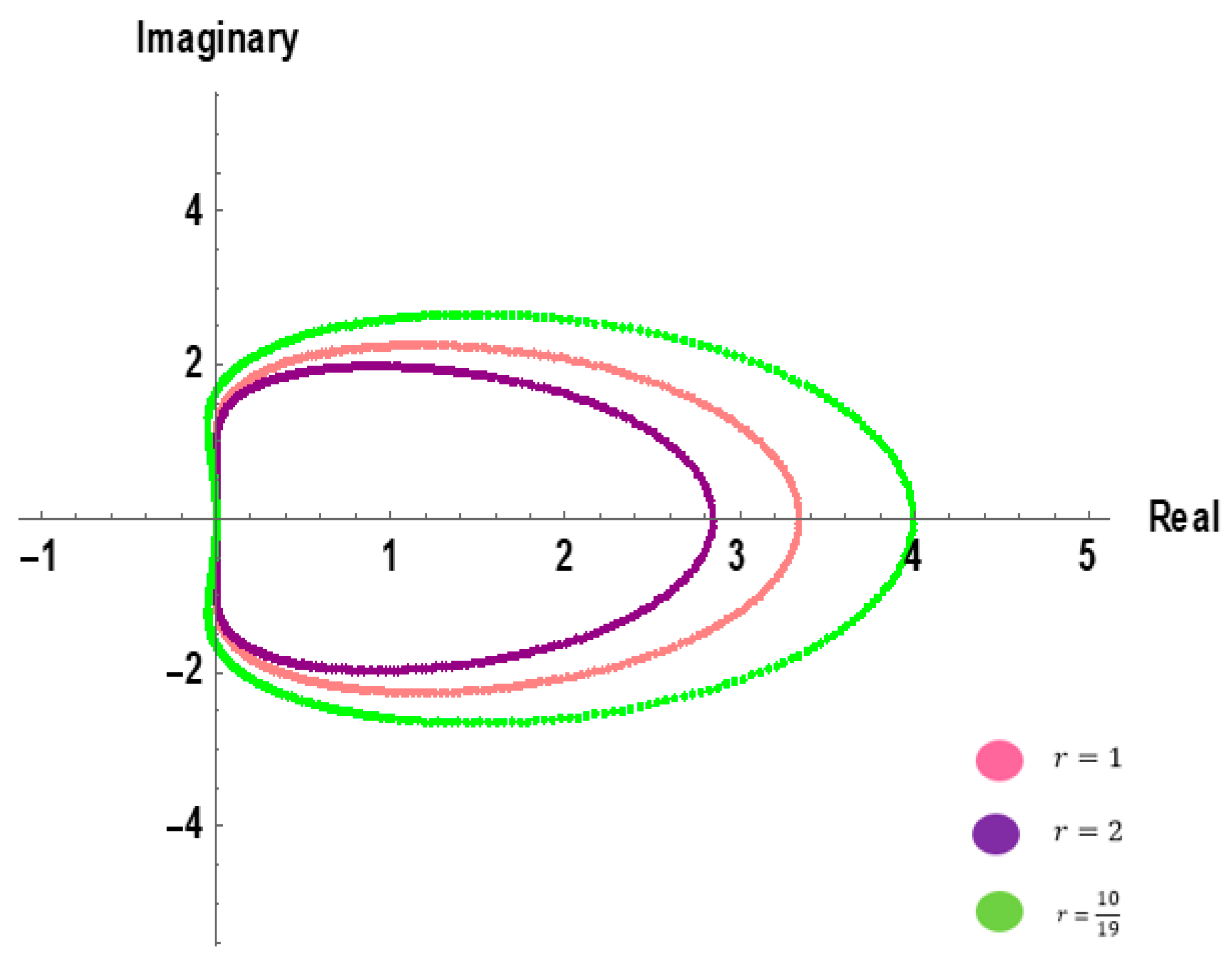
3.2. Stability Regions

Stability regions of the system are plotted in this section, using the stability polynomials given in Equations (12)–(14). The set of points defined by t = e i θ , 0     θ     2 π describes the boundary of the stability region. To determine the boundary of the stability region, the condition of roots   ( | t |     1 )   of the stability polynomial must be tested at multiple grid points. Using variable step size ratios, Figure 2 illustrates the regions of absolute stability.
The stability region corresponding to the 3–point VSBHM is presented in Figure 2. The stability region is outside of the bounded region. The method is A-stable because the majority of the region is on the left half-plane, as defined by Definition 2. Thus, it can be implied that the developed 3–point VSBHM is appropriate for stiff problems.

4. Implementation of the 3–Point VSHBM and Selection of Step Size

4.1. Implementation of the 3–Point VSBHM

Throughout this section, the Newton-type scheme to find the approximation solutions of y n + 1 , y n + 2 , and y n + 3 with one off-step point y n + 5 2 instantaneously at every step is derived. The general forms of the 3-point VSBHM as in Equation (18)
y n + 1 = σ 2 , 1 y n + 2 + σ 5 2 , 1 y n + 5 2 + σ 3 , 1 y n + 3 + α 1 , 1 h f n + 1 + ψ 1 y n + 2 = σ 1 , 2 y n + 1 + σ 5 2 , 2 y n + 5 2 + σ 3 , 2 y n + 3 + α 2 , 2 h f n + 2 + ψ 2 y n + 5 2 = σ 1 , 5 2 y n + 1 + σ 2 , 5 2 y n + 2 + σ 3 , 5 2 y n + 3 + α 5 2 , 5 2 h f n + 5 2 + ψ 5 2 y n + 3 = σ 1 , 3 y n + 1 + σ 2 , 3 y n + 2 + σ 5 2 , 3 y n + 5 2 + α 3 , 3 h f n + 3 + ψ 3
with ψ 1 , ψ 2 , ψ 5 2 , and ψ 3   are back values. Writing Equation (18) in the matrix-vector form as
( I A ) Y n + 1 , n + 2 , n + 5 2 , n + 3 = h B F + ζ n + 1 , n + 2 , n + 5 2 , n + 3
with I = 1 0 0 0 0 1 0 0 0 0 1 0 0 0 0 1   , Y n + 1 , n + 2 , n + 5 2 , n + 3 = y n + 1 y n + 2 y n + 5 / 2 y n + 3 , A = 0 σ 2 , 1 σ 5 2 , 1 σ 3 , 1 σ 1 , 2 0 σ 5 2 , 2 σ 3 , 2 σ 1 , 5 2 σ 2 , 5 2 0 σ 3 , 5 2 σ 1 , 3 σ 2 , 3 σ 5 2 , 3 0   , B = α 1 , 1 0 0 0 0 α 2 , 2 0 0 0 0 α 5 2 , 5 2 0 0 0 0 α 3 , 3   , F n + 1 , n + 2 , n + 5 2 , n + 3 = [ f n + 1 f n + 2 f n + 5 / 2 f n + 3 ] and ζ n + 1 , n + 2 , n + 5 2 , n + 3 = [ ψ 1 ψ 2 ψ 5 / 2 ψ 3 ] .
By letting Equation (19)
F ^ n + 1 , n + 2 , n + 5 2 , n + 3 = ( I A ) Y n + 1 , n + 2 , n + 5 2 , n + 3 h B F n + 1 , n + 2 , n + 5 2 , n + 3 ζ n + 1 , n + 2 , n + 5 2 , n + 3 = 0
the generalized Newton iteration formula is then defined as
Y n + 1 , n + 2 , n + 5 2 , n + 3 ( i + 1 ) = Y n + 1 , n + 2 , n + 5 2 , n + 3 ( i ) F ^ n + 1 , n + 2 , n + 5 2 , n + 3 F ^ n + 1 , n + 2 , n + 5 2 , n + 3 .
By applying Newton’s iteration of Equation (21) to the Equation (20) to approximate the solution,
Y n + 1 , n + 2 , n + 5 2 , n + 3 i + 1 Y n + 1 , n + 2 , n + 5 2 , n + 3 i = I A h B F Y Y n + 1 , n + 2 , n + 5 2 , n + 3 i 1 I A Y n + 1 , n + 2 , n + 5 2 , n + 3 i h B F Y n + 1 , n + 2 , n + 5 2 , n + 3 i ζ n + 1 , n + 2 , n + 5 2 , n + 3
( i ) and ( i + 1 ) represent the previous and current iterations. The term F Y ( Y n + 1 , n + 2 , n + 5 2 , n + 3 ( i ) ) is the Jacobian matrix of F for Y. Equation (22) is separated into three different matrices denoted as,
E 1 , 2 , 5 2 , 3 ( i + 1 ) = Y n + 1 , n + 2 , n + 5 2 , n + 3 ( i + 1 ) Y n + 1 , n + 2 , n + 5 2 , n + 3 ( i ) ,
  A ^ = ( I A ) h B F Y ( Y n + 1 , n + 2 , n + 5 2 , n + 3 ( i ) ) ,
B ^ = [ ( I A ) Y n + 1 , n + 2 , n + 5 2 , n + 3 ( i ) h B F ( Y n + 1 , n + 2 , n + 5 2 , n + 3 ( i ) ) ζ n + 1 , n + 2 , n + 5 2 , n + 3 ]
An approximate solution to Equation (1) is obtained using a two-stage Newton-type iteration. Thus, the corresponding linear system to be solved is A ^ E 1 , 2 , 5 2 , 3 ( i + 1 ) = B ^ , where E 1 , 2 , 5 2 , 3 is the increment, A ^ and B ^ are defined as
A ^ = 1 α 1 , 1 h ( f n + 1 y n + 1 ) σ 2 , 1 α 1 , 1 h ( f n + 1 y n + 2 ) σ 5 2 , 1 α 1 , 1 h ( f n + 1 y n + 5 2 ) σ 3 , 1 α 1 , 1 h ( f n + 1 y n + 3 ) σ 1 , 2 α 2 , 2 h f n + 2 y n + 1 1 α 2 , 2 h f n + 2 y n + 2 σ 5 2 , 2 α 2 , 2 h f n + 2 y n + 5 2 σ 3 , 2 α 2 , 2 h f n + 2 y n + 3 σ 1 , 5 2 α 5 2 , 5 2 h f n + 5 2 y n + 1 σ 2 , 5 2 α 5 2 , 5 2 h f n + 5 2 y n + 2 1 α 5 2 , 5 2 h f n + 5 2 y n + 5 2 σ 3 , 5 2 α 5 2 , 5 2 h f n + 5 2 y n + 3 σ 1 , 3 α 3 , 3 h f n + 3 y n + 1 σ 2 , 3 α 3 , 3 h f n + 3 y n + 2 σ 5 2 , 3 α 3 , 3 h f n + 3 y n + 5 2 1 α 3 , 3 h f n + 3 y n + 3
and
B ^ = y n + 1 ( i ) + σ 2 , 1 y n + 2 ( i ) + σ 5 2 , 1 y n + 5 2 ( i ) + σ 3 , 1 y n + 3 ( i ) + α 1 , 1 h f n + 1 ( i ) + ψ 1 σ 1 , 2 y n + 1 i y n + 2 i + σ 5 2 , 2 y n + 5 2 i + σ 3 , 2 y n + 3 i + α 2 , 2 h f n + 2 i + ψ 2 σ 1 , 5 2 y n + 1 i + σ 2 , 5 2 y n + 2 i y n + 5 2 i + σ 3 , 5 2 y n + 3 i + α 5 2 , 5 2 h f n + 5 2 i + ψ 5 2 σ 1 , 3 y n + 1 i + σ 2 , 3 y n + 2 i + σ 5 2 , 3 y n + 5 2 i y n + 3 i + α 3 , 3 h f n + 3 i + ψ 3
To ensure efficiency, a full Jacobian evaluation is only performed after a step failure, as part of the implementation of the method [17]. To reduce the computational time, a few strategies are presented below for minimizing the Jacobian evaluation.
(1)
When a successful step occurs, a new step size will be determined. This new step size be either increased ( r = 10 19 ) or remain as in the previous step size r = 1 . Each time the step size h is increased, the new matrix Equations (24) and (25) are evaluated. If the step size h remains as r = 1 , there will be no calculations of new matrices A ^ and B ^ . Hence, it will skip the Jacobian evaluation process and the previous matrices A ^ and B ^ will be used to solve Y n + 1 , n + 2 , n + 5 2 , n + 3 i + 1 . This process is called partial Jacobian evaluation.
(2)
When a failure step occurs, the next step size will be half of the previous step size r = 2 . Here the matrices A ^ and B ^ need to be updated with the new evaluations of the Jacobian matrix. This process is called full Jacobian evaluation.

4.2. Selection of Step Size
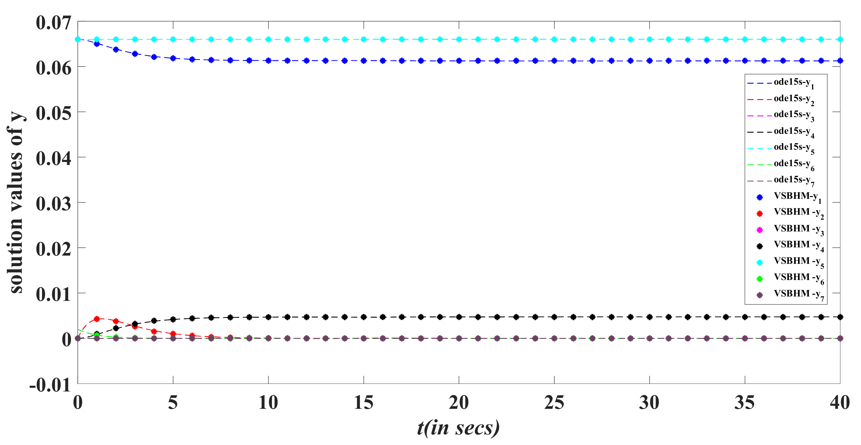
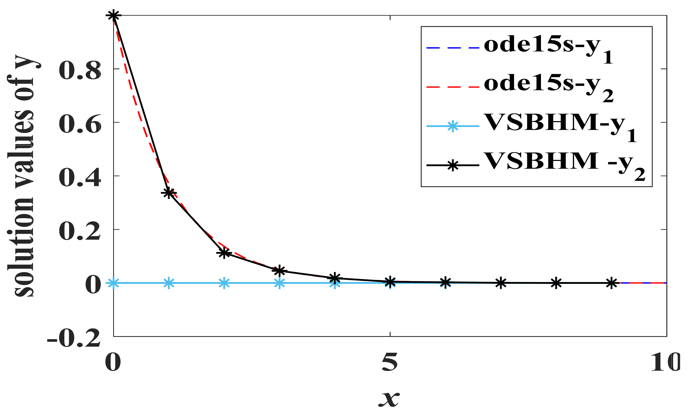
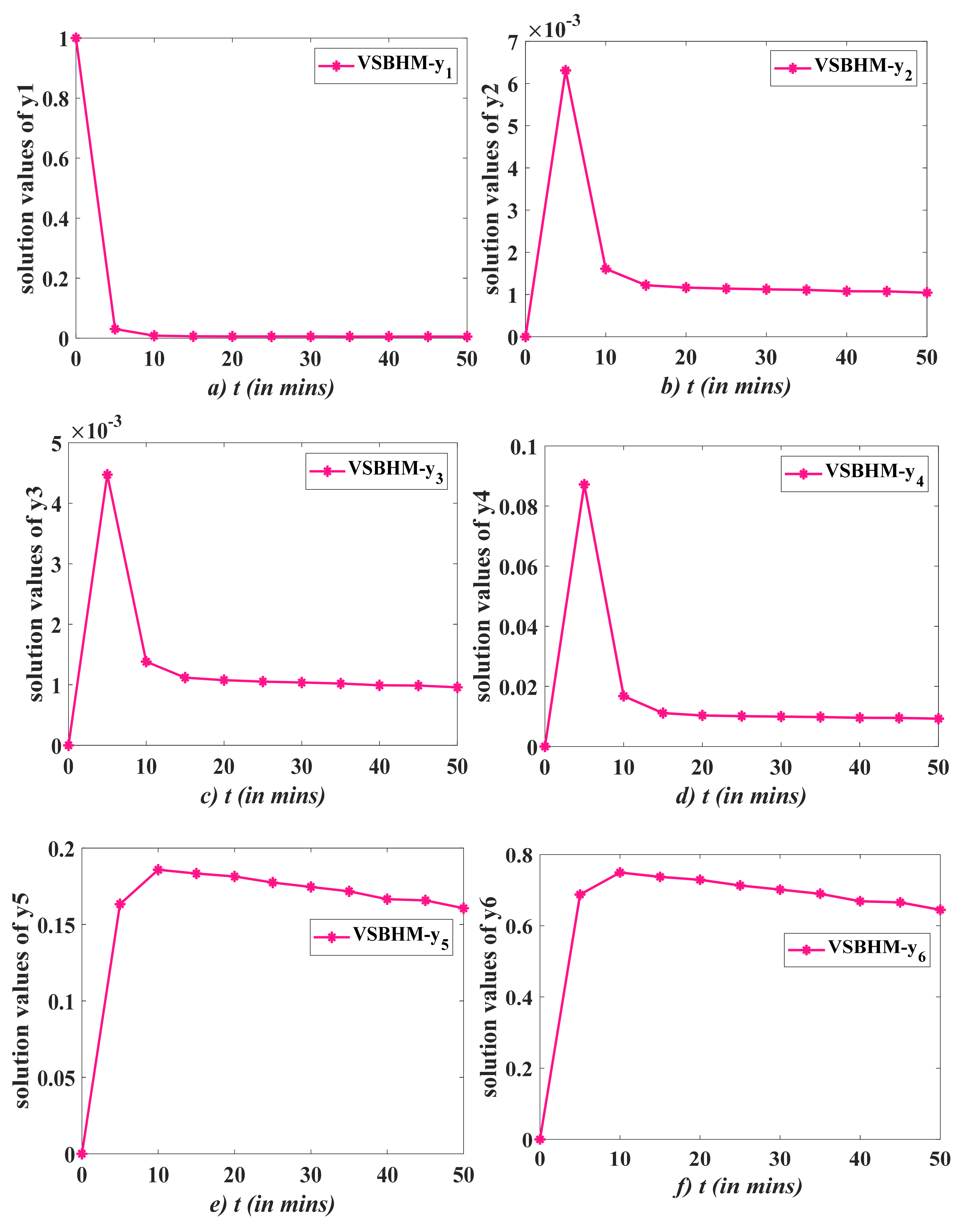
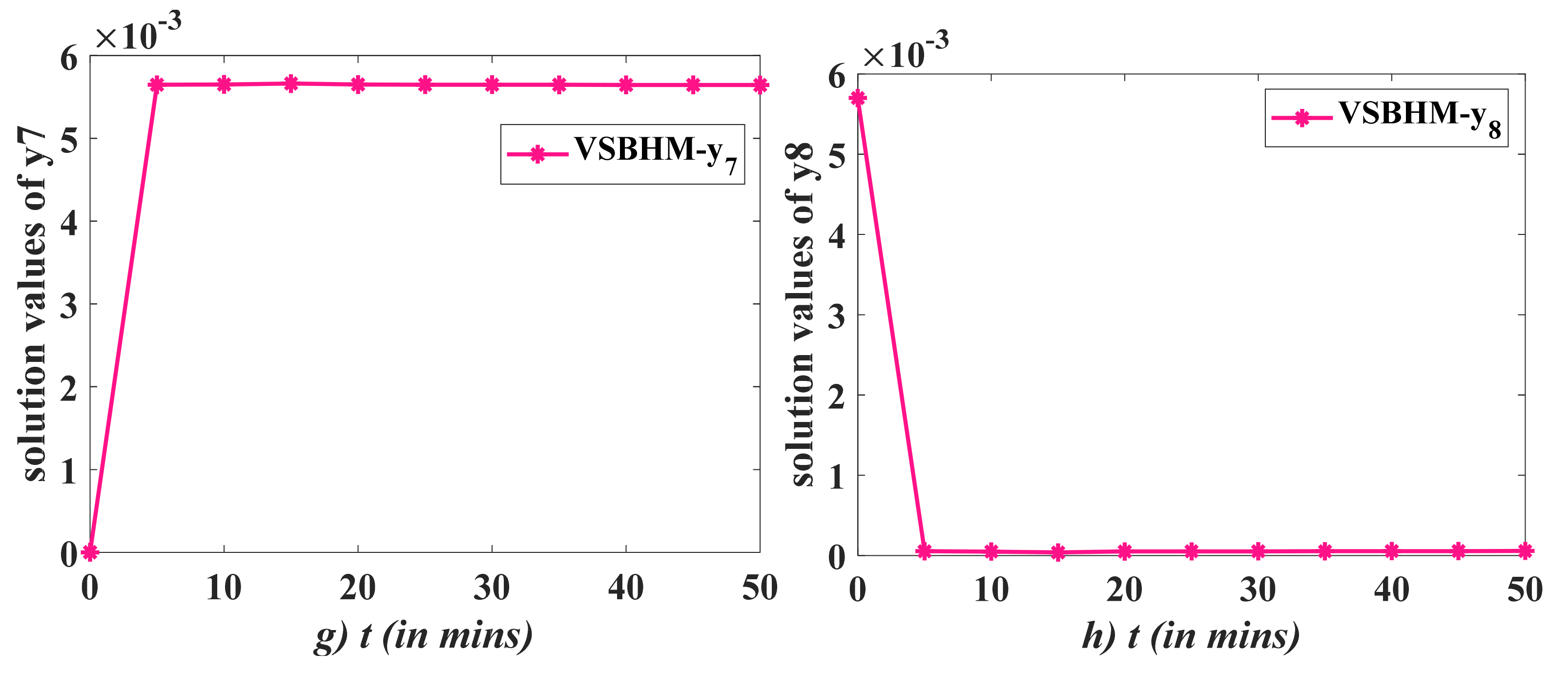
Reduction in computation time and the number of iterations can be achieved by choosing the step size properly. Throughout the process, a tolerance level (TOL) needs to be specified. If local truncation error (LTE) is less than the tolerance limit, then the values (   x n + 1 , y n + 1 ), (   x n + 2 , y n + 2 ), (   x n + 5 2 , y n + 5 2 ) and ( x n + 3 , y n + 3 ) are acceptable. The LTE can be obtained as,
LTE = y n + 3 ( p ) y n + 3 ( p 1 )
y n + 3 ( p ) is the ( p ) th order of the method and y n + 3 ( p 1 ) is the ( p 1 ) th order of the method. If the LTE > TOL then the values of y n + 1 , y n + 2 , y n + 5 2 and y n + 3 are rejected, then the step is repeated by halving the current step size ( r = 2 ) . After a successful step ( LTE < TOL ), the step size increment is given by
h n e w = c h o l d ( TOL LTE ) 1 p
and if
h n e w > 1.9 h o l d   then   h n e w = 1.9 h o l d
Safety factor c is set as 0.8 to make sure that the failure steps are being reduced, p shows the order of the method and h o l d is the step size from the previous block.

5. Test Problems

In this section, some stiff chemical kinetics problems are presented. These test problems are solved using the 3–point VSBHM and compared with the numerical results with ode15s. Graphical representations of results are presented in Section 6.
Example 1.
Belousov–Zhabotinskii reaction.
The following system of homogeneous chemical reactions can be used to illustrate the Belousov–Zhabotinskii reaction [2],
A + Y X , k 1 = 4.72 s 1 X + Y P , k 2 = 3 × 10 9 s 1 B + X 2 X + Z , k 3 = 1.5 × 10 4 s 1 2 X Q , k 4 = 4 × 10 7 s 1 Z Y , k 5 = 1 s 1
The letters A ,   ,   Z represent the species involved in the reactions, while the constants k i stands for the reaction rates. We just need to analyze the fluctuations in concentrations over time t , since the Belousov–Zhabotinskii reaction is homogeneous (all species are evenly distributed in the reaction space). The reaction rate constant characterizes each reaction step. The rate constants differ by several orders of magnitude, indicating that the associated ODE system is likely to be stiff. The initial conditions are determined by the species concentrations at t = 0 :
A = B = 0.066 ,   Y = X = P = Q = 0 ,   Z = 0.002 .
The reaction scheme is modeled by the following system of ODEs:
d A d t = y 1 ' = k 1 y 1 y 2
d Y d t = y 2 ' = k 1 y 1 y 2 k 2 y 3 y 2 + k 5 y 6 ,
d X d t = y 3 ' = k 2 y 3 y 2 + k 3 y 3 y 5 2 k 4 y 3 2 + k 1 y 1 y 2 ,
d P d t = y 4 ' = k 2 y 3 y 2 ,
d B d t = y 5 ' = k 3 y 5 y 3 ,
d Z d t = y 6 ' = k 3 y 5 y 3 k 5 y 6 ,
d Q d t = y 7 ' = k 4 y 3 2 ,
where the initial concentrations of the species are [ A 0 ] = y 1 ( 0 ) = 0.066 M ,   [ Y 0 ] = y 2 ( 0 ) = 0 M , [ X 0 ] = y 3 ( 0 ) = 0 M , [ P 0 ] = y 4 ( 0 ) = 0 M , [ B 0 ] = y 5 ( 0 ) = 0.066 M , [ Z 0 ] = y 6 ( 0 ) = 0.002 M and [ Q 0 ] = y 7 ( 0 ) = 0 M ( 1 M = 1 m o l . L 1 ) at the time interval in seconds t   [ 0 , 40 ] .
Example 2.
Stiff Chemical Problem.
Consider a non-linear system of differential equations of one of the chemical kinetic problems [37]:
y 1 ' = λ y 1 + y 2 2 , y 2 ' = y 2
where λ = 10 , 000 . The exact solution is y 1 ( x ) = e 2 x ( λ + 2 ) and y 2 ( x ) = e x .
Example 3.
HIRES.
This HIRES (High Irradiance Responses) problem is a first-order differential equation system of mild stiffness. It is a chemical process that simulates how light influences plant morphogenesis. Schäfer [38] hypothesized this chemical process involving eight reactants to explain plant tissue development and differentiation in the absence of photosynthesis at high levels of light irradiance. It was previously used as a test case for a block–oriented simulation system by Gottwald [39].
The corresponding differential equations are:
y 1 ' = k 1 y 1 + k 2 y 2 + k 3 y 3 + k 4 , y 2 ' = k 1 y 1 k 5 y 2 , y 3 ' = k 6 y 3 + k 2 y 4 + k 7 y 5 , y 4 ' = k 3 y 2 + k 8 y 3 k 9 y 4 , y 5 ' = k 10 y 5 + k 2 y 6 + k 2 y 7 , y 6 ' = k 11 y 6 y 8 + k 12 y 4 + k 8 y 5 k 2 y 6 + k 12 y 7 , y 7 ' = k 11 y 6 y 8 k 13 y 7 , y 8 ' = y 7 ' ,
Here   k 1 = 1.71 s 1 ,   k 2 = 0.43 s 1 ,   k 3 = 8.32 s 1 ,   k 4 = 0.0007 s 1 ,   k 5 = 8.75 s 1 ,   k 6 = 10.03 s 1 ,   k 7 = 0.035 s 1 ,   k 8 = 1.71 s 1 ,   k 9 = 1.12 s 1 ,   k 10 = 1.745 s 1 ,   k 11 = 280 s 1 ,   k 12 = 0.69 s 1 and k 13 = 1.81 s 1 are kinetic constants with the initial values y 1 = 1   mol · L 1 , y 2 = y 3 = y 4 = y 5 = y 6 = y 7 = 0   mol · L 1 and y 8 = 0.0057   mol · L 1 at the time interval t   [ 0 , 50 ] in minutes [40,41].

6. Results and Discussion

In this section, we present the results of numerical experiments obtained by the 3–point VSBHM as described in Section 3. This method is applied to chemical kinetics problems to confirm the competence of proposed stepsize changing strategies and to show the efficiency of the method. A comparison of the results is made with MATLAB stiff solver ode15s.
When integrating systems of ODEs, choosing initial conditions is typically not easy, specifically when the equations are stiff, and therefore the result is not easily predicted. In our opinion, the 3–point VSBHM allows for convergence in terms of approximate solutions is rather important. The shown Figure 3, Figure 4, Figure 5, Figure 6 and Figure 7 represent the approximate results of 3–point VSBHM when the error tolerance is less than 10 8 , 10 4 and 10 6 for Problems 1, 2, and 3, respectively.
From the given Figure 4, Figure 5 and Figure 7, it is clear that the convergence of the 3–point VSBHM approach provides a good approximation to the solution.
The concentrations of seven chemical reactions are displayed in Figure 3. The trend of concentration with respect to time demonstrates the decay of chemical reaction in Figure 3a,b,f for the solution values of y 1 ,   y 2 , and y 6 as time increases. This demonstrates that concentration has a constant behavior and does not change with respect to time. Figure 3b shows an initial quick transient phase, but as time increases, the reactions show stable behavior. Figure 3c depicts the concentration for y 3 , with the points fluctuating as time increases. In comparison to the previous Figure 3a,b,f, Figure 3d exhibits that y 4 has a distinct behavior. It shows that as time increases, there is a noticeable increase in the concentration of y 4 . Figure 3e depicts the y 5 concentration decreases at a steady rate as time increases. On the other hand, the graphical representation of Figure 3g demonstrates that there is a quick transient phase at first, but after a few seconds, the concentration displays constant behavior.
Figure 4 displays the comparisons of the concentrations by using the 3–point VSBHM and ode15s. The 3–point VSBHM can approximate the solution of stiff Problem 1. From Figure 4, it is shown that the 3–point VSBHM converges and approximates well the solution of the Belousov–Zhabotinskii reaction.
The results for Problem 2 is displayed in Figure 5 at t o l = 10 4 for 3–point VSBHM. Figure 5 elaborates the comparison of solution values with stiff solver ode15s and 3–point VSBHM from which a clear sketch for the proposed method is drawn as it almost approaches the solution values given by MATLAB stiff solver ode15s. Hence, it is shown that the 3–point VSBHM also converges and approximates well the solution for this stiff chemical problem.
Figure 6 portrays the attention towards the results for Problem 3. For the components y 1 , y 2 , y 3 , y 4 , y 5   y 6 , y 7 , and y 8 , we have chosen the interval [0, 50] in minutes. In Figure 6a, the plot shows the chemical solution for the species y 1 . The solution shows a quick decrease in concentration values for the first 5 min and shows a stable behavior after approximately 10 min. Figure 6b–d show the rapid change in the concentration values for the first 10 min and become stable after 10 min. Figure 6e,f show a similar pattern of increasing the concentration at the initial phase and keep decreasing in low values as the time increases. Whereas, Figure 6g shows a rapid increase in the concentration of y 7 at the beginning of 5 min and remains constant in behavior at its highest value with the increment in time. Figure 6h depicts totally inverse reactions to Figure 6g. The problem is made up of eight elements, which could be considered a significant number. The proposed approach also converges to the solution of ode15s as shown in Figure 7.
This chemical solution agrees well with the data reported by MATLAB in Figure 7. As seen in Figure 7, the stiffness of this problem is due to a large difference in the kinetic constants k i , which results in a very rapid initial transient. Initially, some very rapid transient reactions occur for some species such as y 1 ,   y 2 ,   y 3 , y 4 , y 7 and y 8 then stay almost constant. Hence from Figure 7, it can be concluded that because of the convergence of the developed 3–point VSBHM with ode15s, it can be used as an appropriate stiff solver for the numerical solutions of stiff chemical kinetics problems.

7. Conclusions

For the solution of the stiff chemical kinetics model, a 3–point VSBHM has been derived as shown in Section 3. The derived method shows an extensive region of stability which can be seen in Figure 2. Few IVPs originating from chemical kinetics comprised of large systems of stiff ODEs have been effectively implemented in the 3–point VSBHM, such as the Belousov–Zhabotinskii reaction and HIRES. Their results have been compared with MATLAB stiff solver ode15s. From the combined graphical representation of the problems, it can be concluded that the 3–point VSBHM techniques work appropriately and can be used as a stiff solver for the solutions of stiff chemical kinetics problems.

Author Contributions

Conceptualization, H.S. and N.Z.; methodology, H.S.; software, H.S. and N.Z.; validation, N.Z., H.S. and H.D.; formal analysis, H.D. and J.S.; writing—original draft preparation, H.S., N.Z. and N.J.; writing—review and editing, J.S. and N.J.; supervision, H.D., N.Z. and J.S.; project administration, N.Z. and H.D.; funding acquisition, N.Z. and H.D., A.A., M.A. and E.A.K. All authors have read and agreed to the published version of the manuscript.

Funding

This research was funded by a Fundamental Research Grant Scheme (FRGS) from the Ministry of Higher Education, Malaysia (Ref: FRGS/1/2019/STG06/UTP/03/2 and an International Collaborative Research Fund (015ME0-220) between Universiti Teknologi PETRONAS, Universitas Islam Indragiri and Universitas Islam Riau.

Institutional Review Board Statement

Not applicable.

Informed Consent Statement

Not applicable.

Data Availability Statement

Not applicable.

Conflicts of Interest

The authors declare no conflict of interest.

References

  1. AL-Jawary, M.; Raham, R. Numerical solution for chemical kinetics system by using efficient iterative method. Int. J. Adv. Sci. Tech. Res. 2016, 1, 367–375. [Google Scholar]
  2. Shulyk, V.; Klymenko, O.; Svir, I. Numerical solution of stiff ODEs describing complex homogeneous chemical processes. J. Math. Chem. 2008, 43, 252–264. [Google Scholar] [CrossRef]
  3. Singh, J.; Kumar, D.; Baleanu, D. On the analysis of chemical kinetics system pertaining to a fractional derivative with Mittag-Leffler type kernel. Chaos 2017, 27, 103113. [Google Scholar] [CrossRef] [PubMed]
  4. Sacks-Davis, R. Fixed leading coefficient implementation of SD-formulas for stiff ODEs. ACM Trans. Math. Softw. (TOMS) 1980, 6, 540–562. [Google Scholar] [CrossRef]
  5. Yatim, S.; Ibrahim, Z.; Othman, K.; Suleiman, M. A quantitative comparison of numerical method for solving stiff ordinary differential equations. Math. Probl. Eng. 2011, 2021, 193691. [Google Scholar] [CrossRef]
  6. Mahmood, A.S.; Casasús, L.; Al-Hayani, W. The decomposition method for stiff systems of ordinary differential equations. Appl. Math. Comput. 2005, 167, 964–975. [Google Scholar] [CrossRef]
  7. Ibáñez, J.; Hernández, V.; Arias, E.; Ruiz, P.A. Solving initial value problems for ordinary differential equations by two approaches: BDF and piecewise-linearized methods. Comput. Phys. Commun. 2009, 180, 712–723. [Google Scholar] [CrossRef] [Green Version]
  8. Enright, W.H.; Hull, T.; Lindberg, B. Comparing numerical methods for stiff systems of ODE:s. BIT Numer. Math. 1975, 15, 10–48. [Google Scholar] [CrossRef]
  9. Seinfeld, J.H.; Lapidus, L.; Hwang, M. Review of numerical integration techniques for stiff ordinary differential equations. Ind. Eng. Chem. Fundam. 1970, 9, 266–275. [Google Scholar] [CrossRef]
  10. Bassenne, M.; Fu, L.; Mani, A. Time-Accurate and highly-Stable Explicit operators for stiff differential equations. J. Comput. Phys. 2021, 424, 109847. [Google Scholar] [CrossRef]
  11. Wu, H.; Ma, P.C.; Ihme, M. Efficient time-stepping techniques for simulating turbulent reactive flows with stiff chemistry. Comput. Phys. Commun. 2019, 243, 81–96. [Google Scholar] [CrossRef]
  12. Ola Fatunla, S. Block methods for second order ODEs. Int. J. Comput. Math. 1991, 41, 55–63. [Google Scholar] [CrossRef]
  13. Byrne, G.D.; Hindmarsh, A.C.; Jackson, K.R.; Brown, H.G. A comparison of two ode codes: Gear and episode. Comput. Chem. Eng. 1977, 1, 125–131. [Google Scholar] [CrossRef]
  14. Sandu, A.; Potra, F.; Carmichael, G.; Damian, V. Efficient Implementation of Fully Implicit Methods for Atmospheric Chemical Kinetics. J. Comput. Phys. 1996, 129, 101–110. [Google Scholar] [CrossRef]
  15. Zawawi, I.S.B.M. Block Backward Differentiation Alpha-Formula for Solving Stiff Ordinary Differential Equations. Ph.D. Thesis, Universitiy Putra Malaysia, Serdang, Malaysia, 2017. [Google Scholar]
  16. Zainuddin, N.; Ibrahim, Z.B.; Othman, K.I.; Suleiman, M. Direct fifth order block backward differentation formulas for solving second order ordinary differential equations. Chiang Mai J. Sci. 2016, 43, 1171–1181. [Google Scholar]
  17. Ibrahim, Z.B.; Isk, K.I.; Othman, A.; Suleiman, M. Variable step block backward differentiation formula for solving first order stiff ODEs. Proc. World Congr. Eng. 2007, 2, 1–5. [Google Scholar]
  18. Abasi, N.; Suleiman, M.; Abbasi, N.; Musa, H. 2-point block BDF metho d with off-step points for solving stiff ODEs. J. Soft Comput. Appl. 2014, 2014, 1–15. [Google Scholar]
  19. Suleiman, M.B.; Musa, H.; Ismail, F.; Senu, N. A new variable step size block backward differentiation formula for solving stiff initial value problems. Int. J. Comput. Math. 2013, 90, 2391–2408. [Google Scholar] [CrossRef]
  20. Zawawi, I.S.M.; Ibrahim, Z.B.; Othman, K.I. Derivation of diagonally implicit block backward differentiation formulas for solving stiff initial value problems. Math. Probl. Eng. 2015, 2015, 767328. [Google Scholar]
  21. Majid, Z.A.; Bin Suleiman, M.; Omar, Z. 3-point implicit block method for solving ordinary differential equations. Bull. Malays. Math. Sci. Soc. Second Ser. 2006, 29, 23–31. [Google Scholar]
  22. Shampine, L.F.; Watts, H. Block implicit one-step methods. Math. Comput. 1969, 23, 731–740. [Google Scholar] [CrossRef]
  23. Nasir, N.; Ibrahim, Z.B.; Othman, K.I.; Suleiman, M. Numerical solution of first order stiff ordinary differential equations using fifth order block backward differentiation formulas. Sains Malays. 2012, 41, 489–492. [Google Scholar]
  24. Majid, Z.A.; Suleiman, M.; Ismail, F.; Othman, M. 2-point implicit block one-step method half Gauss-Seidel for solving first order ordinary differential equations. Mat. Malays. J. Ind. Appl. Math. 2003, 19, 91–100. [Google Scholar]
  25. Bakari, I.A.; Babuba, S.; Tumba, P.; Danladi, A. Two-step hybrid block backward differentiation formulae for the solution of stiff ordinary differential equations. Fudma J. Sci. 2020, 4, 668–676. [Google Scholar]
  26. Kashkari, B.S.; Syam, M.I. Optimization of one step block method with three hybrid points for solving first-order ordinary differential equations. Results Phys. 2019, 12, 592–596. [Google Scholar] [CrossRef]
  27. Kumleng, G.M.; Adee, S.; Skwame, Y. Implicit two step Adam-Moulton hybrid block method with two offstep points for solving stiff ordinary differential equations. J. Nat. Sci. Res. 2013, 3, 77–82. [Google Scholar]
  28. Sunday, J.; Odekunle, M.R.; Adesanya, A.O.; James, A.A. Extended block integrator for first-order stiff and oscillatory differential equations. Am. J. Comput. Appl. Math. 2013, 3, 283–290. [Google Scholar]
  29. Sunday, J.; Odekunle, M.R.; Adesanya, A.O. Order six block integrator for the solution of first-order ordinary differential equations. Int. J. Math. Soft Comput. 2013, 3, 87–96. [Google Scholar] [CrossRef] [Green Version]
  30. Adebayo, K.; Umar, A. Generalized rational approximation method via pade approximants for the solutions of IVPs with singular solutions and stiff differential equations. J. Math. Sci. 2013, 2, 327–368. [Google Scholar]
  31. Adesanya, A.O.; Odekunle, M.R.; James, A.A. Starting hybrid Stomer-Cowell more accurately by hybrid Adams method for the solution of first order ordinary differential equations. Euro. J. Sci. Res. 2012, 77, 580–588. [Google Scholar]
  32. Skwame, Y.; Sunday, J.; Ibijola, E.A. L-Stable Block Hybrid Simpson’s Methods for Numerical Solution of Initial Value Problems in Stiff Ordinary Differential Equations. Int. J. Pure Appl. Sci. Technol. 2012, 11, 45–54. [Google Scholar]
  33. Yakubu, D.; Madaki, A.; Kwami, A. Stable two-step Runge-Kutta collocation methods for oscillatory systems of IVPs in ODEs. Amer. J. Comput. Appl. Math. 2013, 3, 119–130. [Google Scholar]
  34. Yatim, S.; Ibrahim, Z.; Othman, K.; Ismail, F. Fifth order variable step block backward differentiation formulae for solving stiff ODEs. Int. J. Math. Comput. Sci. 2010, 4, 235–237. [Google Scholar]
  35. Ibrahim, Z.B.; Nasir, N.A.A.M. Convergence of the 2-point block backward differentiation formulas. Appl. Math. Sci. 2011, 5, 3473–3480. [Google Scholar]
  36. Dahlquist, G.G. A special stability problem for linear multistep methods. BIT Numer. Math. 1963, 3, 27–43. [Google Scholar] [CrossRef]
  37. Khalsaraei, M.M.; Shokri, A.; Molayi, M. The new class of multistep multiderivative hybrid methods for the numerical solution of chemical stiff systems of first order IVPs. J. Math. Chem. 2020, 58, 1987–2012. [Google Scholar] [CrossRef]
  38. Schäfer, E. A new approach to explain the “high irradiance responses” of photomorphogenesis on the basis of phytochrome. J. Math. Biol. 1975, 2, 41–56. [Google Scholar] [CrossRef]
  39. Gottwald, B. MISS-ein einfaches simulations-system für biologische und chemische prozesse. EDV Med. Und Biol. 1977, 3, 85–90. [Google Scholar]
  40. Amat, S.; Legaz, M.J.; Ruiz-Álvarez, J. On a Variational Method for Stiff Differential Equations Arising from Chemistry Kinetics. Mathematics 2019, 7, 459. [Google Scholar] [CrossRef] [Green Version]
  41. Aslam, M.; Farman, M.; Ahmad, H.; Gia, T.N.; Ahmad, A.; Askar, S. Fractal fractional derivative on chemistry kinetics hires problem. AIMS Math. 2022, 7, 1155–1184. [Google Scholar] [CrossRef]
Figure 1. 3–Point Variable Step Block Hybrid Method (VSBHM).
Applsci 12 04484 g001
Figure 2. Stability region of 3–Point VSBHM.
Applsci 12 04484 g002
Figure 3. Concentration of A ,   B , X , Y ,   P , Q , and Z computed using the 3 Point VSBHM for Problem 1. From left to right and top to bottom, Figure (ag) shows the numerical solution of the Belousov–Zhabotinskii reaction for t ∈ [0, 40] in seconds for the concentrations ( y 1 y 7 ) with the error tolerance 10 8 .
Applsci 12 04484 g003
Figure 4. Comparison graphs with the solution from ode15s for Problem 1 with t o l = 10 8 for 3–point VSBHM.
Applsci 12 04484 g004
Figure 5. Comparison graphs with the solution from ode15s for Problem 2.
Applsci 12 04484 g005
Figure 6. Concentration of eight species using 3–point VSBHM for Problem 3. From left to right and top to bottom, Figure (ah) shows the numerical solution of the HIRES problem for t   [ 0 , 50 ] in minutes for the concentrations ( y 1 y 8 )   with the error tolerance 10 6 .
Applsci 12 04484 g006aApplsci 12 04484 g006b
Figure 7. Comparison graphs using 3–point VSBHM and ode15s for Problem 3.
Applsci 12 04484 g007
Table 1. Variable Step Size Ratio Formulae.
Step Size RatioBlock PointsFormulae 3-Point VSBHM
r = 1 y n + 1 3 56 y n 1 3 5 y n + 3 y n + 2 64 35 y n + 5 2 + 3 8 y n + 3 3 2 h f n + 1
y n + 2 1 98 y n 1 + 3 35 y n 3 7 y n + 1 + 384 245 y n + 5 2 3 14 y n + 3 6 7 h f n + 2
y n + 5 2 75 9088 y n 1 + 147 2272 y n 1225 4544 y n + 1 + 3675 2272 y n + 2 3675 9088 y n + 3 + 105 142 h f n + 5 2
y n + 3 3 343 y n 1 16 245 y n + 12 49 y n + 1 48 49 y n + 2 + 3072 1715 y n + 5 2 + 12 49 h f n + 3
r = 2 y n + 1 1 150 y n 1 9 25 y n + 27 10 y n + 2 128 75 y n + 5 2 + 9 25 y n + 3 6 5 h f n + 1
y n + 2 1 675 y n 1 + 4 75 y n 16 45 y n + 1 + 1024 675 y n + 5 2 16 75 y n + 3 4 5 h f n + 2
y n + 5 2 5 3712 y n 1 + 81 1856 y n 225 928 y n + 1 + 6075 3712 y n + 2 405 928 y n + 3 + 45 58 h f n + 5 2
y n + 3 1 726 y n 1 5 121 y n + 25 121 y n + 1 225 242 y n + 2 + 640 363 y n + 5 2 + 30 121 h f n + 3
r = 10 19 y n + 1 7 , 428 , 297 27 , 429 , 800 y n 1 2523 2225 y n + 2523 712 y n + 2 107 , 648 51175 y n + 5 2 + 2523 5963 y n + 3 174 89 h f n + 1
y n + 2 2 , 476 , 099 59 , 212 , 925 y n 1 + 192 1325 y n 768 1537 y n + 1 + 49 , 152 30 , 475 y n + 5 2 768 3551 y n + 3 48 53 h f n + 2
y n + 5 2 7 , 428 , 297 239 , 750 , 656 y n 1 + 1587 15424 y n 66 , 125 223 , 648 y n + 1 + 198 , 375 123 , 392 y n + 2 198 , 375 516 , 704 y n + 3 + 345 482 h f n + 5 2
y n + 3 7 , 428 , 297 220 , 777 , 000 y n 1 4489 41 , 375 y n + 13 , 467 47 , 995 y n + 1 13 , 467 13 , 240 y n + 2 + 1 , 723 , 776 951 , 625 y n + 5 2 + 402 1655 h f n + 3
Table 2. Roots for Variable Step Size Ratio.
Step Size RatioRoots
r = 1 t = 0.00019497 ,   t = 0 ,   t = 0 ,     t = 1 .
r = 2 t = 0.000040309 , t = 0 , t = 0 and t = 1 .
r = 10 19 t = 0.000596546 , t = 0 , t = 0 and t = 1
Publisher’s Note: MDPI stays neutral with regard to jurisdictional claims in published maps and institutional affiliations.

