Six-Wheel Robot Design Methodology and Emergency Control to Prevent the Robot from Falling down the Stairs

Abstract

This paper proposes a design methodology for a six-wheeled rover that adapt to different stairs and maintain its stability based on the robot’s parameters, the kinematics constraints, the maximum height, and the minimum length of the step required to climb up and down. We also propose an emergency controller to prevent falls during the climb up or down using the contact angle measurement between wheel–ground by a laser scanner sensor on each side of the robot. Thus, the geometry terrain information and the wheel contact loss detection with the ground can be obtained. This loss of contact with the ground is a determining factor in an emergency case where the robot’s stability is at risk. Therefore, the controllers kick in to regain the wheel contact with the step, preventing the robot from falling. Simulations and experimental results when the robot climbs up and down stairs demonstrate the ability to react to possible falls.

1. Introduction

The demand for autonomous mobile robots is growing rapidly due to their services. In recent years, many robots have been on the market delivering packages [1,2]. They require some tasks to be solved, such as perceiving the environment [3,4], planning a trajectory [5], controlling [6], and avoiding obstacles [7,8]. The locomotion system of the robot is an important aspect to consider regarding the robot’s design, which depends on the environment and technical criteria such as its mobility and stability. A robot’s autonomous task also involves perceiving its environment to create a controller according to its pose and location. Wheeled robots have the particularity that their stability is guaranteed by maintaining the wheels’ contact with the ground. However, due to the different shapes of the surfaces, such as uneven terrain and steps, the robot’s wheels can lose contact with the ground and cause the robot to fall. Therefore, recognition of the geometry of the surface in real-time will allow the robot to act quickly towards maintaining its stability. The contact angle between the wheel and the ground is a critical parameter that determines the wheels’ position concerning the surface, which specifies if the robot’s wheel is climbing a vertical, inclined, or irregular surface.

The research carried out to determine the wheel’s point of contact is subject to using sensors that allow measuring or estimating this relationship. Force and torque sensors were installed in mobile robots to obtain the contact point; however, their installation is complex [9]. An array of pressure sensors also measure the normal stress distribution to accurately estimate the traction force, depending on the number of segments implemented in the sensor array [10]. Sensitive bumper skin also determines the contact with the surface, and it is possible to create controllers according to the deformation of the sensors, which incorporate a flexible substrate, allowing to determine the point of contact with precision. However, its effectiveness depends on the number of sensors in the wheel in contact with the surface [11]. Vision sensors such as mono-cameras are used to find the contact angle by installing a camera on each wheel; this method is verified only in a limited indoor environment [12]. Another method to estimate the contact angle derives from the robot’s internal sensors and kinematic equations; this method is easy to install but depends on the robot speed being different from zero [13], and algorithms to reduce the noise produced by the sensors [14].

The terrain information given by the contact angle between the wheel–ground and the robot velocity permit adjusts the velocity of each wheel based on the kinematics model. The Jacobian matrices of each wheel are calculated and then their inverse [13,15,16]. Another method of controlling the robot’s velocity is setting torque to each wheel according to dynamic analysis [17].

The performance of autonomous wheeled robots is also evaluated by robot designs [18,19,20], a complex task involving multiple design variables, objectives, constraints, and evaluation criteria [21,22,23].

The contributions of the paper are given as follows.

• The design methodology finds optimal values of design parameters by considering the kinematic constraints of the multiwheeled mobile robot and resulting in the climbable environmental geometric parameters such as the maximum height and the minimum length of the step.
• The contact angle is measured using laser scanner sensors, and the loss of contact between the wheel and the ground is monitored in real time, which activates the emergency controller that stabilizes the robot pose when climbing up and down stairs.
• Simulation and experiments demonstrate the robot’s performance using the design methodology, the contact angle method, and the emergency controller to climb up and down safely.

The rest of the paper is organized as follows. Section 2 describes the kinematic constraints and the optimization of the robot based on the Taguchi method. Section 3 describes the method of measuring the contact angle between the wheel–ground, the detection when the wheel loses contact, and the emergency controller. Section 4 shows the robot’s performance during climbing up and down in simulation and experiment on three different sizes of stairs: 6 × 17 cm, 7.5 × 25 cm, and 11 × 17 cm.

2. Kinematics Constraints and Robot Design Methodology

The robot model is described, and the kinematics constraints are analyzed to improve the robot design based on the Taguchi method. We defined the control parameters and the noise factors to obtain the sensitivity analysis. Then, we can find the optimal values of the design parameter. We also consider the kinematic constraints such as maximum height and minimum step that the robot can climb up or down to ensure that the parameters selected based on the Taguchi method are appropriate.

2.1. Robot Design and Kinematics Constraints

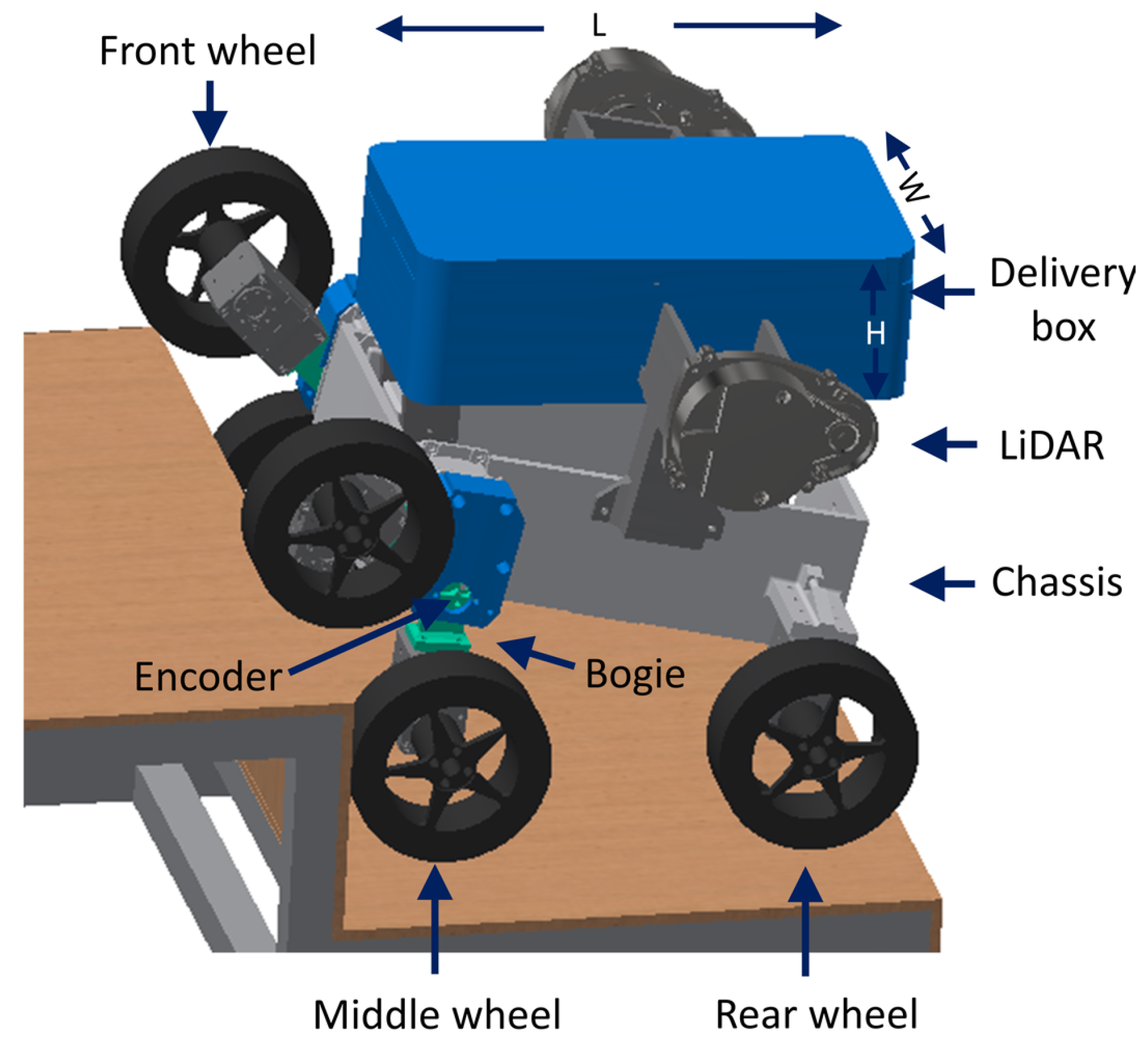
The mobile robot design comprises a chassis, a box for the delivery package, and six wheels individually controlled by each actuator, as shown in Figure 1. The front wheel $w_1$ and the middle wheel $w_2$ are attached to a passive rotation joint that denotes by bogie and Link 1, which has a triangle shape formed by $l_1$, $l_2$, and $l_4$ parameters, where $l_1$ is the distance between the center of the front wheel and the center of the bogie. $l_2$ is the distance between the center of the middle wheel and the center of the bogie. $l_4$ is the distance between the front and middle wheel. The rear wheel $w_3$ is connected to the chassis forming an imaginary link between the center of the wheel and the bogie’s center called Link 2 and $l_3$ parameter.

The center of mass of delivery package is assumed fixed above Link 1. It remains stable because the delivery box rotates and has a horizontal position with respect to the ground during the robot’s motion. $l_5$ is the distance between the bogie and the center of mass. $l_6$ is the distance between the chassis and the LiDAR.

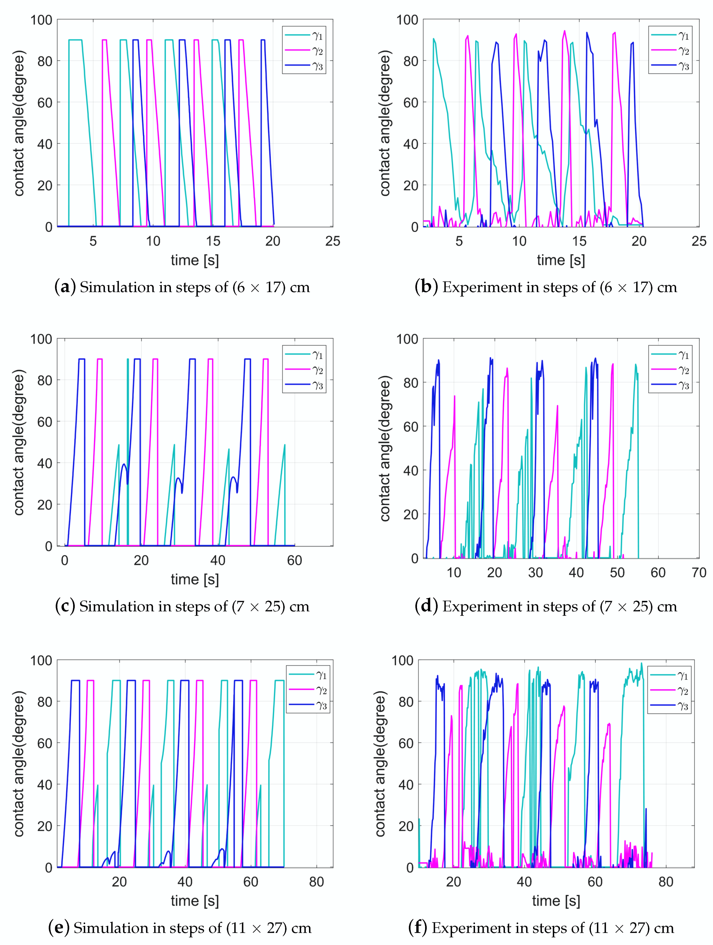
The sensors installed are encoders in each bogie to obtain the rotation measurement of the passive joint. The LiDAR sensor on each side of the robot to measure the contact angle between the wheel–ground and detect when the wheel loses contact with the ground. IMU in the chassis to obtain the rotation and the robot’s velocity. The dimensions and parameters of the robot are detailed in

Table 1. Parameters of the wheeled robot. Units in m, length (L), width (W), and height (H).

Parameters	Values(m)
chassis (L × W × H)	0.22 × 0.12 × 0.06
delivery box (L × W × H)	0.22 × 0.12 × 0.05
$r_1$	0.045
$r_2$	0.045
$r_3$	0.045
$l_1$	0.065
$l_2$	0.065
$l_3$	0.18
$l_4$	0.12
$l_5$	0.065
$l_6$	0.07

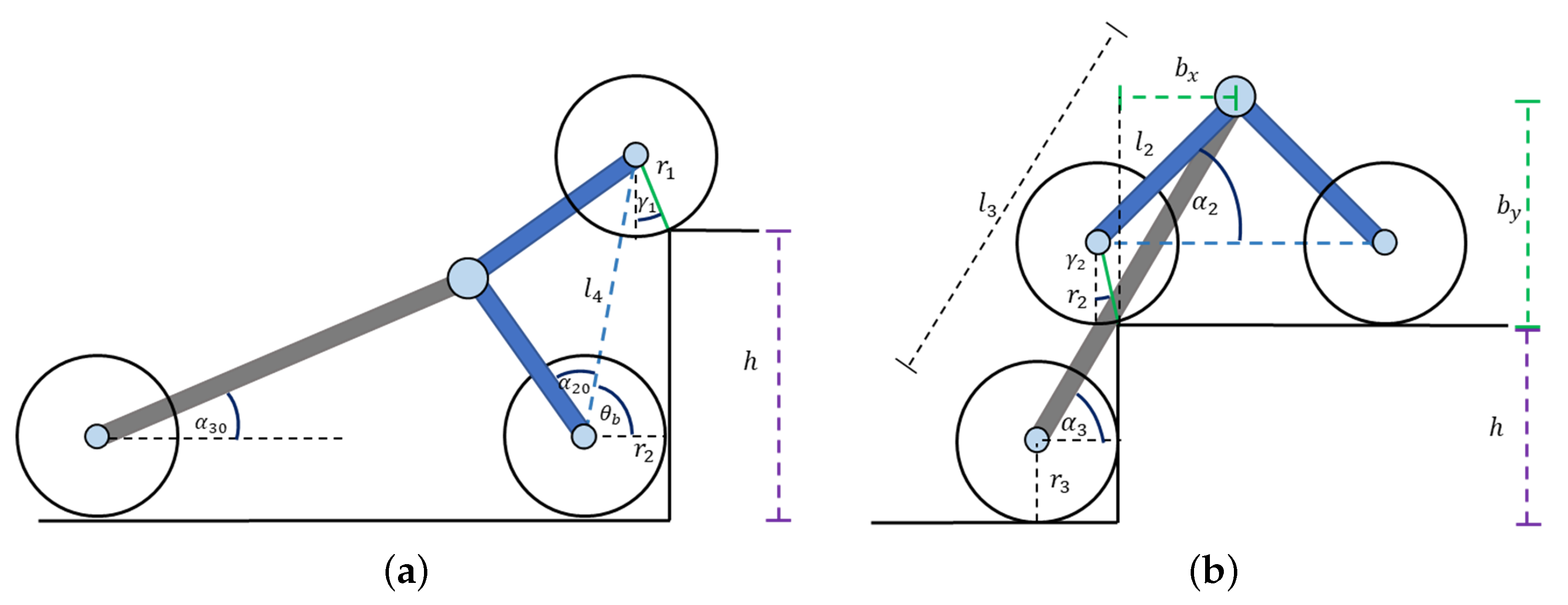
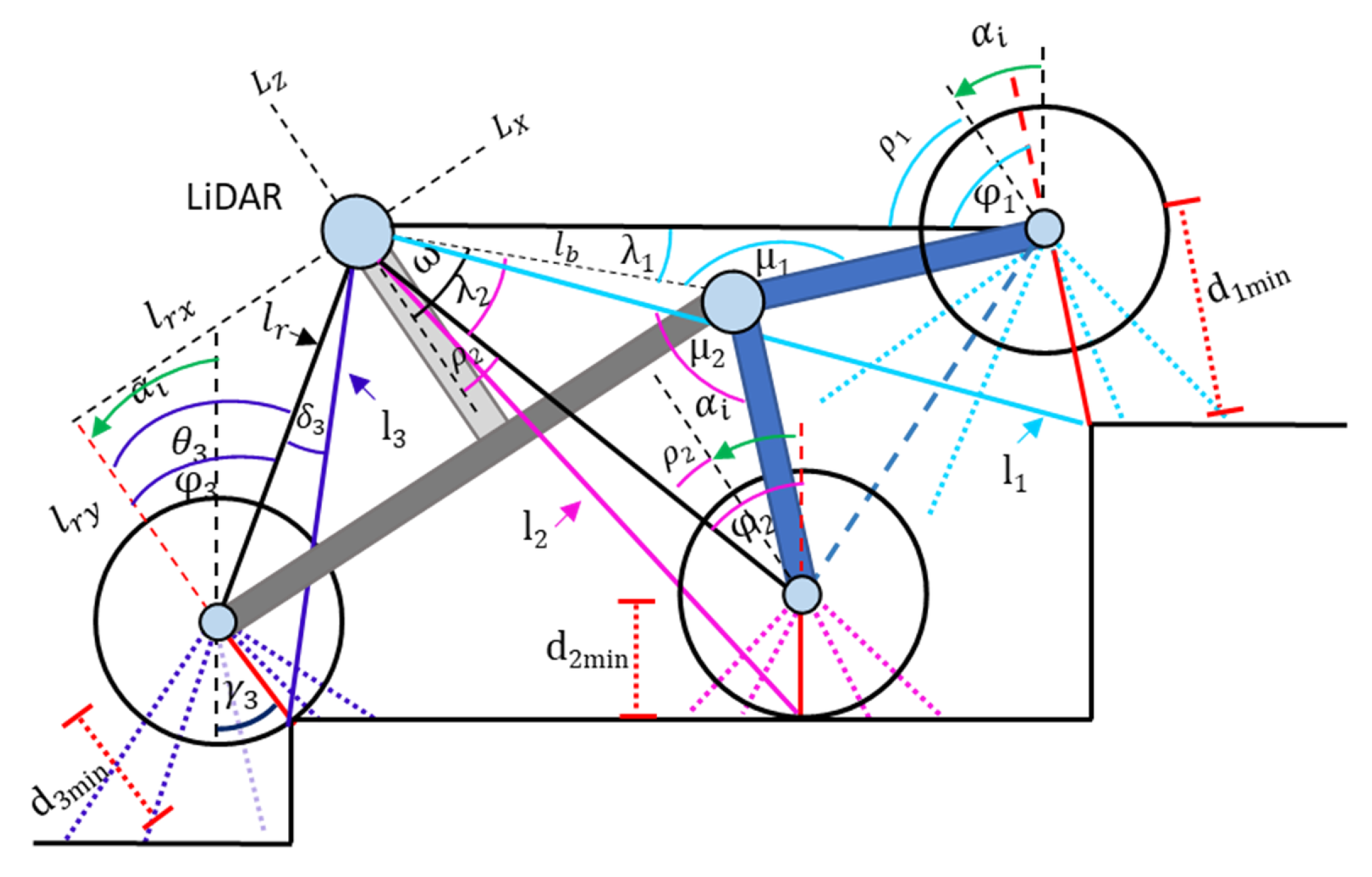
and Figure 2 shows the schematic diagram of the 2D model.

The kinematic constraints of the wheeled robot are analyzed based on the parameters and the links of the robot. Figure 2 shows the nine parameters of the robot, including the radius of the wheels, the center of mass, and the position of the LiDAR. Equation (1) details the restrictions based on the geometric relationships to prevent collision between the links and the wheels, as well as the LiDAR position according to its specifications defined as follows:

1.

Parameters $l_1$, $l_2$, and $l_4$ form Link 1. The constraints are based on keeping the link as a triangle shape to improve the robot’s stability when climbing and descending stairs.

2.

The radius of the wheels $w_1$, $w_2$, and $w_3$ must be smaller than the parameters $l_1$, $l_2$, and $l_3$, respectively, to avoid collisions between the wheels and parameters.

3.

The sum of $r_1$ and $r_2$ must be greater than $l_4$ to avoid collisions between the front and middle wheel, $w_1$ and $w_2$, respectively.

4.

The difference between $l_3$ and $r_3$ must be greater than the sum of $l_2$ and $r_2$ to avoid collisions between the middle and rear wheels, $w_2$ and $w_3$ respectively, when the robot climbs or descends stairs.

5.

The distance between the LiDAR position to the ground must be greater than 120 mm to ensure the accuracy of the contact angle results. According to the datasheet of LDS-01 from (120–499) mm, the accuracy of the distance is $\pm 15$ mm.

$$\begin{array}{cc}\hfill l_2& +l_4>l_1;l_1+l_4>l_2;l_1+l_2>l_4;\hfill \\ \hfill r_i& >l_i;\hfill \\ \hfill r_1& +r_2<l_4;\hfill \\ \hfill l_3& -r_3\ge l_2+r_2;\hfill \\ \hfill l_6& +2r_2\ge 0.12;\hfill \end{array}$$

(1)

One of the conditions for the robot to be autonomous is recognizing the obstacles in front of it and determining if they can be scaled; otherwise, the robot must take another path. It is expected that the wheels maintain contact with the ground to avoid falls. However, in reality, the wheels can lose contact; therefore, they lose their stability and fall. To ensure the robot can climb, we calculate the maximum height and the minimum length of the step that the robot can climb up and down an obstacle or step as shown in Figure 3. The maximum height can vary according to the size of the robot. Five different maximum height steps are obtained based on the constraints and parameters of the robot Equation (2), where ${\gamma }_i$ is the contact angle between each wheel and the ground, ${\alpha }_{20}$ denotes the angle between $l_2$ and $l_4$, ${\alpha }_2$ denotes the angle between $l_2$ and the horizontal global axis, ${\theta }_b$ denotes the maximum bogie rotation, ${\alpha }_{30}$ denotes the initial angle between $l_3$ and the horizontal global axis when the robot is in a flat surface, and ${\alpha }_3$ denotes the angle between $l_3$ and the horizontal that varies with the tilt of the chassis. $b_x$ denotes the horizontal distance between the center of the bogie and the contact point of the middle wheel, and $b_y$ denotes the vertical distance from the center of the bogie to the contact point of the middle wheel.

The maximum height the robot can climb up or down an obstacle is determined by Equation (3) after obtaining the maximum heights for each constraint.

• $h_1$ prevents the front and middle wheel from climbing up or down together, as shown in Figure 3a. The middel wheel maintains contact with the ground before starting to climb, and the front wheel must maintain a contact angle fewer than 65 degrees, based on experiments.
• $h_2$ is the maximum rotation of the bogie in the counterclockwise direction Figure 3a.
• $h_3$ is the maximum rotation of the bogie in a clockwise direction Figure 3b.
• Similar to $h_1$, $h_4$ restricts the middle and rear wheels from climbing up or down simultaneously Figure 3b.
• $h_5$ is the maximum height step according to the maximum inclination of the chassis to avoid falls, obtained from Figure 3b.

$$\begin{array}{cc}\hfill h_1& =\sqrt{l_4^2-(r_2-r_{1}sin{\left({\gamma }_1\right)}^2}-r_{1}cos\left({\gamma }_1\right)+r_2\hfill \\ \hfill h_2& =l_{4}sin({\alpha }_2-{\alpha }_{20})-r_{1}cos\left({\gamma }_1\right)+r_2\hfill \\ \hfill h_3& =l_{3}sin({\theta }_B+{\alpha }_{30}+{\alpha }_2-{\alpha }_{20})-b_y+r_3\hfill \\ \hfill h_4& =\sqrt{{l_3}^2-{(r_3+b_x)}^2}-b_y+r_3;\hfill \\ \hfill h_5& =l_{3}sin{\alpha }_3-b_y+r_3;\hfill \end{array}$$

(2)

$$min\left(h_i\right)=h_{max}$$

(3)

The minimum length of the step required to climb up or down depends on the step height h, which must be less than $h_{max}$ Equation (3). The first case is when h is equal to $h_{max}$, the minimum length of the step when the robot climbs up is the length of $l_4$ plus $r_1$, $r_2$, and the horizontal distance between the middle and rear-wheel contact point. However, when the robot climbs down with $h_{max}$, the minimum step length required is the total length of the robot. The second case occurs when the front and middle wheel maintain contact with the tread or the middle and rear wheel maintain contact with the tread. Then we include a parameter d, which is the distance between the middle wheel and the step. If the parameter d is greater than zero, there is a space between the middle wheel and the step. Furthermore h is less than $h_{max}$ and we can obtained $t_1$ and $t_2$. $t_1$ denotes the horizontal distance between the front and middle wheel in contact with the tread, including both wheel’s radius, and $t2$ denotes the horizontal distance between the middle and rear wheel in contact with the tread, including both wheel’s radius. The middle wheel can climb up or down with fewer than 65 degrees of contact angle. This value is obtained based on experimentation. Then, the largest distance between $t_1$ and $t_2$ is the minimum distance required if two wheels simultaneously touch the tread. Finally, the third case is when the robot can climb up and down, and the three wheels maintain contact with the ground in three different steps. The minimum tread required is subject to the maximum slant of the chassis during climbing up or down.

2.2. Robot Design Methodology

Designing a robot based on experience and trial and error does not ensure that the chosen parameters and the combination of these offer the best results for the robot’s performance. The robot design implies multiple variables, objectives, restrictions, and evaluation criteria.

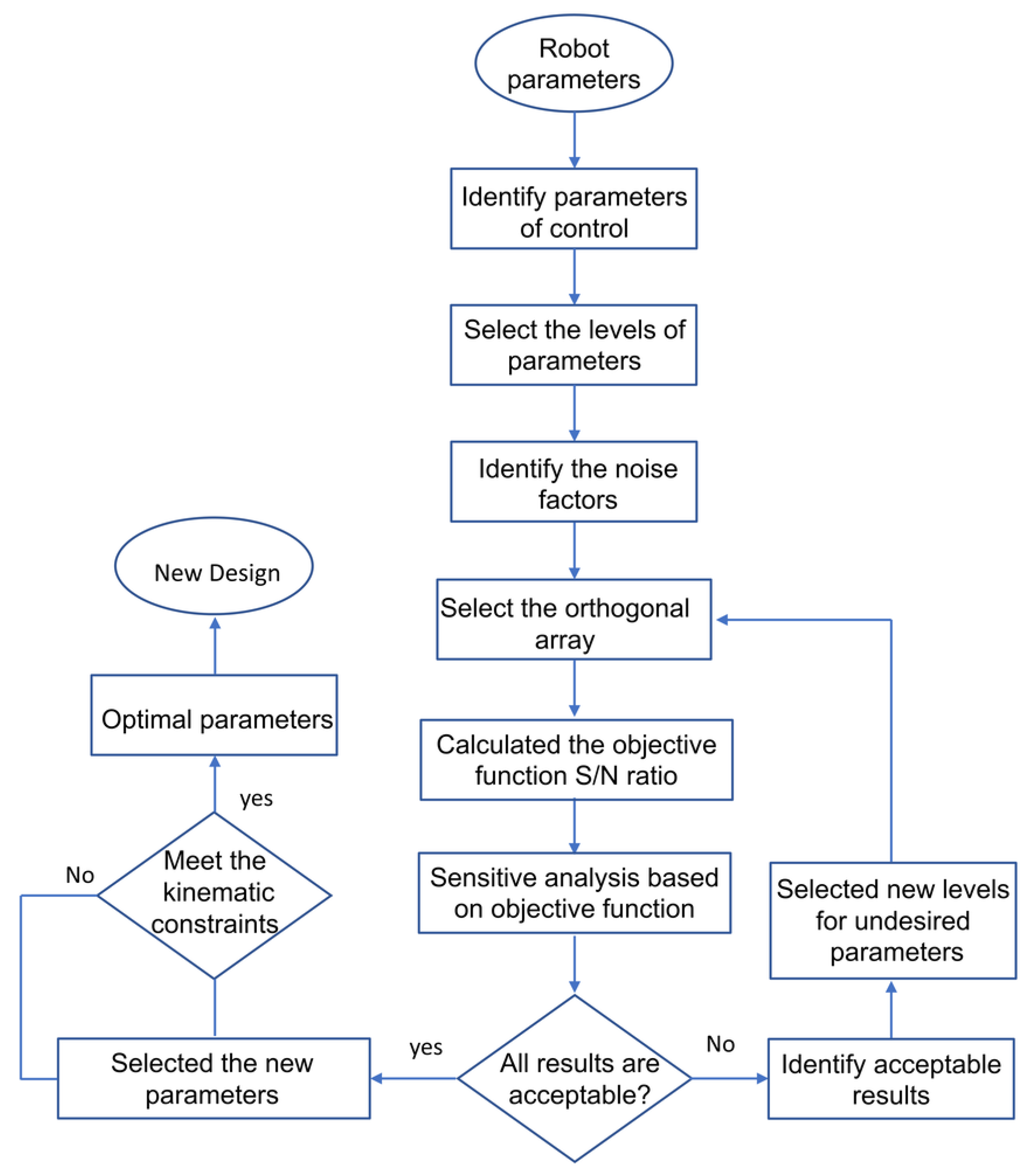
The robot design methodology proposed in this paper is described in Figure 4. The flowchart shows how the designer obtained the optimal parameters for the wheeled robots. We identify the parameters of control, which are the length of the links and the wheel radius. These parameters are changeable and evaluated to improve the robustness of the robot. We selected three levels of each parameter based on the kinematic constraints. The noise factor is a variable that cannot be controlled. For example, we do not know the height and the minimum step that the robot can find on its way. Then, we chose three different stair sizes as noise factors to ensure the robot could climb up and down different sizes of steps. We selected the orthogonal array according to the number of control factors and the levels. Then, we calculated the signal–noise ratio according to the objective function and obtained the sensitivity analysis. If the results show higher slopes between the levels of each parameter, it means we can select new levels and evaluate them again. We can select the best values based on the objective function if the slopes are minimums. Finally, if the new design parameters meet the kinematic constraints, they can be considered optimal design parameters.

The Korea Electronics Technology Institute (KETI) designed the six-wheeled mobile robot [24,25], and we adapted it to the robot shown in Figure 1. The optimization is carried out under the Taguchi method [26,27,28]. We find the optimal combination parameters and improve its performance based on minimizing the trajectory of the center of mass and the slope of 3 different stairs. The results obtained show the robustness of the robot through the analysis of the signal-to-noise (S/N) ratio.

For the simplicity of the robot design, nine parameters are chosen, as shown in Table 1. For the methodology design, the six most relevant parameters shown in

Table 2. Wheeled robot parameters chosen as control factors at three different levels.

	Control Factors [mm]
Level	$l_1$	$l_2$	$l_4$	$r_1$	$r_2$	$r_3$
1	70	70	125	45	45	45
2	65	65	120	35	50	50
3	75	75	115	30	35	40

, these parameters represent the links and joints of the robot. Although the dynamic parameters affect the robot’s behavior, we can safely create a proper robot control to climb up and down stairs with the kinematic analysis. The dimensions of the chassis and the delivery box remain fixed as $l_3$, $l_5$, and $l_6$, since these values keep the original design. Therefore, the control factors are $r_1$, $r_2$, $r_3$, $l_1$, $l_2$, and $l_4$.

In addition, three levels are determined for each parameter to optimize the design. These values were based on the kinematic analysis. Thus, it reduces the time of experimentation and analysis to find the optimal values. The levels are shown in Table 2. Since there are six parameters and three levels, we selected the orthogonal array $L_{27}\left(3^6\right)$.

The evaluation of the three levels is given by the signal-to-noise ratio (S/N), where “signal” represents the desired value and “noise” represents the undesirable value. Lower signal noise means the design is robust.

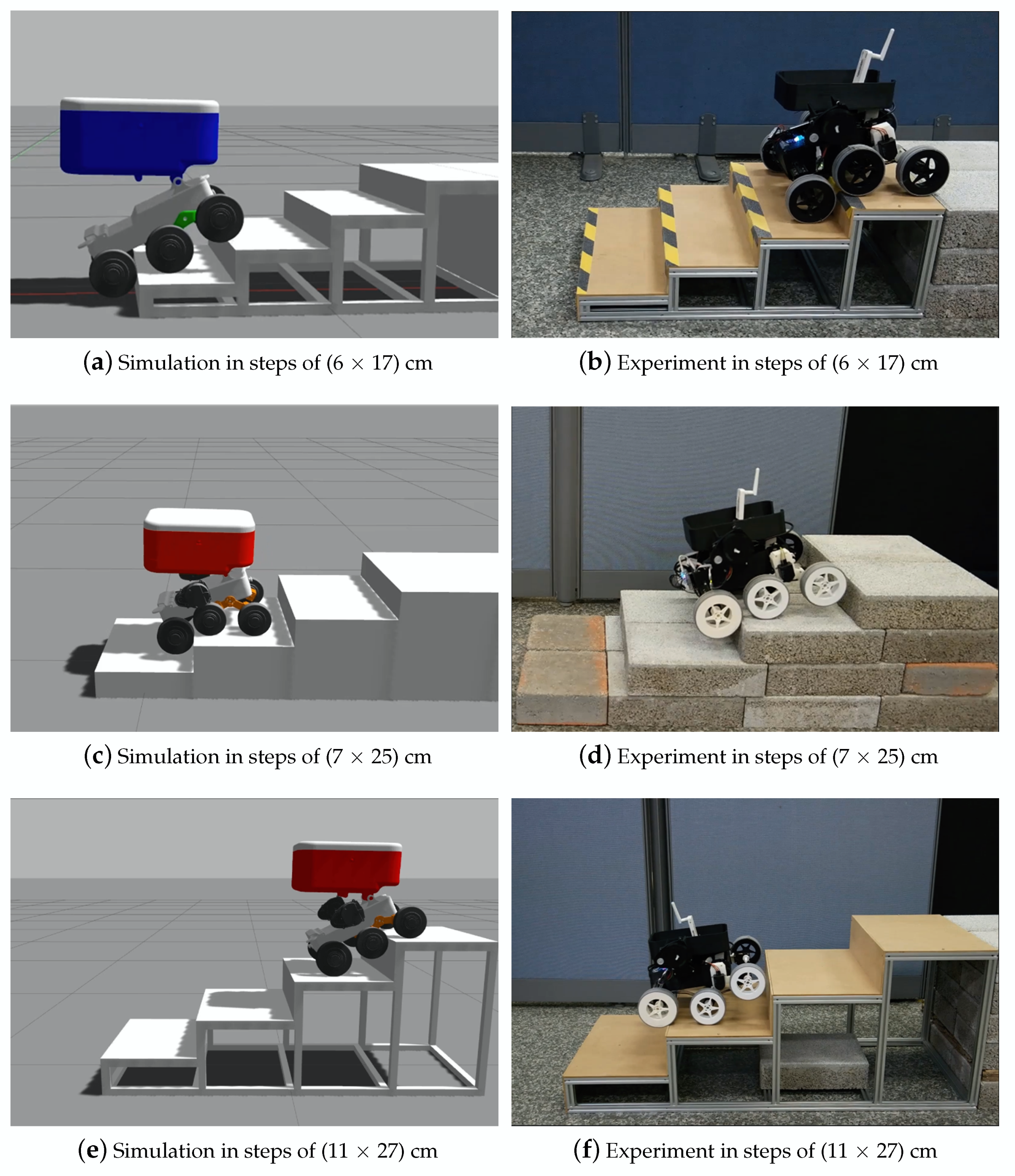
The optimal design parameters are given by sensitive analysis based on the signal–noise ratio Equation (4). The goal is to reduce the trajectory of the center of mass as low as possible to the slope of the stair, maintaining the wheels’ contact with the ground. Therefore, the robot is more robust and adapts to different sizes of stairs. n is the number of experiments conducted at level i, in our case, three sizes of stairs: $(6\times 17)$ cm, $(7.5\times 25)$ cm, and $(11\times 27)$ cm. $y_i$ is the area between the slope of the stair and the center of mass trajectory. To find the optimal values, we expect to choose the most positive values of the S/N ratio in each parameter and check the kinematic constraints to ensure that the robot can satisfy the requirements to climb up and down stairs.

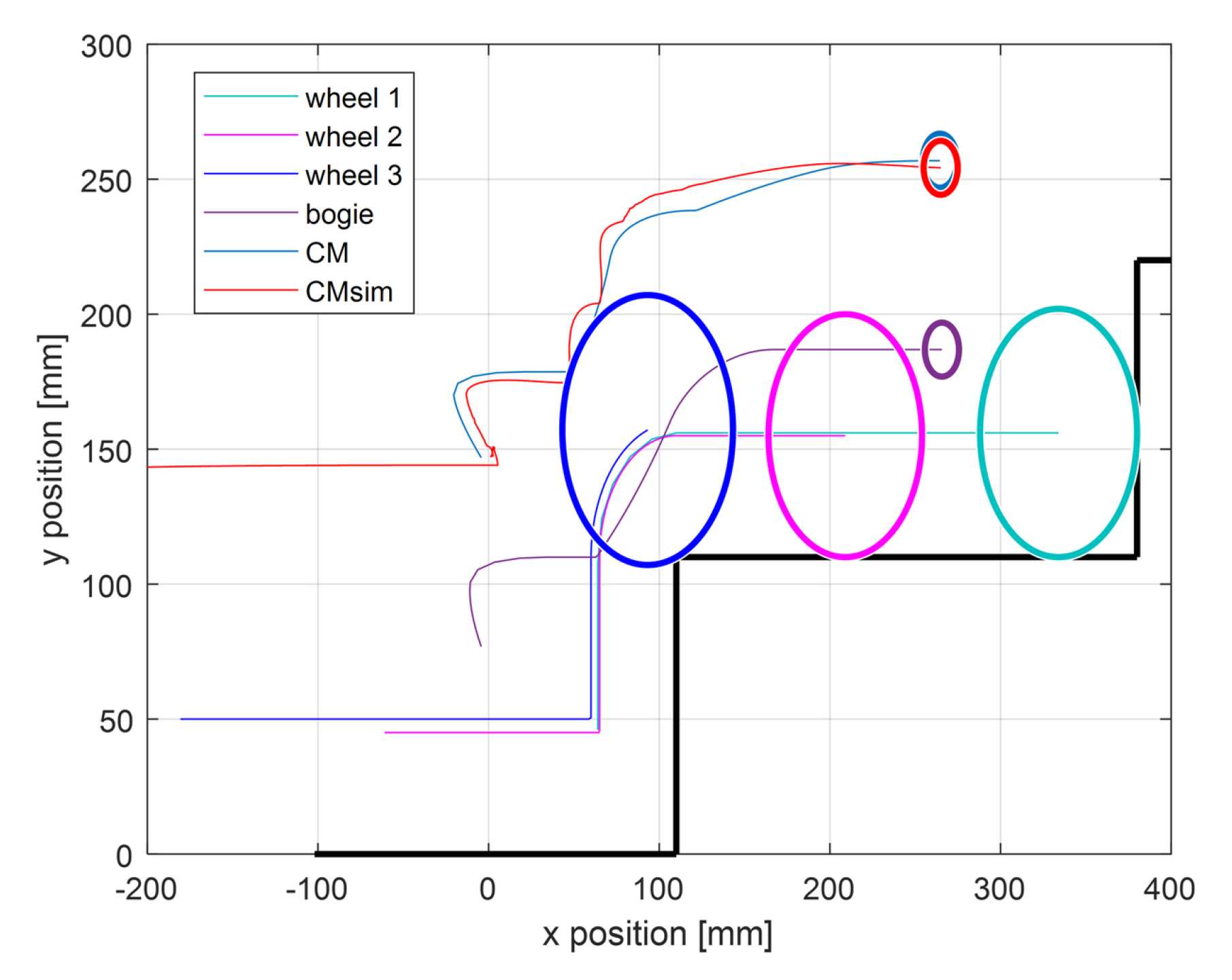
The center of mass considered in the paper is the CM of the delivery package, including the load. Figure 5 shows the trajectory of the bogie, wheels, and center of the mass from the robot design while climbing up a step of $(11\times 27)$ cm, obtained by the kinematic relation between wheels and links. Furthermore, $C{M}_{sim}$ denotes the trajectory of the center of mass obtained in the Gazebo simulator using ROS. Therefore, we can validate that the center of mass can be assumed to be fixed above Link 1 as long as the motor maintains the delivery package in a horizontal position during the robot’s motion.

From the orthogonal array $L_{27}\left(3^6\right)$ and the three levels of each parameter, we obtain $y_i$. Therefore, we calculate S/N Equation (4).

Table 3. First iteration $L_{27}\left(3^6\right)$ array from Taguchi method.

Control Factors [mm]							Objective Function [mm]			[dB]
Test	$l_1$	$l_2$	$l_4$	$r_1$	$r_2$	$r_3$	$y_1$	$y_2$	$y_3$	S/N
1	70	70	125	45	45	45	1474	5603	8887	−75.74
2	70	70	125	45	50	50	1603	5593	9461	−76.14
3	70	70	125	45	35	40	1285	4968	7774	−74.61
4	70	65	120	35	45	45	1802	6214	9707	−76.57
5	70	65	120	35	50	50	2007	6558	10,313	−77.09
6	70	65	120	35	35	40	1480	5539	8923	−75.74
7	70	75	115	30	45	45	2738	7519	11,872	−78.35
8	70	75	115	30	50	50	2939	7850	12,329	−78.70
9	70	75	115	30	35	40	2264	6850	10651	−77.42
10	65	70	120	30	45	50	2327	7028	11,030	−77.70
11	65	70	120	30	50	40	2536	7302	11,500	−78.06
12	65	70	120	30	35	45	2123	6372	10,238	−76.99
13	65	65	115	45	45	50	1642	5971	9315	−76.20
14	65	65	115	45	50	40	1819	5910	9813	−76.52
15	65	65	115	45	35	45	1360	5315	8715	−75.48
16	65	75	125	35	45	50	2130	6392	10,642	−77.23
17	65	75	125	35	50	40	2331	6643	10,603	−77.32
18	65	75	125	35	35	45	1753	6117	9504	−76.40
19	75	70	115	35	45	40	1901	6428	10,487	−77.13
20	75	70	115	35	50	45	2156	6833	10,855	−92.03
21	75	70	115	35	35	50	1664	5948	9525	−76.33
22	75	65	125	30	45	40	1754	6136	9678	−76.51
23	75	65	125	30	50	45	1954	6485	10,275	−77.03
24	75	65	125	30	35	50	1633	5774	8971	−75.89
25	75	75	120	45	45	40	1434	5681	9030	−75.87
26	75	75	120	45	50	45	1624	6070	7630	−75.13
27	75	75	120	45	35	50	1366	4979	8246	−74.99

shows the result of the Taguchi method. The result of the initial design is $-75.74$ [dB]. This result is acceptable because prior to the construction of the robot and the stairs, we analyzed the kinematic constraints to know the maximum height the robot could climb. However, in real tests, the wheels lost contact with the ground, and inevitably the robot fell. Then, we decided to implement an emergency controller to avoid falls, as detailed in the next section, and optimize the robot design in the current section.

$$S/N=-10{log}_{10}\left\{\begin{array}{c}\sum _{i=1}^n\frac{y_i^2}{n}\end{array}\right\}$$

(4)

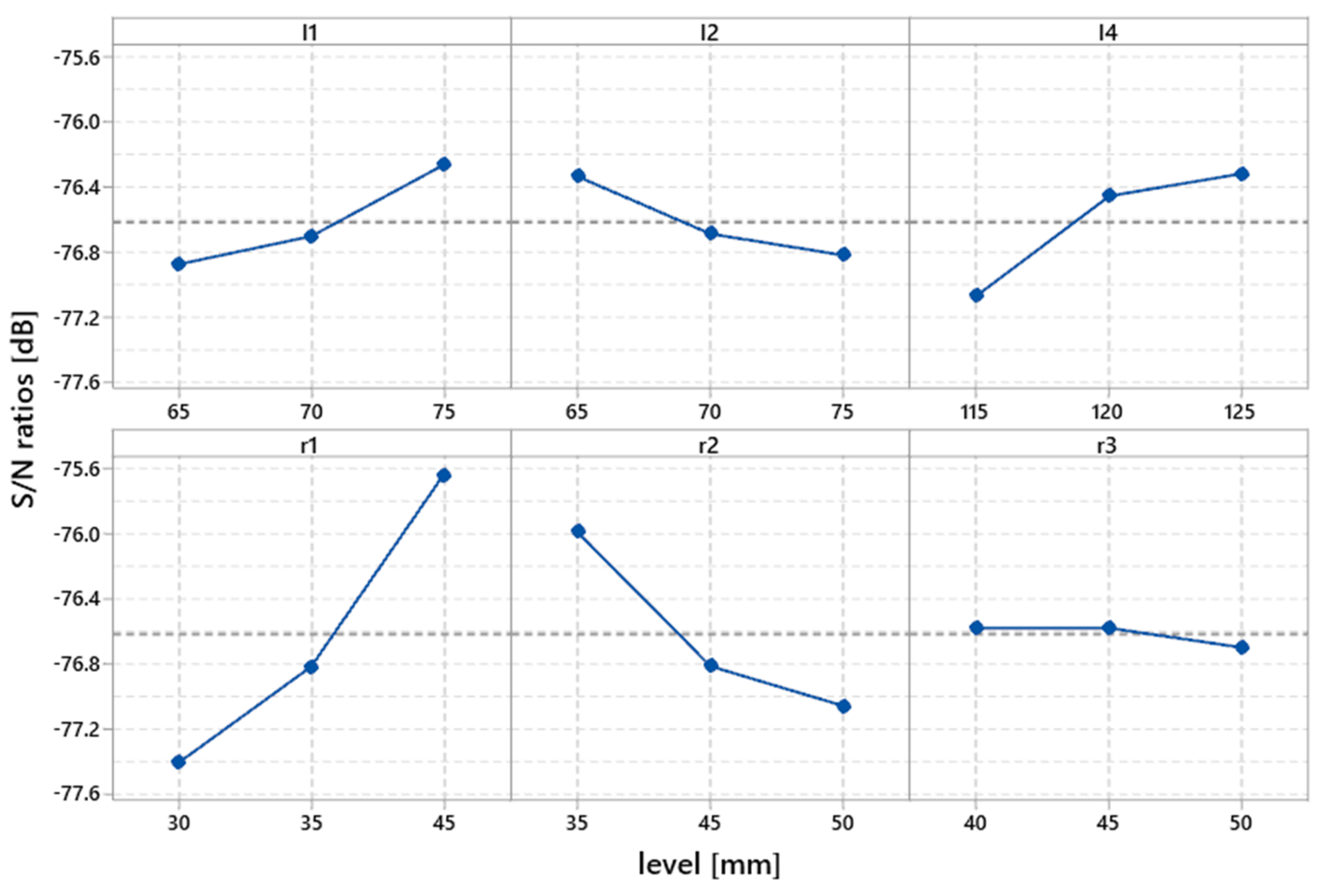
The sensitivity analysis of the Taguchi method is shown in Figure 6. The six control factors are evaluated based on the objective function. Higher values in the S/N ratio mean optimal values of the design parameters. However, suppose the slope between the levels in each parameter is high. In that case, it means having large sensitivity. Then, it is recommended to prepare a second iteration with new levels in the parameters with high sensitivity in conjunction with the optimal values in the parameters with low sensitivity effects. The parameters $l_1$, $l_2$, $l_4$, and $r_3$ have low sensitivity, and $r_1$ and $r_2$ have high sensitivity. From the first iteration results, we selected $l_1=75$, $l_2=65$, $l_4=120$, and $r_3=50$. For $l_4$, even though 125 shows a higher value in (dB), we selected 120 based on kinematic constraints to reduce the length of the robot. For $r_3$, the three values in (dB) are practically the same. Therefore, we decided to choose 50 because, during the descent of the 11 cm-high step, the rear wheel takes time to touch the ground, and the robot loses stability.

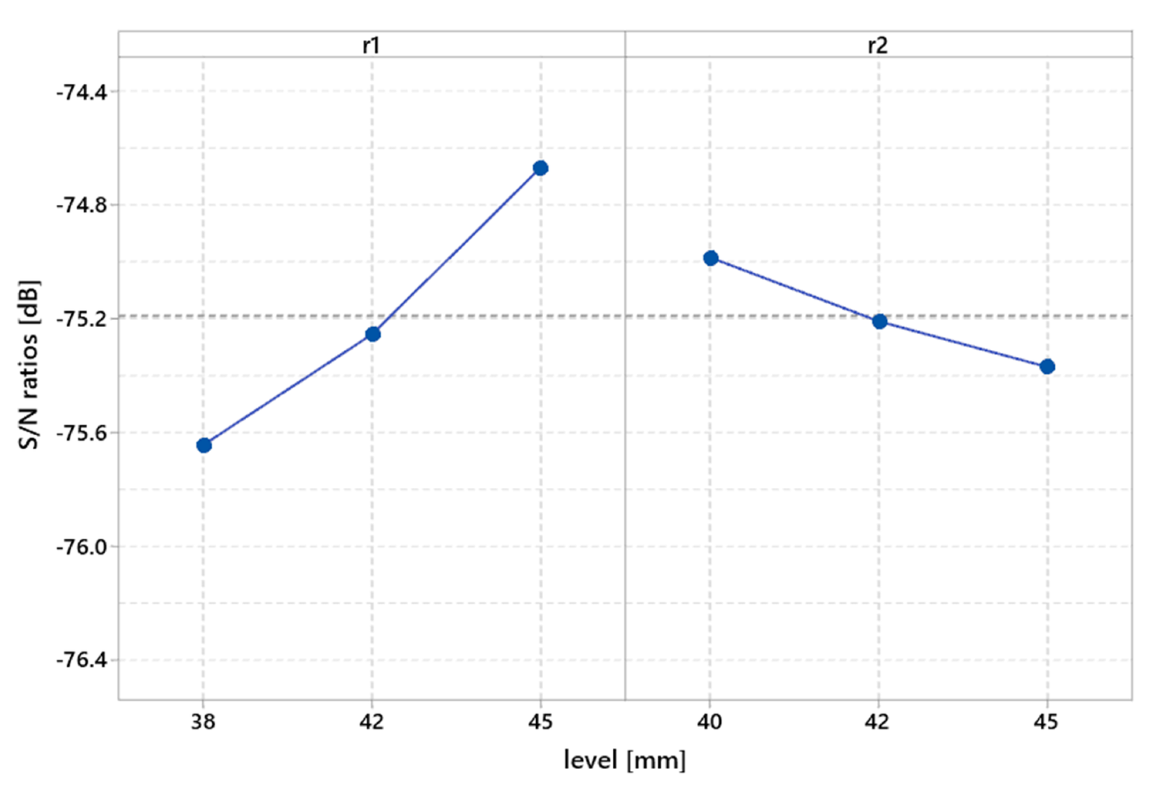
The second iteration focuses on $r_1$ and $r_2$. The optimal values obtained from the first iteration, and the three new levels for $r_1$ and $r_2$ are shown in

Table 4. Optimal values from the first iteration and three new levels for the second set of the experiment.

	Control Factors [mm]
Level	$l_1$	$l_2$	$l_4$	$r_1$	$r_2$	$r_3$
1	75	65	120	38	40	50
2				42	42
3				45	45

. The new orthogonal array is given by $L_9\left(3^2\right)$. We calculate $y_i$ and the objective function S/N ratio, as show in

Table 5. Second iteration $L_9\left(3^2\right)$ array from the Taguchi method.

	Control Factors [mm]		Objective Function [mm]			[dB]
Test	$r_1$	$r_2$	$y_1$	$y_2$	$y_3$	S/N
1	38	40	1352	5305	8730	−75.4894
2	38	42	1396	5431	8955	−75.7069
3	38	45	1468	5621	8871	−75.7382
4	42	40	1371	5192	8177	−75.0379
5	42	42	1407	5321	8395	−75.2626
6	42	45	1468	5231	8723	−75.4658
7	45	40	1227	4828	7642	−74.4308
8	45	42	1252	4952	7855	−74.6633
9	45	45	1296	5107	8074	−74.9113

.

The sensitive analysis from the second iteration is shown in Figure 7. To determine the optimal values for $r_1$ and $r_2$, we compare the S/N ratios from $-77.6$ to $-75.6$ (dB) in the first iteration, which reduces from $-75.6$ to $-74.6$ (dB) in the second iteration, these values denote better results than the previous ones. Then, we selected the optimal values in conjunction with the kinematic constraints. It is worth noting that the three levels in each parameter satisfy the kinematic constraints. Therefore, the optimal values are $r_1=45$ and $r_2=45$, even in the graph showing that $r_2=40$ has a better S/N ratio; We selected 45 because when the robot is climbing up or down the high $(11\times 27)$ cm step, the chassis rubbed against the stair.

Table 6. Initial and optimal design results of the wheeled robot after the second iteration.

Control Factors [mm]							Objective Function [mm]			[dB]
Test	$l_1$	$l_2$	$l_4$	$r_1$	$r_2$	$r_3$	$y_1$	$y_2$	$y_3$	S/N
Initial	70	70	125	45	45	45	1474	5603	8887	−75.74
Optimal	75	65	120	45	45	50	1296	5107	8074	−74.91

shows the comparison of the initial design and the optimized design, as well as the gain in (dB) being $0.84$.

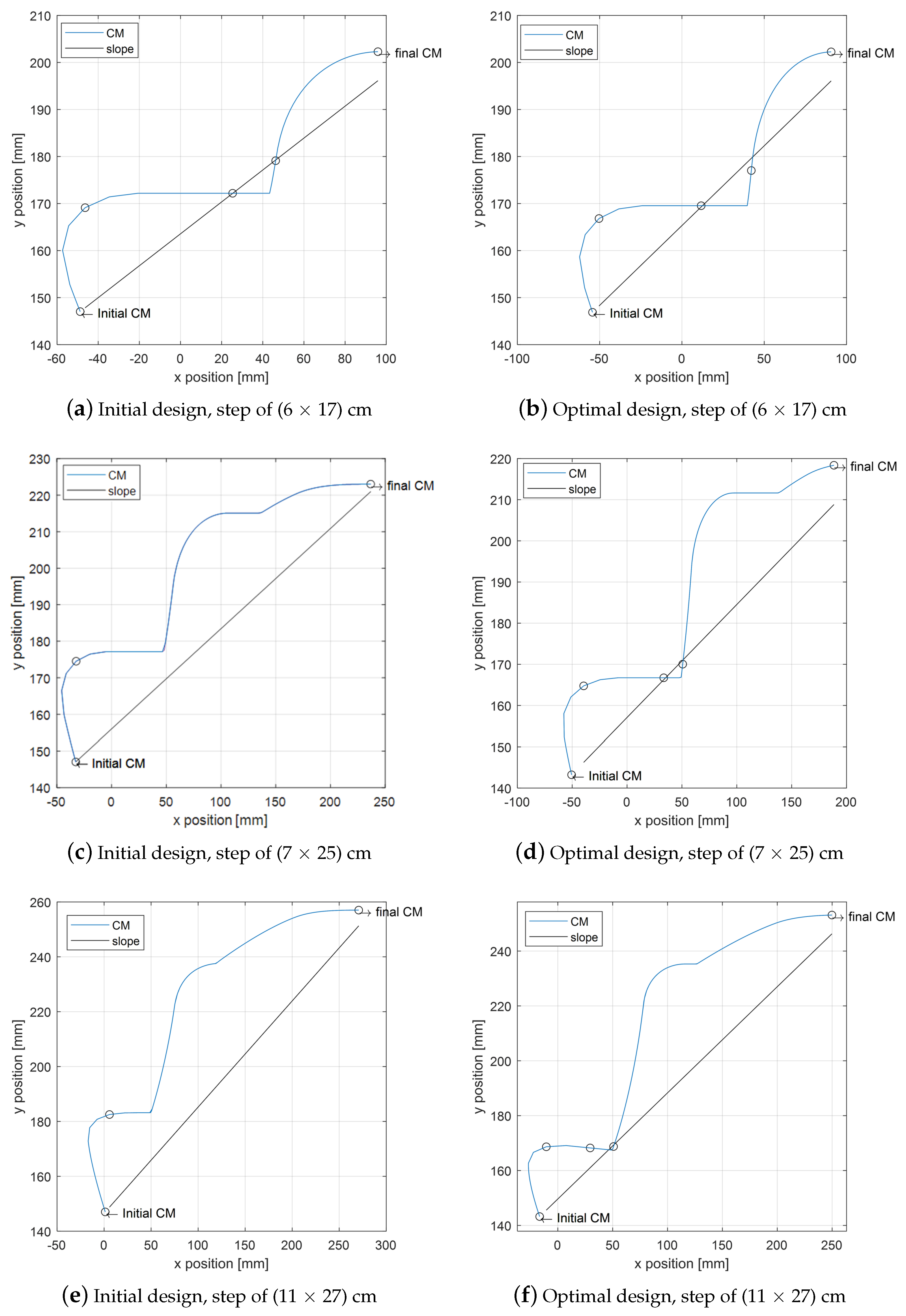
Figure 8 shows the area between the path of the center of mass and the slope of each stair. The results show satisfactorily that the area decreased with the optimal design. Figure 8a,b shows the robot climbing up one step of (6 × 17) cm, initial and optimal design, respectively; the area reduces from 1474 mm to 1227 mm. Figure 8c,d shows the robot climbing up one step of (7.5 × 25) cm, initial and optimal design, respectively; the area reduces from 5603 mm to 4828 mm. Figure 8e,f shows the robot climbing up one step of (11 × 27) cm, initial and optimal design, respectively; the area reduces from 8887 mm to 7624 mm.

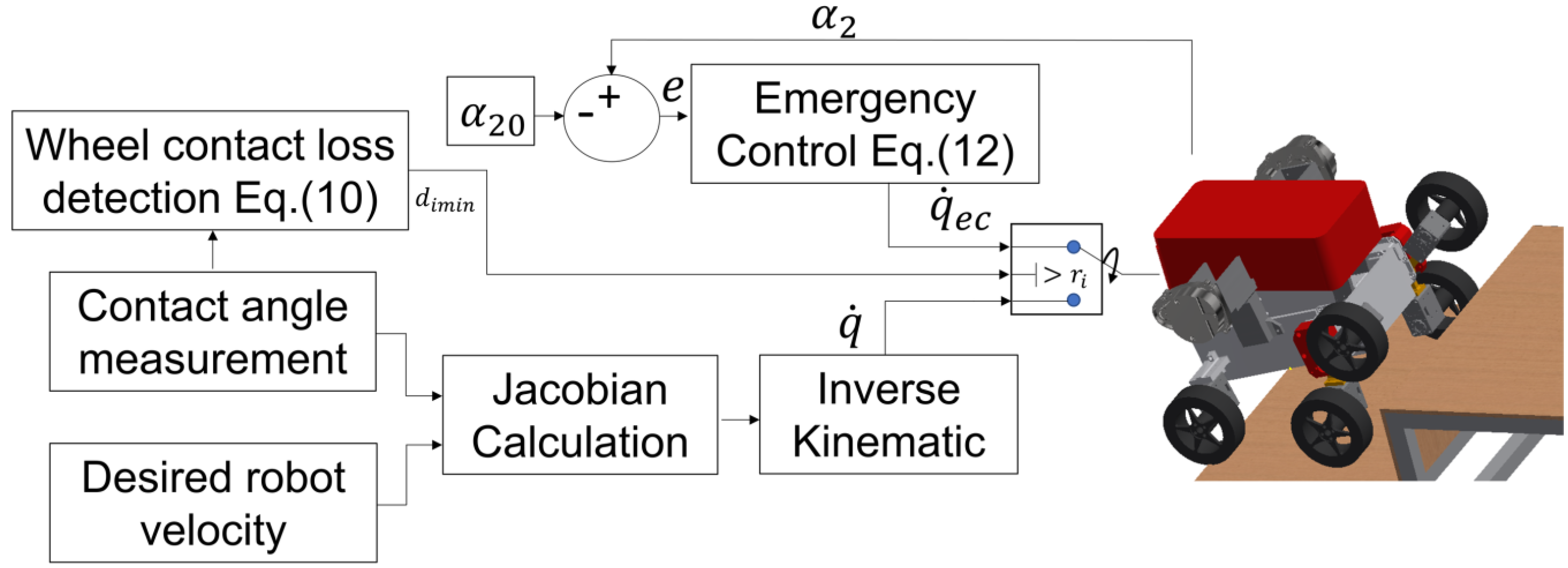
The next section details how the robot recognizes if it climbs up or down stairs. Additional emergency control prevents the robot from falling when the wheels lose contact with the ground.

3. Contact Angle Measurement and Emergency Control Based on Laser Scanning Sensor

The wheeled robot moves in different terrains, and it maintains stability while the wheels keep contact with the ground. The geometry of the terrain becomes essential information to adjust the wheel velocity according to surfaces such as ramps, holes, steps, and uneven terrain. The contact angle between the wheel and ground is a parameter to determine the terrain geometry. Therefore, we implemented the contact angle measurement using laser scanner sensors and the wheel-loss contact detection to prevent the robot from falling down the stairs using an emergency control.

3.1. Contact Angle between Wheel–Ground Using 2D Laser Sensors

The advantage of wheeled robots is their adaption to different terrains. However, when one of their wheels loses contact with the ground, they can lose their stability and fall. This section describes the method to measure the contact angle between the wheel–ground, which is a parameter of great importance to determine the terrain geometry. Thus, the robot can know if the wheels are touching a flat, vertical, sloped, or irregular surface. This way, we can implement an appropriate controller according to the terrain.

In previous research, the Jacobian and its inverse are calculated with the contact angle between the wheel–ground and the desired robot’s velocity [13]. There are some methods to measure or estimate the contact angle using internal and external sensors. The proposed method uses 2D laser sensors, that are easy to install, and precise measurement of terrain information. The LiDAR is installed on each side of the robot to scan the contact point between the wheel–ground and determine if the wheel loses contact with the ground, creating an emergency controller to avoid falls. The position from the LiDAR to the chassis is $l_6$; concerning the ground, it must be greater than 12 mm to guarantee the accuracy of the measurement $\pm 15$ mm. The sensor has a 1 degree range resolution and 360 degrees in total. The scanning range of each wheel is two times the diameter of each wheel to guarantee the measurement of the contact angle throughout the robot’s motion; otherwise, during climbing or descent, the information is lost.

Figure 9 shows the robot climbing a ladder, and the front wheel loses contact with the tread. The cyan color denotes the measurement of the front wheel, the pink color denotes the middle wheel, and blue denotes the rear wheel. $d_{imin}$, where $i=1,2,3$ in red color denotes the distance between the wheel center and contact point with the ground in Equation (5). $d_n$ denotes the distances of each degree n from the center of the wheel to the ground, and the minimum distance is $d_{imin}$. $l_r$ is the distance from the LiDAR to the wheel center, $l_n$ denotes the distances from the LiDAR to the ground, and ${\delta }_n$ is the angle between $l_n$ and $l_r$. Equation (6) calculates ${\varphi }_i$, the angle between $l_r$ and $d_{imin}$ inverse for each wheel.

$$min\left(d_n\right)=\sqrt{{l_r}^2+{l_n}^2-2l_r{l}_{n}cos\left({\delta }_{l_n}\right)}=d_{imin}$$

(5)

$${\varphi }_i={sin}^{-1}\left(\frac{d_{imin}sin\left({\delta }_i\right)}{\sqrt{{l_r}^2+{d_{imin}}^2-2l_r{d}_{imin}cos\left({\delta }_i\right)}}\right)$$

(6)

The contact angle measurement for the rear wheel ${\gamma }_3$ is given by Equation (7), where ${\theta }_3$ is a constant parameter defined by the angle between $l_r$ and $l_{rz}$, the vertical distance from the center of the rear wheel to the LiDAR. ${\alpha }_i$ is the angle formed by the inclination of the chassis, and ${\varphi }_3$ from Equation (6). The front and middle wheels depend on bogie rotation. The following variables are defined: $l_1$ and $l_2$ denote the distance between the bogie center and the front or middle wheel, respectively, $l_b$ is the distance between the LiDAR and the bogie. w denotes the angle between $l_b$ and the LiDAR z-axis, ${\lambda }_i$, where $i=1,2$ front and middle wheel is the angle between $l_b$ and $l_r$, ${\mu }_i$ denotes the angle between $l_b$ and $l_1$ or $l_2$ that varies by bogie rotation, ${\rho }_2$ is the angle between $l_r$ and the LiDAR z-axis by subtracting $\omega$ and ${\lambda }_i$. Finally, ${\varphi }_i$ is obtained from Equation (6). The contact angle measurement for the middle and the front wheel is given by ${\gamma }_2$ and ${\gamma }_1$ in Equations (8) and (9), respectively.

$${\gamma }_3={\varphi }_3+{\alpha }_i-{\theta }_3$$

(7)

$${\gamma }_2={\varphi }_2+{\alpha }_i+{\rho }_2$$

(8)

$${\gamma }_1=-{\varphi }_1+{\alpha }_i+{\rho }_1$$

(9)

The contact angles between the wheel–ground allow knowing the geometric surface. Thus, the velocity of each wheel can be adjusted according to the desired velocity of the robot’s center of mass in order to carry out a proper controller on different surfaces. For wheeled robots, we expect the wheels to maintain contact with the ground at all times to ensure stability; however, in reality, the wheels can lose contact with the ground and cause the robot to fall. Equation (10) determines if one of the wheels loses contact with the ground. $d_{imin}$ is the distance between the center of the wheel and the contact point measured with the laser sensor, and the wheel’s radius is the minimum distance $d_{imin}$ should have. Theoretically, 0 is the expected value to maintain contact with the surface, and any value greater than zero represents the distance moving away from the surface. The emergency controller is detailed in the following subsection when $d_{imin}$ is greater than zero.

$$d_{imin}-r_i>0$$

(10)

3.2. Emergency Controller to Prevent Robot Falls

In previous research, the Jacobian matrices of each wheel and its inverse were obtained [13]. The measurement of the contact angle between the wheel–ground using 2D laser sensors allows obtaining the geometric information of the terrain and detection of the wheel-contact loss. This information has an important role in preventing the robot from falling during climbing up or down. Figure 10 shows the schematic control of the wheeled robot, including the emergency control when a wheel loses contact with the ground. We set the desired robot velocity according to the contact angle measurement from the LiDAR. We calculated the Jacobian and its inverse to obtain the angular velocity of each wheel $\dot{q}={\left[w_1{w}_2{w}_3\right]}^T$, where $w_1$, $w_2$, and $w_3$ mean the angular velocity of the front, middle, and rear wheels, respectively. Therefore, the robot can follow the desired robot velocity.

The block “wheel-contact loss detection Equation (10)” defined an emergency case during climbing up or down stairs, the analysis focuses on the front wheel when it loses contact with the ground, which compromises the stability of the robot. When this case occurs, the switch changes the wheel’s velocity from the “inverse kinematic” block to the wheel’s velocity from the “Emergency Control Equation (12) ” block, ${\dot{q}}_{e}c={\left[w_{1ec}{w}_{2ec}{w}_{3ec}\right]}^T$, where $w_{1ec}$, $w_{2ec}$, and $w_{3ec}$ denote the front, middle, and rear wheel from the emergency control block. Thus, the controller stabilizes the robot until the wheel touches the ground and the switch changes again to the “inverse kinematic” block.

The emergency control kicks in when the first wheel detects the lost contact with the ground, the second wheel can lose contact, and the robot’s stability will not be compromised as long as the front and rear wheels are touching the floor. The parameter ${\alpha }_2$, Figure 3a,b is controlled, which is the angle between $l_2$ and the global horizontal axis Equation (11), $l_2$ is the distance between the center of the bogie and the middle wheel, ${\theta }_b$ is the rotation of the bogie, and ${\alpha }_{20}$ is the initial angle of ${\alpha }_2$ when the robot is on a flat surface. Suppose the front wheel loses contact with the ground, then, we want ${\alpha }_2$ to return its initial position ${\alpha }_{20}$ to prevent the robot falling. Therefore, ${\alpha }_{20}$ is a threshold in the controller, where e is the error control between ${\alpha }_2$ and ${\alpha }_{20}$, which it is the same as the bogie rotations ${\theta }_b$.

$${\alpha }_2={\alpha }_{20}+{\theta }_b$$

(11)

Based on the instantaneous center of rotation, Equation (12) includes the PD controller to adjust the velocity of the middle wheel. Thus, ${\alpha }_2$ reach the threshold ${\alpha }_{20}$; $w_b$, is the desired bogie velocity to achieve its ideal pose, then, the wheels’ velocities continue to use the Jacobian and its inverse matrix to follow the robot’s trajectory. The rear wheel during the emergency controller can inverse its velocity to maintain fixed the robot’s position until ${\alpha }_2$ reaches the initial position.

$${\dot{q}}_{ec}=\left[\begin{array}{c}{w}_1\\ w_b{l}_{2}sin({\alpha }_2+k_{p}e+k_d\dot{e})\\ -w_3\end{array}\right]$$

(12)

4. Simulation and Experiments

The 6-wheel robot was designed and optimized by the Taguchi method. Table 1 and Table 6 show the initial and optimized robot parameters. The simulation and experiments were carried out during climbing up and down steps of (6 × 17) cm, (7.5 × 25) cm, and (11 × 27) cm. The sensors for measuring the contact angle between the wheel–ground are encoders in each bogie, LiDAR sensor in each side of the robot, and IMU in the chassis. Each wheel has an independent actuator and one position-controlled motor in the chassis; To maintain the delivery package horizontal with respect to the ground, the IMU senses the rotation of the chassis. Then the motor rotates at the same angle in the opposite direction to the inclination of the chassis

Figure 11 shows the initial design (Figure 11a,b) and the optimal design using the Taguchi method (Figure 11c–f). The initial design can climb up stairs measuring (6 × 17) cm and (7 × 25) cm. However, The robot had problems while climbing up the stair measuring (11 × 27) cm, and during the robot’s descent, only the (6 × 17) cm step succeeded while the other two stairs resulted in falls; for that reason, we were motivated to optimize the robot design by the Taguchi method, then, we obtained the optimal parameters and created the new design. The optimal design can climb up the three stairs safely. However, climbing down (7 × 25) cm and (11 × 27) cm steps remains a problem due to the length of the robot from the front to the rear wheel being 28 cm, and based on the kinematic constraints to climbing down, the three wheels need to touch the step. Thus, the problem remains because the steps have 25 cm and 27 cm in length. Another solution is reduce the chassis length, which is 22 cm, but this parameter was not included in the Taguchi method because we cannot reduce the chassis space for the computer and sensors. Then, the emergency control helps the robot climb up and down safely without reducing the length of the chassis.

The case when emergency control work is when the front wheel loses contact with the ground. We detect this case using the contact angle method by the laser scanner sensor Equation (10). Figure 12 shows the contact angle between wheel–ground. The front, middle, and rear wheels are the lines colored cyan, magenta, and blue, respectively. In Figure 12a,b, the robot climbs up steps of (6 × 17) cm, in Figure 12c,d, the robot descends steps of (7.5 × 25) cm, and in Figure 12e,f, the robot descends steps of (11 × 27) cm. In Figure 12a,b, in simulation and experiment, it can be seen that the robot does not lose contact with the ground; for that reason, the lines are continuous. It can also be seen that when the robot is rising, the contact angle is 90 degrees. On the edges, it drops from 90 to 1 degree, and on the flat surface, it is zero degrees. Figure 12c–f) shows the descent of the robot on the (7.5 × 25) and (11 × 27) cm steps. The contact angle on the edge of the step goes up to 90 degrees, and when the wheel touches the vertical surface of the step, it is 90 degrees. The contact angle is zero when the wheel touches a flat surface or when it loses contact with the ground. In the second case, the emergency controller kicks in (Figure 13) when descending steps of (11 × 27) cm, where ${\alpha }_2$ denotes the angle between $l_2$ and the global horizontal axis, this is the parameter controlled to prevent the robot from falling. The threshold is ${\alpha }_{20}$ angle between $l_2$ and $l_4$, $d_{1min}$ is the distance the from the wheel to the ground, and the radius of the front wheel is $r_1$ and is the minimum value of $d_{1min}$ should prevent the wheel from moving away from the ground. When $d_{1min}$ is greater than $r_1$, the emergency controller acts, and it is activated by reducing the value of ${\alpha }_2$ to keep it at ${\alpha }_{20}$. Therefore, the robot maintains contact with the ground and descends safely. During climbing down the step of (11 × 27) cm, only in the first two steps, the front wheel loses contact with the ground, and we can see u is the control response to maintain ${\alpha }_2$ at the initial position.

The results of the robot climbing up and down stairs can be seen in the attached video https://youtu.be/NCi8Fp7Fl30, accessed on 15 April 2022.

5. Discussion

This paper shows the methodology design for wheeled robots to find optimal design parameters by considering kinematic constraints. An emergency control is also proposed to prevent the robot from falling when wheels lose contact with the ground, based on contact angle measurement and the wheel-contact loss detection using the LiDAR sensor. It is worth noting that the effectiveness of the measurement of the minimum distance $d_{imin}$ between the wheel and the ground depends on the LiDAR’s accuracy and the terrain profile. This paper considers rigid terrain because the robot moves in cities where the type of ground is concrete. Otherwise, errors can occur in diverse terrains such as grass, sand, and rocks, which compromises the system. Thus, the emergency control does not work appropriately. While in rigid terrain, the emergency control shows that the robot can climb up or down safely.

6. Conclusions

In this paper, the robot design was optimized by reducing the area between the trajectory of the CM of the delivery package and the slope of three different stairs using Taguchi’s method. The kinematic constraints of the wheeled robot were obtained. In addition, we found the maximum height step and the minimum length that the robot required to climb up and down. Thus, the robot can know if the obstacle is scalable. The emergency controller was also implemented to prevent the robot’s wheels losing contact with the ground, and the robot could climb safely. The information on the geometric terrain was obtained by measuring the contact angle using LiDAR sensors. The simulations and experiments validate the research carried out and the proposed method to recognize terrain geometry and the emergency controller to prevent the robot from falling from the stairs. The results obtained are detailed as follows:

• Robot design methodology for wheeled robots considering the kinematics constraints and the maximum height and minimum tread required to climb up or down stairs.
• Wheel-contact loss detection using laser scanner sensors.
• Implementation of emergency control to maintain the stability of the robot during ascent or descent of stairs.

In future works, we will include dynamic parameters in the robot design methodology, such as the weight of the wheels and the links to compensate the effect in a real test. We will also implement the contact angle measurement for uneven terrains with diverse profile terrains and the friction analysis between wheel–ground to create a torque control in scenarios where the robot is stuck or loses traction.

References

1. Jennings, D.; Figliozzi, M. Study of Sidewalk Autonomous Delivery Robots and Their Potential Impacts on Freight Efficiency and Travel. Transp. Res. Rec. 2019, 2673, 317–326. [Google Scholar] [CrossRef] [Green Version]
2. Hoffmann, T.; Prause, G. On the regulatory framework for last-mile delivery robots. Machines 2018, 6, 33. [Google Scholar] [CrossRef] [Green Version]
3. Patil, U.; Gujarathi, A.; Kulkarni, A.; Jain, A.; Malke, L.; Tekade, R.; Paigwar, K.; Chaturvedi, P. Deep Learning Based Stair Detection and Statistical Image Filtering for Autonomous Stair Climbing. In Proceedings of the 3rd IEEE International Conference on Robotic Computing, IRC 2019, Naples, Italy, 25–27 February 2019; pp. 159–166. [Google Scholar] [CrossRef]
4. Nguyen, P.T.T.; Yan, S.W.; Liao, J.F.; Kuo, C.H. Autonomous Mobile Robot Navigation in Sparse LiDAR Feature Environments. Appl. Sci. 2021, 11, 5963. [Google Scholar] [CrossRef]
5. Li, A.; Cao, J.; Li, S.; Huang, Z.; Wang, J.; Liu, G. Applied sciences Map Construction and Path Planning Method for a Mobile Robot Based on Multi-Sensor Information Fusion. Appl. Sci. 2022, 12, 2913. [Google Scholar] [CrossRef]
6. Nikpour, M.; Huang, L.; Al-Jumaily, A.M. An approach on velocity and stability control of a two-wheeled robotic wheelchair. Appl. Sci. 2020, 10, 6446. [Google Scholar] [CrossRef]
7. Li, X.; Liu, X.; Wang, G.; Han, S.; Shi, C. Applied sciences Cooperative Target Enclosing and Tracking Control with Obstacles Avoidance for Multiple Nonholonomic Mobile Robots. Appl. Sci. 2022, 12, 2876. [Google Scholar] [CrossRef]
8. Samsani, S.S.; Muhammad, M.S. Socially Compliant Robot Navigation in Crowded Environment by Human Behavior Resemblance Using Deep Reinforcement Learning. IEEE Robot. Autom. Lett. 2021, 6, 5223–5230. [Google Scholar] [CrossRef]
9. Sreenivasan, S.; Wilcox, B. Stability and traction control of an actively actuated micro-rover. J. Robot. Syst. 1994, 11, 487–502. [Google Scholar] [CrossRef]
10. Nagatani, K.; Ikeda, A.; Sato, K.; Yoshida, K. Accurate estimation of drawbar pull of wheeled mobile robots traversing sandy terrain using built-in force sensor array wheel. In Proceedings of the 2009 IEEE/RSJ International Conference on Intelligent Robots and Systems, IROS 2009, St. Louis, MO, USA, 11–15 October 2009; pp. 2373–2378. [Google Scholar] [CrossRef] [Green Version]
11. Frigola, M.; Casals, A.; Amat, J. Human–robot interaction based on a sensitive bumper skin. In Proceedings of the IEEE International Conference on Intelligent Robots and Systems, Beijing, China, 9–15 October 2006; pp. 283–287. [Google Scholar] [CrossRef]
12. Xu, H.; Liu, X.; Fu, H.; Putra, B.B.; He, L. Visual contact angle estimation and traction control for mobile robot in rough-terrain. J. Intell. Robot. Syst. Theory Appl. 2014, 74, 985–997. [Google Scholar] [CrossRef]
13. Pico, N.; Jung, H.R.; Medrano, J.; Abayebas, M.; Kim, D.Y. Climbing control of autonomous mobile robot with estimation of wheel slip and wheel-ground contact angle. J. Mech. Sci. Technol. 2022, 36, 959–968. [Google Scholar] [CrossRef]
14. Cevallos, H.; Intriago, G.; Plaza, D. Performance of the estimators weighted least square, extended kalman filter, and the particle filter in the dynamic estimation of state variables of electrical power systems. In Proceedings of the IEEE ICA-ACCA 2018—IEEE International Conference on Automation/23rd Congress of the Chilean Association of Automatic Control: Towards an Industry 4.0—Proceedings, Concepción, Chile, 17–19 October 2018; Volume 1, pp. 1–6. [Google Scholar] [CrossRef]
15. Shin, D.H.; Park, K.H. Velocity Kinematic Modeling for Wheeled Mobile Robots. In Proceedings of the IEEE International Conference Robotics Automation, CSeoul, Korea, 21–26 May 2001; Volume 4, pp. 3516–3522. [Google Scholar] [CrossRef]
16. Ge, P.; Wang, R. Velocity kinematics modeling and simulation for a lunar rover. In Proceedings of the 2010 International Conference on Electrical and Control Engineering, Wuhan, China, 25–27 June 2010; pp. 2519–2524. [Google Scholar]
17. Thueer, T.; Krebs, A.; Siegwart, R. Comprehensive locomotion performance evaluation of all-terrain robots. In Proceedings of the IEEE International Conference on Intelligent Robots and Systems, Beijing, China, 9–15 October 2006; pp. 4260–4265. [Google Scholar] [CrossRef] [Green Version]
18. Jiang, J.; Ding, G.; Zhang, J.; Zou, Y.; Qin, S. A Systematic Optimization Design Method for Complex Mechatronic Products Design and Development. Math. Probl. Eng. 2018, 2018, 3159637. [Google Scholar] [CrossRef] [Green Version]
19. Shabalina, K.; Sagitov, A.; Magid, E. Comparative analysis of mobile robot wheels design. In Proceedings of the 2018 11th International Conference on Developments in eSystems Engineering (DeSE), Cambridge, UK, 2–5 September 2018; pp. 175–179. [Google Scholar] [CrossRef]
20. Malmquist, D.; Frede, D.; Wikander, J. Holistic design methodology for mechatronic systems. J. Syst. Control Eng. 2014, 228, 741–757. [Google Scholar] [CrossRef]
21. Kim, N.; Bhalerao, I.; Han, D.; Yang, C.; Lee, H. Improving surface roughness of additively manufactured parts using a photopolymerization model and multi-objective particle swarm optimization. Appl. Sci. 2019, 9, 151. [Google Scholar] [CrossRef] [Green Version]
22. Rout, B.K.; Mittal, R.K. Parametric design optimization of 2-DOF R-R planar manipulator-A design of experiment approach. Robot. Comput. Integr. Manuf. 2008, 24, 239–248. [Google Scholar] [CrossRef]
23. Gjeldum, N.; Bilic, B.; Tomic, Z. Optimization of Chassis Design For Assembly Line Feeder Using Promethee and Taguchi Methods. In Proceedings of the 16th International Scientific Conference, Zagreb, Croatia, 8–10 June 2017; pp. 93–98. [Google Scholar]
24. Jeong, H.s.; Kim, T.k.; Kim, D.y.; Jung, B.j.; Song, H.j.; Lee, J.m.; Song, H.j. A Study on Driving Stability for Climb the Kerb of Outdoor Mobile Robot. In Proceedings of the 2020 The Korean Society of Mechanical Engineers Conference (2020), Online, 23–25 November 2020; pp. 1577–1578. [Google Scholar]
25. Hwang, J.H.; Kim, D.Y.; Kim, T.K.; Jung, B.J. Wheel Structure and Moving Body Using the Same to Overcome Obstacles. Korea Patent No. 10-2019-0167600, 10 December 2020. [Google Scholar] [CrossRef]
26. Nagendra, J.; Srinath, M.K.; Sujeeth, S.; Naresh, K.S.; Ganesha Prasad, M.S. Optimization of process parameters and evaluation of surface roughness for 3D printed nylon-aramid composite. Mater. Today Proc. 2021, 44, 674–682. [Google Scholar] [CrossRef]
27. Jeang, A.; Chung, C.P.; Ko, C.P. Optimizing Process Parameters on the LGP Molding Stamper through the Taguchi Method. IEEE Trans. Components Packag. Manuf. Technol. 2020, 10, 487–493. [Google Scholar] [CrossRef]
28. uz Zaman, U.K.; Boesch, E.; Siadat, A.; Rivette, M.; Baqai, A.A. Impact of fused deposition modeling (FDM) process parameters on strength of built parts using Taguchi’s design of experiments. Int. J. Adv. Manuf. Technol. 2019, 101, 1215–1226. [Google Scholar] [CrossRef]
Figure 1. CAD model design of a wheeled robot.
Applsci 12 04403 g001
Figure 2. 2D Schematic diagram of the wheeled robot.
Applsci 12 04403 g002
Figure 3. The maximum height the robot can climb up and down one step according to its kinematic constraints. (a) Prevents w 1 and w 2 climbing up or down together. (b) Prevents w 2 and w 3 climbing up or down together.
Applsci 12 04403 g003
Figure 4. Robot design methodology based on the Taguchi method.
Applsci 12 04403 g004
Figure 5. The trajectory of the wheels and the CM of the delivery package while the robot climbs one step of 11 × 27 cm.
Applsci 12 04403 g005
Figure 6. Sensitive analysis between control factors and S/N ratio.
Applsci 12 04403 g006
Figure 7. Second sensitive analysis between the control factors and S/N ratio.
Applsci 12 04403 g007
Figure 8. The area between the trajectory of the robot’s CM and the slope of the stairs while climbing up a step. (a,c,e) area of the initial design. (b,d,f) area of optimal design.
Applsci 12 04403 g008
Figure 9. Schematic 2D of the contact angle measurement and the loss of contact between wheel–ground using laser scanner sensors.
Applsci 12 04403 g009
Figure 10. Schematic of emergency control when the wheel loses contact with the ground.
Applsci 12 04403 g010
Figure 11. Simulation and experiment while climbing up and down stairs. (a,b) climbing up a step of (6 × 17) cm; (c,d) Climbing down a step of (7.5 × 25) cm; (e,f) climbing down a step of (11 × 27) cm.
Applsci 12 04403 g011
Figure 12. Contact angle measurement and the contact-loss detection between wheel–ground.
Applsci 12 04403 g012
Figure 13. Emergency control when the wheel loses contact with the ground, α 2 angle between l 2 and the global horizontal axis, u control of α 2 , α 20 threshold, d 1 m i n distance between the wheel center and the ground, and r 1 radius of the wheel and minimum distance of d 1 m i n to maintain wheel contact with the ground.
Applsci 12 04403 g013