A Few Shot Classification Methods Based on Multiscale Relational Networks

Abstract

Learning information from a single or a few samples is called few-shot learning. This learning method will solve deep learning’s dependence on a large sample. Deep learning achieves few-shot learning through meta-learning: “how to learn by using previous experience”. Therefore, this paper considers how the deep learning method uses meta-learning to learn and generalize from a small sample size in image classification. The main contents are as follows. Practicing learning in a wide range of tasks enables deep learning methods to use previous empirical knowledge. However, this method is subject to the quality of feature extraction and the selection of measurement methods supports set and the target set. Therefore, this paper designs a multi-scale relational network (MSRN) aiming at the above problems. The experimental results show that the simple design of the MSRN can achieve higher performance. Furthermore, it improves the accuracy of the datasets within fewer samples and alleviates the overfitting situation. However, to ensure that uniform measurement applies to all tasks, the few-shot classification based on metric learning must ensure the task set’s homologous distribution.

1. Introduction

Deep learning has made significant progress but still heavily depends on a large amount of annotated data [1,2,3,4]. Deep learning technology cannot perform well on new sample sets when lacking data. Inspired by humans’ ability to learn from small amounts of samples, researchers have increasingly studied the machines’ learning capabilities using a few samples, called few-shot learning. Thus, few-shot learning has become a significant frontier research focus in recent years.

The method aiming to learn from a single or a few samples is called small sample learning or few-shot learning [1]. It is based on the human ability to learn new concepts and obtain vibrant representations from little and sparse data. This ability mimics human’s realization and control over their learning process [5,6,7]. Few-shot learning considers new tasks using previous experience to learn quickly [8]. Therefore, it achieves the ability to learn “how to learn” [9,10]. It also solves the critical challenge of “categories or concepts vary from task to task” [11]. Research on this idea can be divided into the following aspects: the generation model using probabilistic reasoning and the discriminant model using meta-learning.

Li Fei-Fei et al. proposed the concept of small sample learning for the first time using generation models [12]. They proposed the Bayesian learning framework [13] in 2006. Then, Andrew L. Maas et al. proposed the Bayesian network to capture the attribute’s relationship, dealing with near-deterministic relations and soft probability relations [14]. In 2011, Brenden M. Lake et al. started to conduct studies on few-shot learning. They collected and produced an Omniglot data set suitable for few-shot learning and proposed a generation model of how characters are composed of strokes [15,16]. Next, a hierarchical Bayesian learning framework was proposed to solve learning with fewer samples for character recognition from the perspective of cognitive science [17,18]. Finally, the new deep generation model’s hierarchical Bayesian programming learning framework was proposed based on attention and feedback principles. In 2017, a probabilistic generation model named the Recursive Cortical Network can achieve the accuracy as the deep learning method with only one-millionth of the training samples. As a result, it can crack text captchas’ variants after one training [19].

In addition to generation models, the other popular option is meta-learning using previous experience when learning a new task. In 2016, Brenden M. Lake et al. emphasized it as the cornerstone of artificial intelligence [20]. The research directions for using meta-learning include the following: 1. memory enhancement; 2. measure learning; 3. learn the optimizer; 4. optimize initial characterization.

The memory or temporal convolution solves the over example problem in a cyclic network, called memory enhancement. It accumulates useful information in its external memory. In 2001, the memory-based neural network was proven to apply to meta-learning [21]. They adjusted the bias by updating the weight and adjusting the output by fast cache representation to the memory [22]. The neural network Turing machines use a different method to preserve different information. It uses external storage to store short-term information and apply slow weight updates for long-term ones [23]. Adam Santoro et al. proposed a memory enhancement network in 2017. The Long and Short Memory Network (LSTM) is the base for his new network [24]. Next, Munkhdalai et al. proposed a meta-learning network combined with a learning device and an added external memory unit called a meta-network [25].

Metric learning learns a similarity measure. It then compares and matches samples of new unknown categories. Specifically, input features are extracted by embedding functions. The input features are compared by simple distances, such as Euclidean distance and cosine distance [26]. Compared with the generated model, Gregory Koch’s twinned network does not include any additional prior knowledge about characters or strokes nor involves a complex reasoning process [26]. The model’s recognition accuracy on the Omniglot dataset is comparable to human results. In 2016, Oriol Vinyals’s end-to-end and optimized matching network used the memory and attention principle [1]. In 2017, Pranav Shyam et al. proposed using a recursion comparator based on an attention mechanism to solve a few-shot classification problem [27].

The learning optimizer is a program that learns the parameters of the learner, the updating function or the rules governing the new parameters. In the early studies on updating learner parameters using meta-learning, the most common method was to use network learning to modify its weight in multiple calculation steps on the input [28]. Studies on few-shot learning based on learning optimizers start from Sepp Hochreiter and Dougal Maclaurin et al. [23]. In 2017, Ravi and Larochelle adopted the LSTM meta-learner. They took the initial recognition parameters, learning rate, and loss gradient as the LSTM state. This structure improves the learning of its initialization parameters and the update rules [29]. Yang et al. proposed a meta-metric learner using Ravi’s meta-learner with metric learning [30]. The authors integrate the matching network and update rules with LSTM to obtain a better result. However, this structure is complex compared to those based only on measurement learning.

Optimizing the initial representation means optimizing the initial representation directly. In 2017, Chelsea Finn et al. proposed a model-agnostic meta-learning algorithm (MAML) [8]. Based on MAML, Zhenguo Denevi et al. regarded the learning rate as a learning vector [31]. They learned the optimizer’s initialization, updating direction, and learning rate in an end-to-end manner by using meta-learning. Compared with optimizing the initial characterization algorithm, this algorithm can make the learning appliance produce higher performance [31]. Liu et al. used the entire training set during the pre-train of the feature extractor. They captured useful parameters using the parameter generation model [32]. The metric learning image classification comprises feature extractors and measures learners [33,34]. The feature extractor extracts image features, and then the measure learner measures the distance between them. This method’s advantages and disadvantages lie in extracting better features and measuring the similarity between sets.

Since the performance of the method depends on the extraction and similarity measurements, this paper adopts a network form that could maximize the potential of these two sections. Therefore, this paper takes a multi-scale relational network (MSRN) to improve feature extraction and similarity measuring processes [35]. First, this paper introduces the two datasets used to train and test the new MSRN. Then, this paper provides a detailed explanation of the design of MSRN. When building MSRN, adding multi-scale features to the feature extractor improves the classification difference of extracted features. Secondly, the multi-scale feature combination of support and target sets is designed. Finally, the similarity of support and target sets is learned using the relational network [36,37], and the neural network measures learners. After providing all the proposed method results and the three comparison methods, the paper discusses the novelty and limitations of MSRN while providing future research suggestions regarding them.

2. Materials and Methods

Two datasets are selected, the Omniglot dataset and the MiniImageNet dataset, to evaluate and examine the performance and accuracy of the proposed method. The two datasets are briefly introduced below.

By using Amazon’s Mechanical Turk, Brenden Lake et al. at MIT collected and published the Omniglot data set [20]. It comprises 50 international languages. The letters in each language vary widely, as shown in Figure 1. Therefore, the Omniglot dataset consists of 32,460 images from 1623 categories.

The MiniImageNet dataset consists of 60,000 84 × 84 × 3 color images. This dataset produced by Vinyals et al. has 100 categories and 600 samples in every category [1]. The dataset’s distribution is different from Omniglot. The image category involves animals, goods, and remote sensing photos. This original dataset is not published. Ravi and Larochelle produced and published the MiniImageNet dataset by randomly selecting 100 classes from the ImageNet. This new set is divided into training, validation, and test sets at 64:16:20 [29].

The few-shot image classification methods based on metric learning include four types of networks. By learning similarity measurements from various tasks, metric learning guides new tasks using experience extracted from previous tasks. First, the learner learns from the training tasks by measuring the support set’s distance and learns a metric. Then, a small number of support set samples can correctly classify the target set for the test set’s new task.

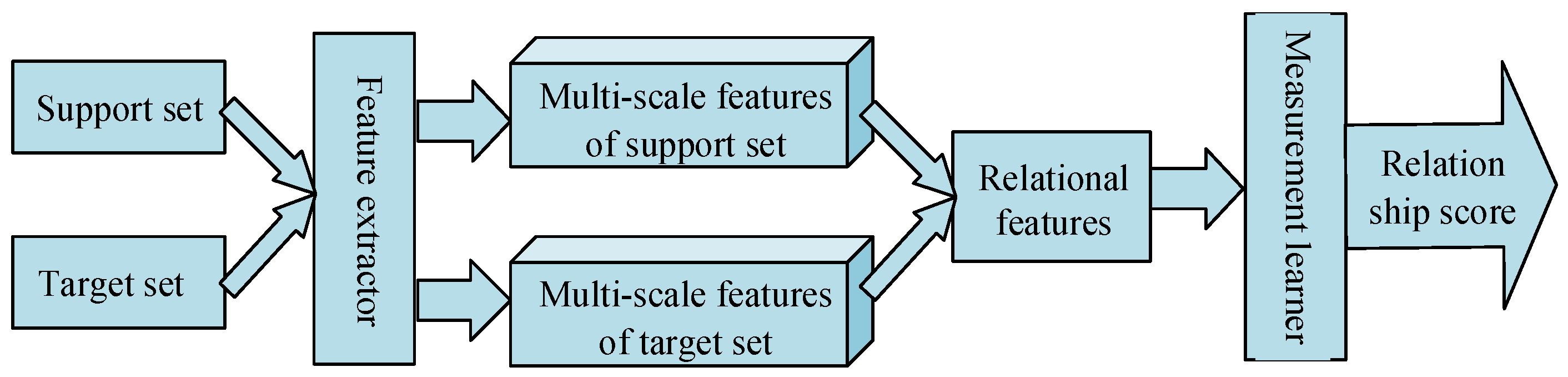
This paper aims to calculate two images’ similarities using the support and target sets. The three types of metric learning networks (the matching, the prototype, and the relational) are selected in comparing experimental results. The network design of the proposed multi-scale relational network (MSRN) is shown below.

2.1. Structural Design of Multi-Scale Relational Network

The structure of the multi-scale relational network is shown in Figure 2.

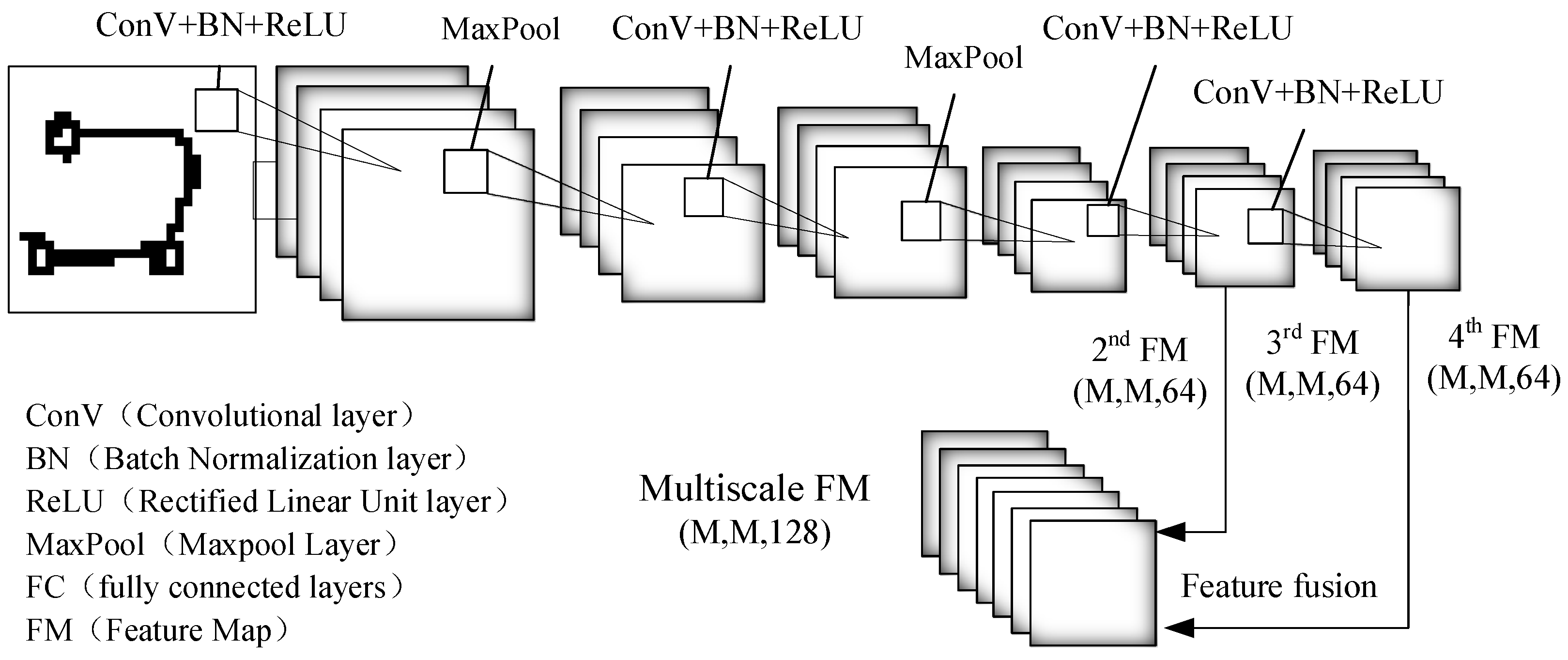
Like the matching network, our MSRN adopts a four-layer Convolution Neural Network (CNN) with the fully connected layer removed as the feature extractor [33,34,38]. For feature extractors composed of four layers of convolution, twenty-four or thirty-four layers of features are mainly considered. The specific structure of the feature extractor is shown in Figure 3.

MSRN combines the samples’ multi-scale features of each category of the supporting set with those of the target set. Finding the mean is the same as extracting the central point of each type of supporting set in the prototype network. Finally, we obtain a support set prototype with multi-scale characteristics.

Like relational networks [39], MSRNs use a network to learn the similarity between features. The metric learner’s specific structure is shown in Figure 4, composed of two convolution modules and two fully connected layers. The Rectified Linear Unit (ReLU) activation function is used in the first layer. The sigmoid activation function is used in the second layer. The two activation functions are selected according to the ability to improve the computational speed and the capacity to perform complex decisions [40,41].

It formulates an MSRN, as shown below:

$$\begin{gathered} {\overline{x}}_n^i=f_{\phi }\left(x_n^i\right), {\overline{x}}_n^j=f_{\phi }\left(x_n^j\right),{\overline{x}}_{\overline{n}}=\frac{1}{k}{\displaystyle \sum }_{i=1}^k{\overline{x}}_n^i \\ {r}_{\overline{n}j}=g_{\varphi }\left(\left|{\overline{x}}_{\overline{n}}-{\overline{x}}_n^j\right|\right),{\overline{y}}_n^j=\max \left(r_{\overline{n}j}\right) \\ i=1,\dots ,k; j=1,\dots ,b; n=1,\dots ,N; \overline{n}=1,\dots ,N \end{gathered}$$

(1)

where $f_{\phi }\left(x\right)$ represents feature extractor; $g_{\varphi }\left(\overline{x}\right)$ stands for measurement learner; $x_n^i$ and $x_n^j$ represent the original pixel features of the sample images of the support set and the target set; and ${\overline{x}}_n^i$ and ${\overline{x}}_n^j$ represent the multi-scale characteristics of support set and target set samples. ${\overline{x}}_{\overline{n}}$ represents the prototype of each type of sample of the supporting set. |…| represents the absolute value of the 3D vector after direct subtraction. $r_{\overline{n}j}$ is the relational score. ${\overline{y}}_n^j$ represents the prediction label of the target set sample.

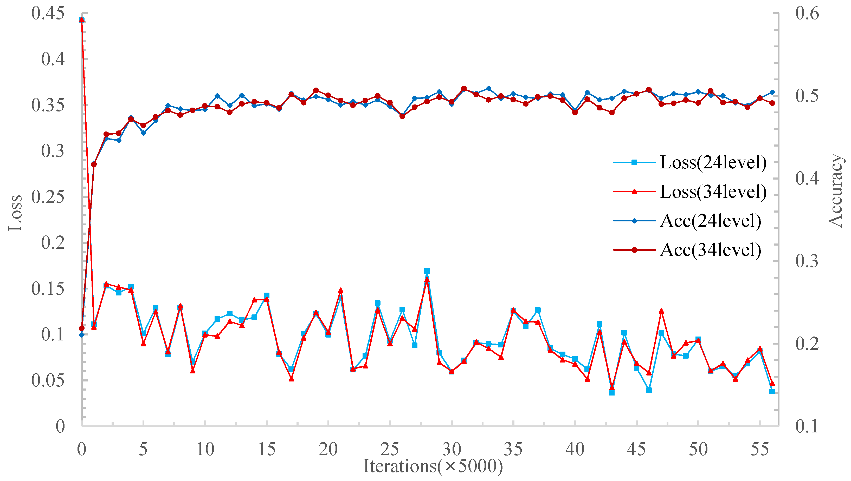
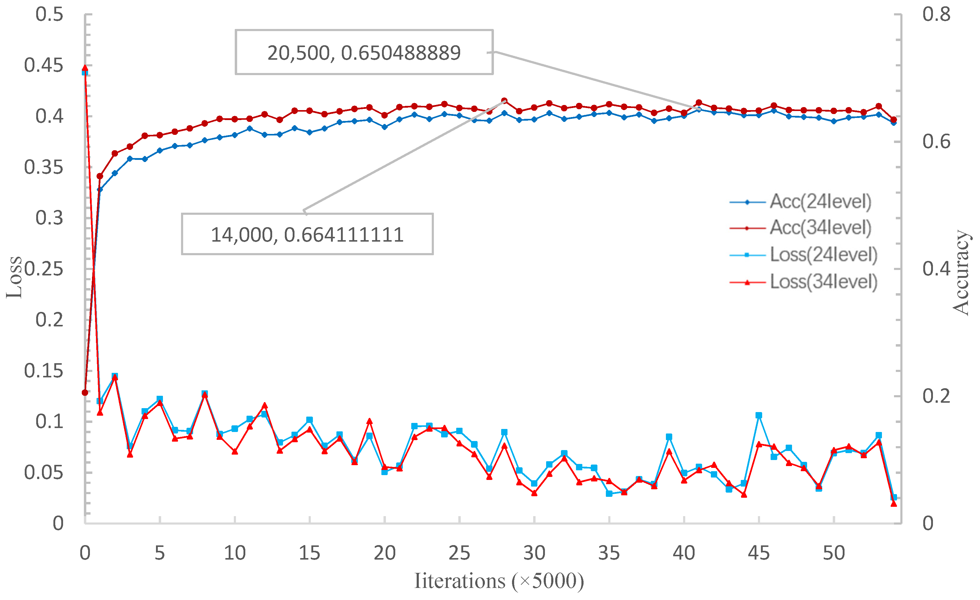
The 24-layer and 34-layer features were combined to conduct 5W1S and 5W5S experiments on the miniImageNet set. The experimental results are shown in Figure 5 and Figure 6.

Combined with the experimental results and considering the adaptability of more data, the MSRN selected 34 layer features as multi-scale features after stitching them together in the depth direction.

The test results of the single-sample classification experiment of 5W1S on the miniImageNet data set are shown in

Table 1. Classification results with a 95% confidence interval of single sample images.

	Single Scale Characteristic	Multi-Scale Characteristic (5-Way 5-Shot with Small Samples)
Three-dimensional splicing	50.16 ± 1.34%	51.1 ± 0.97% (64.70 ± 0.61%)
Three-dimensional subtraction	49.45 ± 1.28%	50.21 ± 1.08% (65.89 ± 0.32%)

. The data in brackets are the results of the image classification experiment 5W5S with small samples. The three-dimensional subtraction stitching method is chosen with experimental results and consideration.

2.2. Multi-Scale Relational Network Learning

MSRN completes the regression task. Therefore, the mean square error calculates the predicted distribution distance and the expected probability distribution [39]. The specific calculation formula of mean square error is as follows:

$$\phi ,\varphi \leftarrow arg \underset{\phi ,\varphi }{min}{{\displaystyle \sum }}_{\overline{n}=1}^N{{\displaystyle \sum }}_{j=1}^{n_T}{(r_{\overline{n}j}-1(y_{\overline{n}}=={\overline{y}}_n^j))}^2$$

(2)

where $\phi$ represents the feature extractor parameter, and $\varphi$ represents the measurement learner parameter. argmin refers to the extraction of the values of $\phi$ and $\varphi$ when the following formula reaches the minimum value. $n_T=N\times b$ represents the total number of image samples of the target set. $y_{\overline{n}}$ is the label supporting each category of the set. ${\overline{y}}_n^j$ is the prediction label for the image sample of the target set. The similarity of the same matching pair is 1, and the similarity of different matching pairs is 0. $r_{\overline{n}j}$ can be calculated from Equation (1).

An MSRN is an end-to-end differentiable structure. Backpropagation algorithm [42] and adaptive moment estimation [43] are adopted to adjust the parameters’ value.

During training, after the end of an EPOCH (After completing epoch different task training), the accuracy on the verification set was calculated, and the highest result was recorded. When 30 consecutive epochs (or more, adjusted for specific conditions) were not optimal, the accuracy was deemed to have stopped improving. After the accuracy stops improving or starts decreasing, the iteration can be stopped. First, the model corresponding to the highest accuracy can be output, and then the model can be tested [39]. The calculation formula of accuracy is as follows:

$$\mathrm{accuracy}=\frac{1}{n_T\times episode}{{\displaystyle \sum }}_{k=1}^{episode}{{\displaystyle \sum }}_{n=1}^N{{\displaystyle \sum }}_{j=1}^b\left({\overline{y}}_n^j=y_n^j\right)$$

(3)

where episode represents the number of tasks, and one task is image classification with a few samples. $n_T$ represents the total number of samples on the target set. ${\overline{y}}_n^j$ represents the predicted tag value of the target set sample, and $y_n^j$ represents the tag value of the target set sample. $b$ represents the value of each type of image in the target set, namely the batch number. N represents the sample categories in a few shot image classification tasks.

3. Results

All samples were processed into a size of 28 × 28. A rotation for enhancement was performed, and 1200, 211, and 212 were randomly selected as training, verification, and test sets. In addition, this paper conducts single-sample experiments of 5-ways 1-shot (5W1S) and 20-ways 1-shot (20W1S) and small-sample experiments of 5-ways 5-shot (5W5S) and 20-ways 5-shot (20W5S).

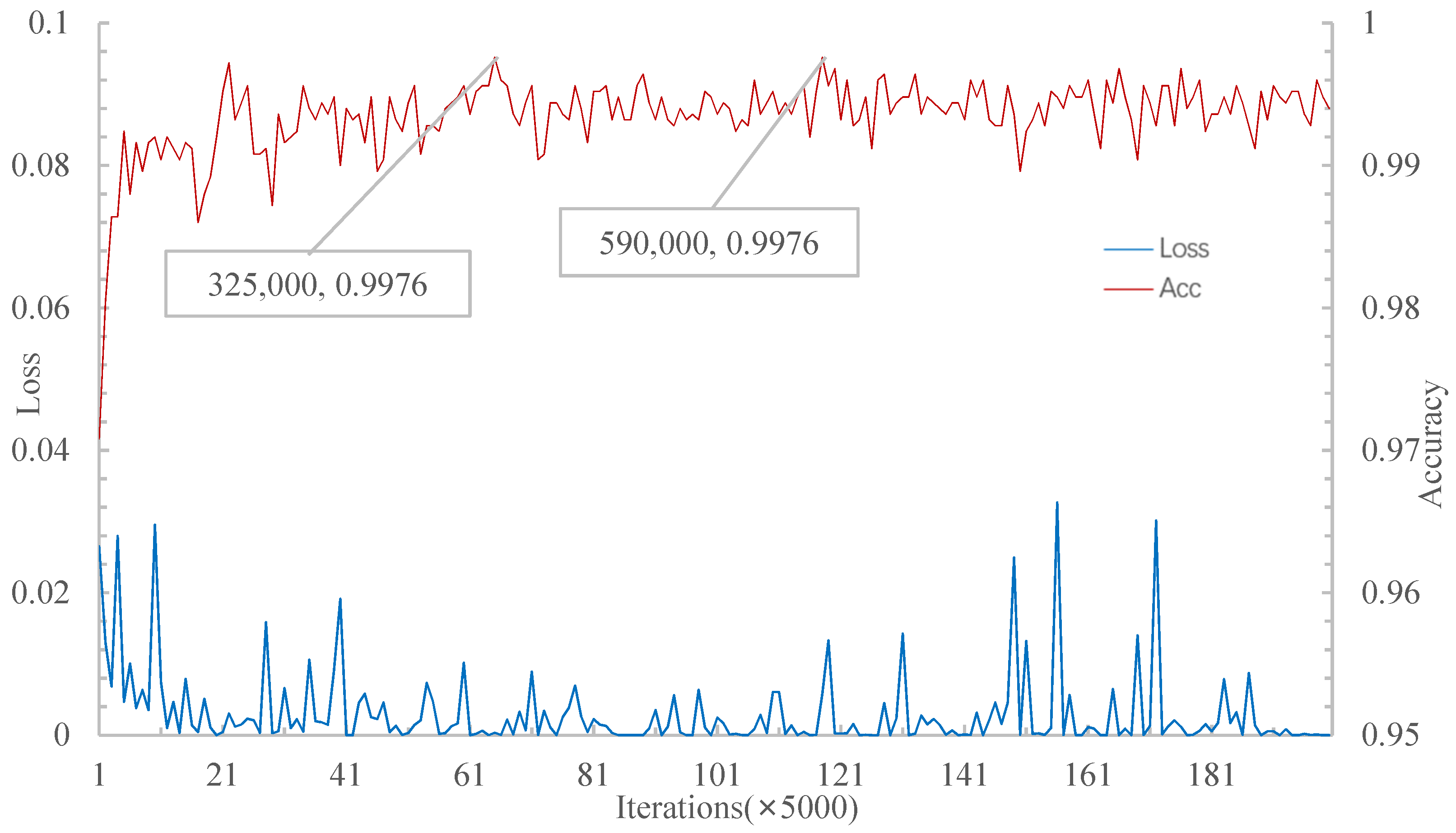
Figure 7 shows that the network achieved the highest accuracy of 99.76% in the 5W1S experiment when the number of iterations was 325,000. Figure 8 shows that MSRN achieves the highest accuracy of 99.72% in the 5W1S experiment on the verification set when the number of iterations is 114,000.

Therefore, for the 5W1S experiment, MSRN converges to the highest accuracy faster than the relational network. However, the highest accuracy on the verification set is slightly lower than the relational network. The trained model is tested on the test set, and the results are shown in

Table 2. Experimental results of few-shot classification of Omniglot data set.

Model	Fine-Tuning	Accuracy (95% Convidence Interval)
		5-Way 1-Shot	20-Way 1-Shot
The Matching network	No	98.10 ± 0.23%	93.80 ± 0.33%
The Prototype network	No	98.80 ± 0.12%	96.00 ± 0.28%
The Relational network	No	99.32 ± 0.16%	96.73 ± 0.15%
The Multi-scale relational network	No	99.35 ± 0.25%	97.41 ± 0.28%

with a 95% confidence interval. The accuracy rate of the MSRN in the 5W1S experiment on the test set is higher than that of the other three methods.

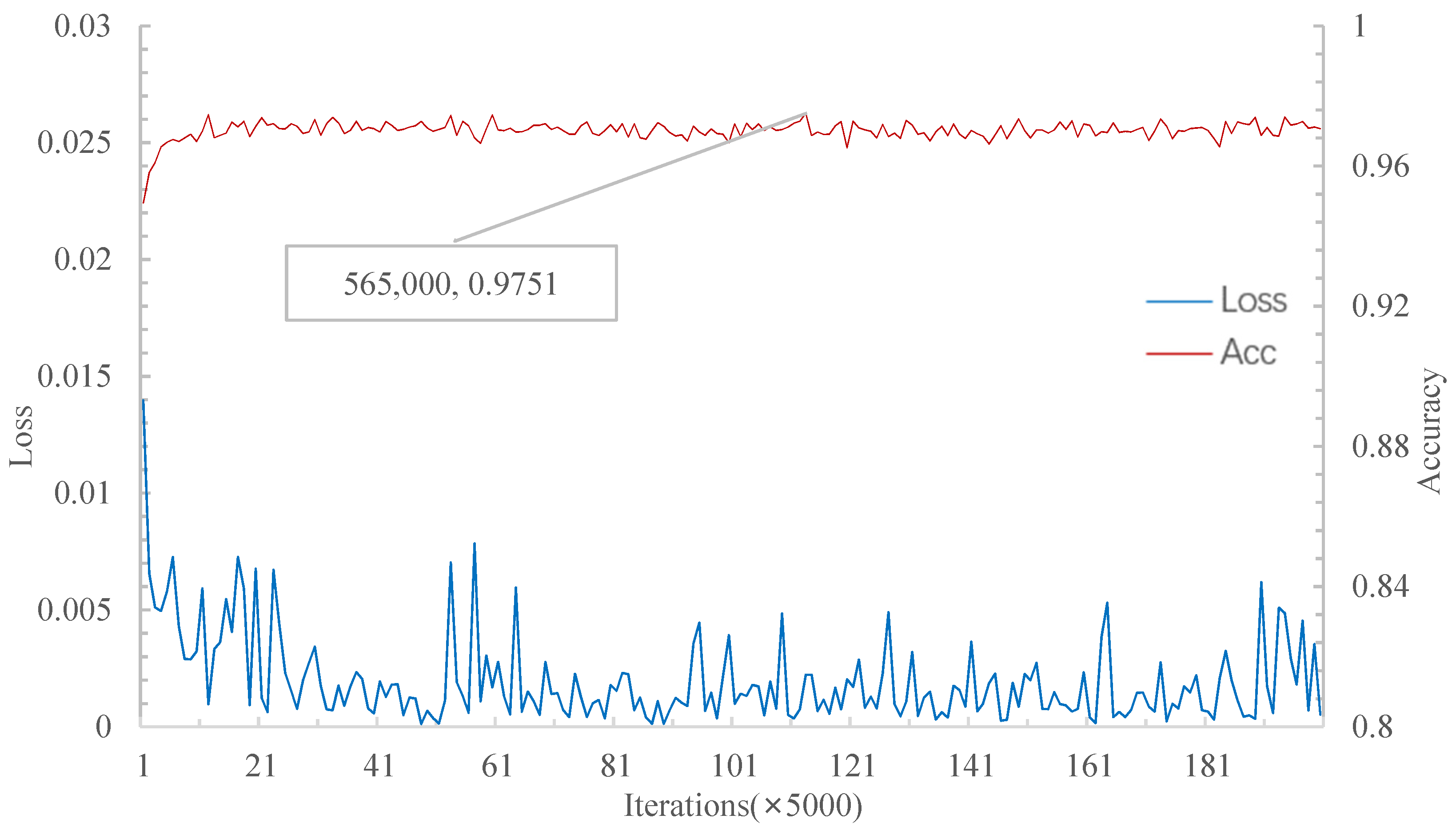
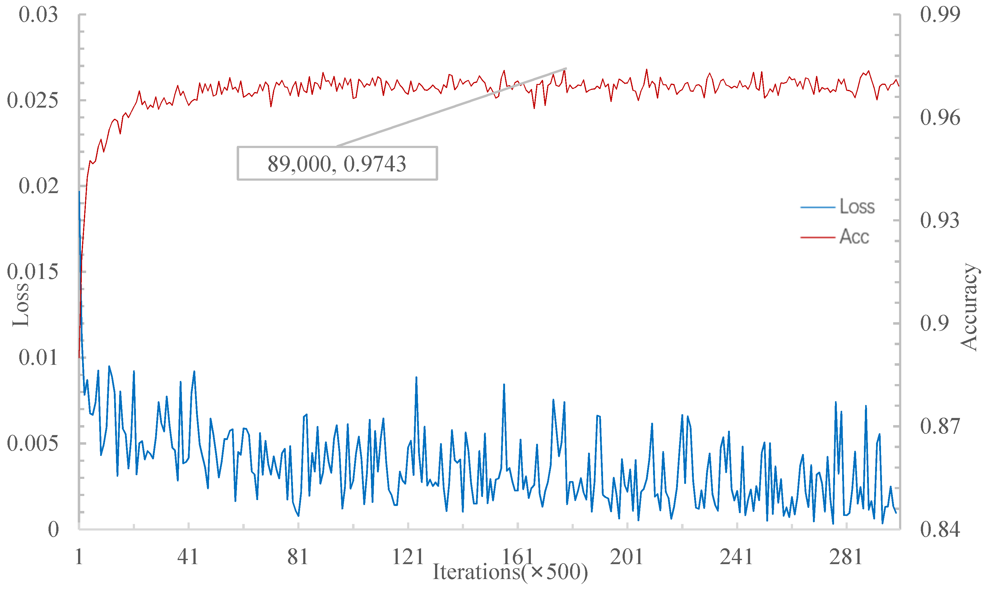
In Figure 9, when the iterations achieve 565,000, the relational network has the highest accuracy of 97.51% in the 20W1S experiment. On the other hand, as shown in Figure 10, when the iteration is 89,000, MSRN achieves 97.43% accuracy (highest) in the 20W1S experiment. Therefore, for the 20W1S experiment, although the highest accuracy rate of the relational network is higher than that of the MSRN, MSRN converges to the highest accuracy much faster. As shown in Table 2, the accuracy rate of the 20W1S experiment on the test set of the MSRN is higher than that of the matching network, the prototype network, and the relational network.

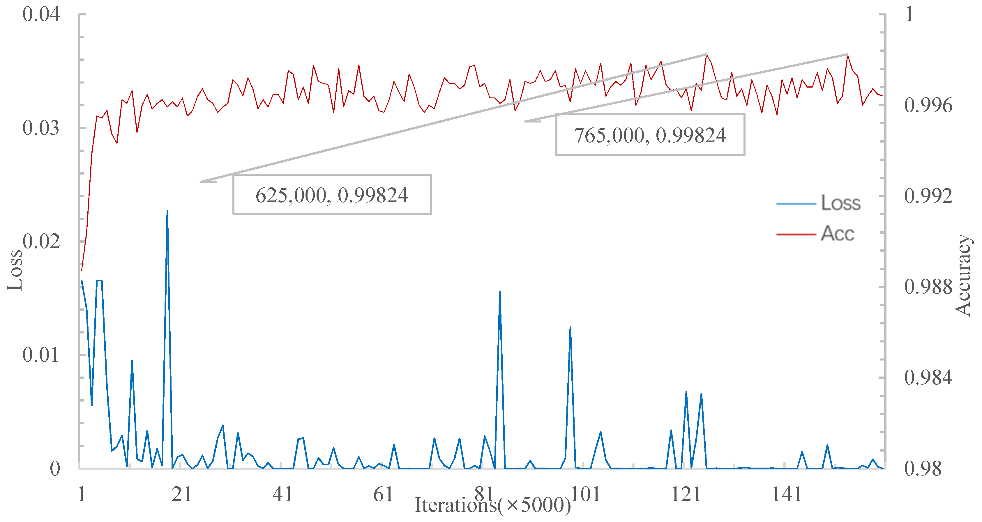
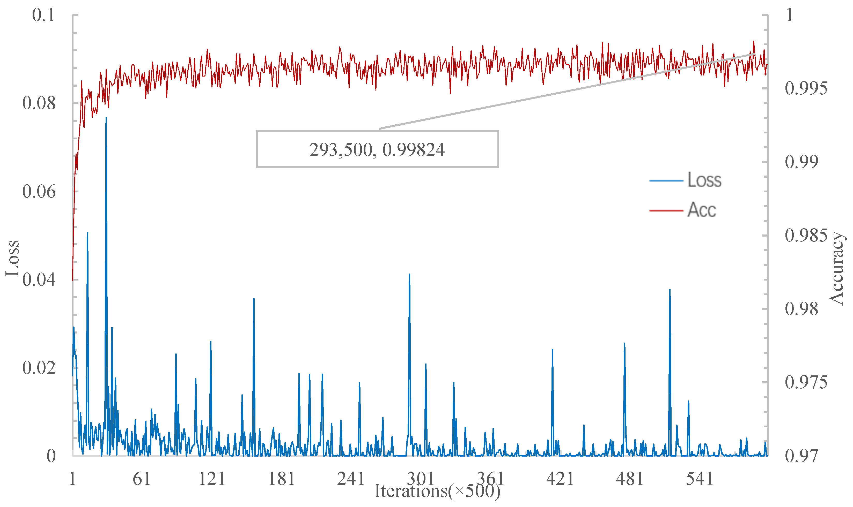
Figure 11 shows that when iterations achieve 625,000, the relational network has the highest accuracy of the 5W5S experiment at 99.824%. Figure 12 shows that when the iteration reaches 293,500, the MSRN (the method in this paper) achieves the highest accuracy of 99.824% in the 5W5S experiment.

Therefore, for the 5W5S experiment, the relational network’s highest accuracy rate on the verification set is similar to that of MSRN. However, MSRN converges to the highest accuracy rate faster than the relational network. The trained model is tested on the test set, and the results with a 95% confidence interval are shown in

Table 3. Experimental results of few-shot classification of Omniglot data set.

Model	Fine-Tunning	Accuracy (95% Convidence Interval)
		5-Way 5-Shot	20-Way 5-Shot
Matching network	No	98.90 ± 0.32%	98.50 ± 0.18%
Prototype network	No	99.58 ± 0.45%	97.60 ± 0.10%
Relational network	No	99.64 ± 0.09%	98.91 ± 0.05%
Multi-scale relational network	No	99.70 ± 0.08%	99.01 ± 0.13%

. The accuracy rate of the 5W5S experiment on the test set of the MSRN is higher than that of the matching network, the prototype network, and the relational network.

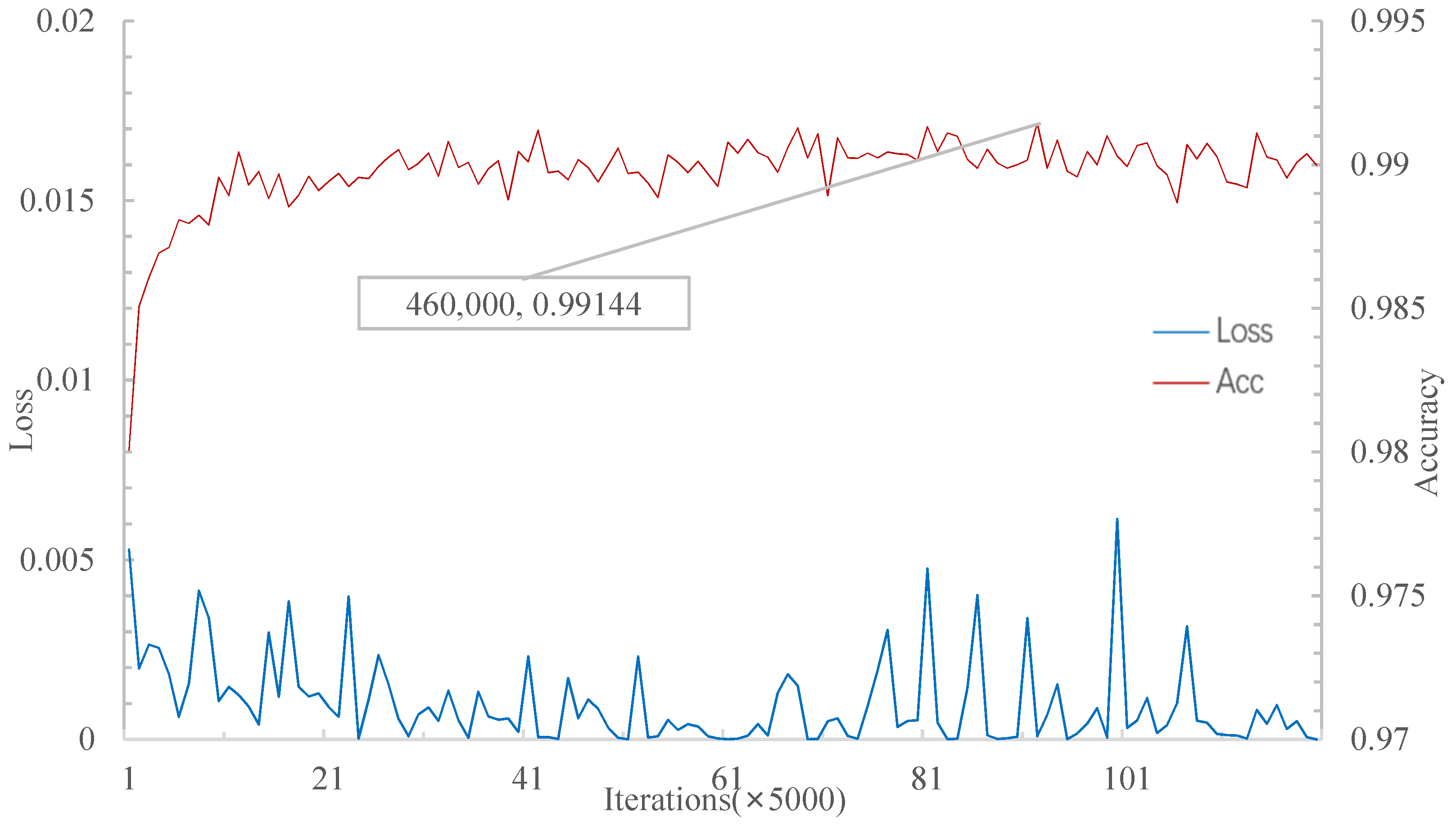
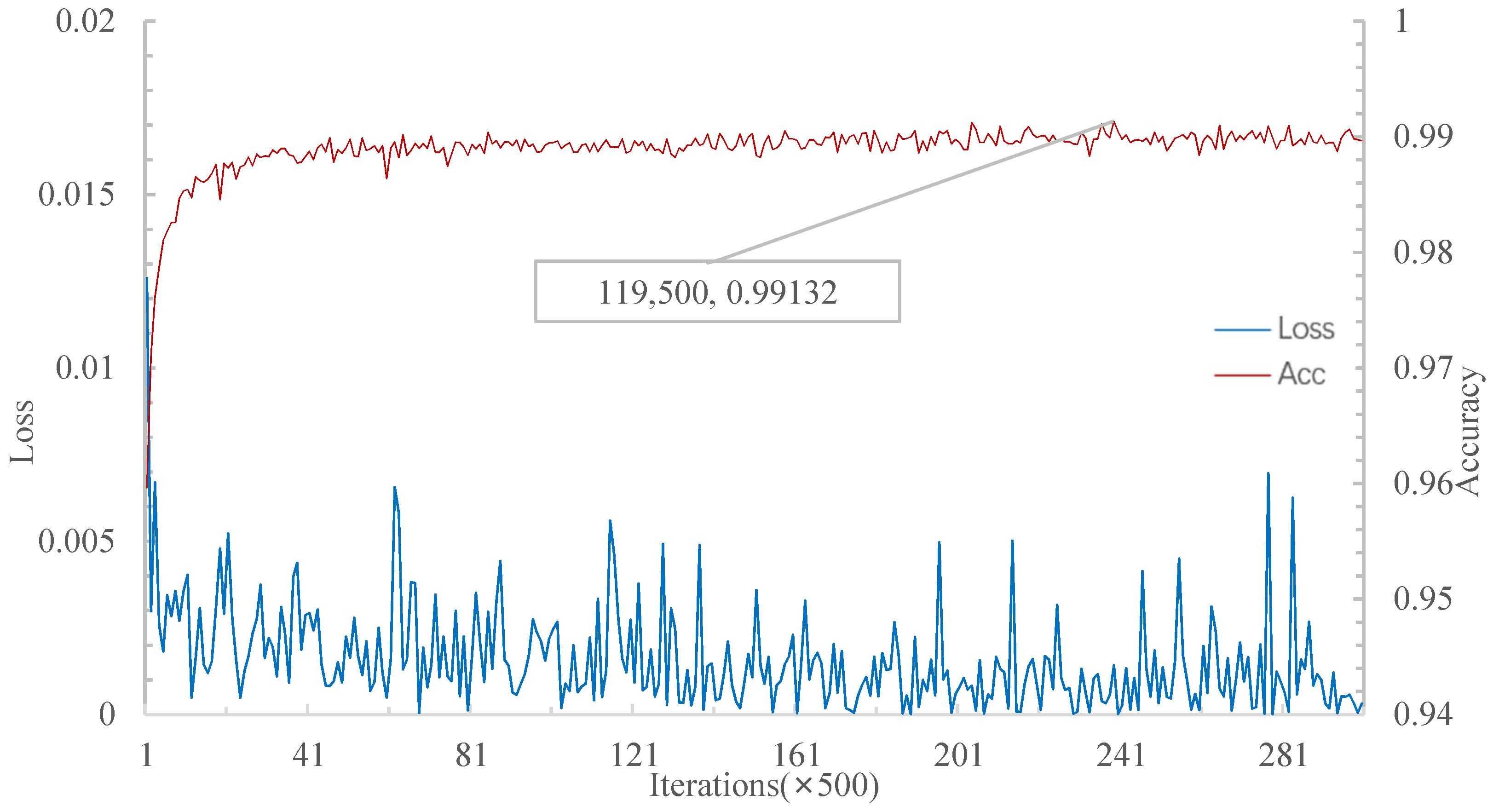
Figure 13 shows that when iterations achieve 460,000, the relational network has the highest accuracy of 99.144% in the 20W5S experiment. In Figure 14, MSRN achieves 99.132% accuracy in the 20W5S experiment at 119,500 iterations.

For the 20W5S experiment, the relational network’s highest accuracy rate is higher than MSRN. However, MSRN is faster than the relational network in the convergence rate. In Table 3, the accuracy rate of the MSRN is higher than that of the matching network, the prototype network, and the relational network.

According to the data set production method of Ravi and Larochelle, this section conducts the single-sample image classification experiment of 5W1S and the small-sample image classification experiment of 5W5S.

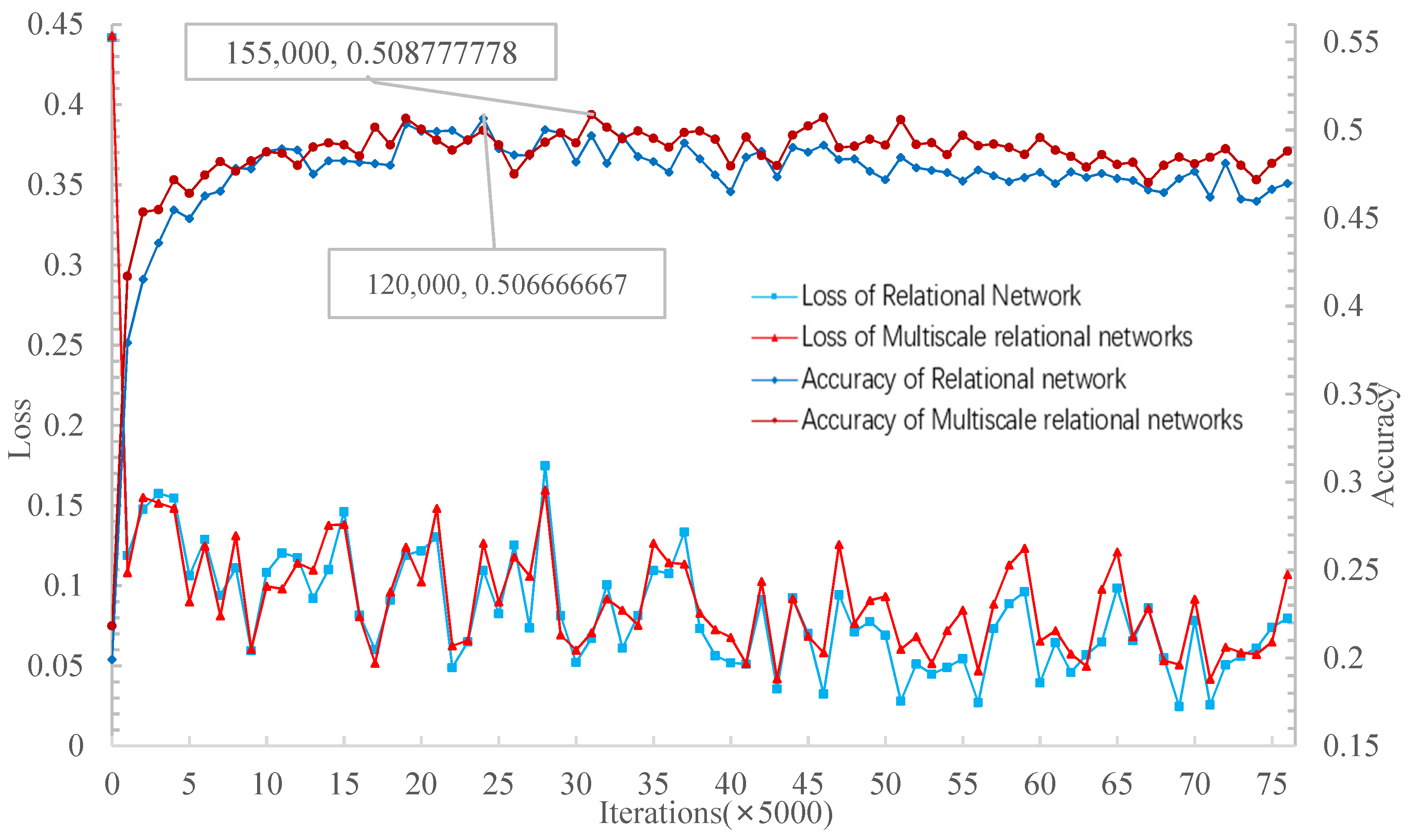
Figure 15 shows that when the number of iterations is 120,000, the network achieves the highest accuracy of 50.67% in the 5W1S experiment. On the other hand, the proposed method achieved the highest accuracy of 50.87% with 155,000 iterations. Therefore, for the 5W1S experiment, the relational network’s convergence rate to the highest accuracy is faster than the MSRN. However, the highest accuracy on the verification set is slightly lower than that of the MSRN.

Figure 15 shows that after the relational network converges to the highest accuracy, the loss decreases when the accuracy slowly decreases with iteration increases. However, the loss is close to convergence when the multi-scale relation network converges to the highest accuracy. With iteration increases, the loss decreases to convergence, and the accuracy tends to be stable. After the loss converges, the accuracy slowly decreases with iteration increases. The trained model is tested on the test set, and the results with a 95% confidence interval are shown in

Table 4. Results of the 20-way 5-shot on the MiniImageNet data set.

Model	Fine Tunning	Accuracy (95% Confidence Interval)
The Matching network	No	43.27 ± 0.96%
The Prototype network	No	49.35 ± 0.67%
The Relational network	No	50.16 ± 1.34%
The Multi-scale relational network	No	50.21 ± 1.08%

. The accuracy of the 5W1S experiment on the MSRN test is higher than that of the other three methods.

Figure 16 shows that when the iteration reaches 55,000, the relational network achieves the highest accuracy of 65.23% in the 5W5S experiment. On the other hand, when the number of iterations is 140,000, the proposed method achieves the highest accuracy rate of 66.41% in the 5W5S experiment. Therefore, for the 5W5S experiment, the relational network’s convergence rate to the highest accuracy is faster than MSRN. However, the highest accuracy on the verification set is slightly lower than that of the proposed method.

Figure 16 shows that, with the 5W1S experiment, after the relational network converges to the highest accuracy rate, with the increases in iteration, the accuracy also slowly decreases when the loss continues to decline. However, the loss is close to convergence when the multi-scale relation network converges to the highest accuracy. With the iteration increase, the loss and accuracy tend to be stable. The trained model is tested on the test set, and the results are shown in

Table 5. Results of the 5-way 5-shot on the miniImageNet data set.

Model	Fine Tunning	Accuracy (95% Confidence Interval)
Matching network	No	55.16 ± 0.64%
Prototype network	No	68.15 ± 0.77%
Relational network	No	64.77 ± 0.34%
Multi-scale relational network	No	65.89 ± 0.32%

with a 95% confidence interval. The accuracy rate of the 5W5S experiment on the MSRN test set is higher than that of the relational network and matching network but lower than that of the prototype network.

4. Discussion

By conducting the proposed learning on a wide range of tasks, the multi-scale network can effectively use the learning experience in the previous task, realizing learning to learn. For example, the network can classify images that it had never seen with only a small sample of the new categories.

The multi-scale features capture a clear class difference compared to those of the single-scale. Compared to the fixed measure, the learning measure shows more flexibility. Moreover, the multi-scale features can better capture the differences’ characteristics than other methods. Hence, the proposed multi-scale network shows higher classified accuracy in most experiments than the relationship network, the matching network, and the prototype network.

On the other hand, it has a lower accuracy than the prototype network on the 5-way 5-shot experiment on the miniImageNet dataset. MSRN also improves the Omniglot data set’s training speed compared with the relational network.

Under the scenario setting of meta-learning, the learning process can continue forever, thus realizing lifelong learning. When the relational network converges to the highest accuracy rate, with the increase in iteration, the loss continues to decrease while accuracy also decreases slowly. However, the loss of the MSRN proposed in this paper converges after achieving the highest accuracy. With the iteration increase, the loss and accuracy tend to be stable.

Therefore, we regard the improvement of classification accuracy as a learning process. Unfortunately, with the increasing number of learning tasks (iteration times), the relational network’s learning process on the miniImageNet data set could not continue. However, because the multi-scale feature combination method proposed in this paper can prolong the learning process by taking the absolute value after subtracting two features, the multi-scale network alleviates the overfitting phenomenon on the miniImageNet data set. Compared with the miniImageNet data set results, those on the Omniglot data set showed a slight difference in distribution, a good learning effect, and a much higher accuracy rate.

5. Conclusions

This paper designs a new MSRN. By measuring learning on a wide range of tasks, this method can use previous experience to learn how to learn. Furthermore, it realizes deep learning methods to quickly learn and generalize from a small number of sample images. 1. The MSRN will remove the fully connected layer of the four-layer CNN and stitch the 34-layer feature maps in the depth direction to obtain multi-scale features. The MSRN calculates the mean value of the multi-scale features of each category of the supporting samples. It then combines the multi-scale features of the target set samples to take the absolute value after subtracting the elements to obtain the relational features. The network then learns the relational features through the neural network.

This method is simple and effective, which improves the classification difference of feature extraction. The classification accuracy on the baseline set of few-shot learning is improved with multi-scale feature subtraction between the supporting and target sets. The overfitting of the training on the miniImageNet dataset is also alleviated.

Although the method in this paper improves the classification accuracy on the benchmark set with few samples and the overfitting situation, it still needs to be improved in the following aspects:

Compared with the miniImageNet data sets, the Omniglot dataset is less complicated. The Omniglot baseline accuracy is above 97% on the few-shot learning problems, but on the miniImageNet data set, the classification effect still needs improvement. Although it was improved compared to past methods, this method still cannot capture the feature when performed on a complex dataset. Along with the complex network design, the structure of this method could be further improved. Future studies could focus on finding other meta-learning methods to improve the ability to identify the critical features of complex data.

Under the limited experiment settings, the proposed method has demonstrated its advantage. The effectiveness of MSRNs also indicates that simple design choices can achieve the same or higher performance. However, multi-level features are deeply splicing. Due to the influence of high-level feature similarity, the low-level feature similarity needs to be improved to distinguish fine granularity differences. In this paper, multi-scale features are extracted and combined using a relatively shallow model. It is limited to completing the combination and screening of complex information. The proposed network is based on a well-established method and structured into a multi-scale network in a relatively straightforward manner. This structure means that even though it is an improved method, it still suffers many drawbacks of the base networks such as those from CNN and the fully connected layer. Suppose that it can be combined with other networks or meta-learning methods and the Bayesian model. In that case, it is believed that more significant breakthroughs will be made, and the ability to draw fertile conclusions will be more robust.