Research on Damage Localization of Steel Truss–Concrete Composite Beam Based on Digital Orthoimage

Featured Application

Holographic deformation data of a bridge structure can be obtained from the image data, and areas with excessive structural stiffness loss can be monitored to provide key monitoring locations for routine bridge inspections.

Abstract

Most structural health monitoring is carried out for a limited number of key measurement points of a bridge, and incomplete measurement data lead to incomplete mechanical equation inversion results, which is a key problem faced in bridge damage identification. The ability of digital images to holographically describe structural morphology can effectively alleviate the problem of damage identification due to incomplete test data. Based on digital image processing technology, a matrix similarity damage identification method based on a structural digital orthoimage was proposed. Firstly, a steel truss–concrete composite beam specimen with a complex support bar system was designed and fabricated in the laboratory, and the digital orthoimage of the test beam was obtained by the perspective transformation of the original image of the test beam. The body contour of the structure was extracted from the digital orthoimage of the test beam, and wavelet threshold denoising was performed on the lower edge profile to obtain the deflection curves of the structure under different working conditions. The verification results show that the maximum error of the deflection curve is 3.42%, which proves that the digital orthoimage can accurately and completely reflect the deformation of the structure. Finally, based on the digital orthophoto of the test beam, a matrix similarity test before and after the damage was carried out, and the results show that the singularities of the similarity distribution are consistent with the location of the damage; furthermore, the accurate positioning of the damage in different working conditions is achieved.

1. Introduction

With the rapid development of Computer Science and Technology, the difficulty of identifying structural damage caused by incomplete test data can be effectively alleviated by the ability of images to completely describe the structure morphology. Non-contact data collection through digital images has the advantages of being holographic, convenient, and economical compared to traditional point sensor-based monitoring methods. In recent years, with the development of hardware conditions such as pre-installed camera, UAVs, and wearable virtual reality equipment, image archives of structural damage can be created based on accumulated monitoring data and previous inspection results. Therefore, vision-based damage detection and identification techniques are more easily applied to real structures, offering the possibility of identifying structural damage from images. Computer vision and image processing techniques have been widely used for damage identification on image datasets such as concrete cracks [1], concrete spalling [2], pavement cracks [3], underground concrete pipe cracks [4], and asphalt pavement potholes [5]. For the detection of local cracks in structures, image processing techniques meet the need for intuitive and fast detection [6,7]. Prasanna et al. [8] conducted a study on the automated detection of cracks in concrete bridges. The images are first filtered and smoothed and noise is removed using increasing structural elements with alternating opening and closing; then, the edges of the bridge cracks are accurately extracted using a multi-scale morphological edge detector, and the development of the cracks is tracked and localized. Sarvestani et al. [9] have developed a vision-based image acquisition robot and subsequently proposed a more advanced automatic vision monitoring system. The system uses a vision-based remote-controlled robot for image acquisition and digital image processing software to identify the crack size in the captured images, making the inspection process faster, safer, more reliable, and less costly. Dyke et al. [10] proposed a vision-based bridge crack detection technique by automatically processing target detection and grouping. Yang and Nagarajaiah et al. [11,12] combine a low-rank approach with a sparse representation to detect local structural damage in real time using video. The monitoring of various complex, hidden, and high-altitude parts of bridges has been achieved by using intelligent robots and drones instead of the traditional manual safety monitoring methods [13]. The use of camera-equipped unmanned aerial vehicles (UAVs) for bridge safety condition monitoring is growing exponentially [14]. At present, with the improvements of monitoring equipment, lightweight, miniaturized, and accurate monitoring devices of various types can be mounted on UAVs. Therefore, new intelligent bridge monitoring technology based on the UAV monitoring platform has become a hot field of current research and technical application. Xu et al. [15] developed a novel system framework for bridge inspection and management: i.e., images are collected by camera-mounted UAS, inspection data are collected and processed based on computer vision algorithms, and a bridge information model (BrIM) is used to store and manage all relevant information. Morgenthal et al. [16] use camera-equipped UAVs to collect high-definition image data of bridge structures; the flight paths are automatically calculated by 3D models, and the intelligent safety assessment of large bridges is achieved by using the machine learning-based identification of typical damage patterns. Zhong et al. [17] use a UAV and three-points laser rangefinder to collect images of bridge structures and construct a training model of intelligent crack morphology extraction based on the Support Vector Machine (SVM) to realize the intelligent recognition of bridge crack width. Liang et al. [18] designed a bridge monitoring scheme using an unmanned aircraft with a high-definition gimbal camera to collect images of bridge cables in an intensive batch according to the structural characteristics of the bridge and the distribution form of the cables. The effective information is extracted through image processing, and the health condition of the bridge cables is evaluated comprehensively according to the relevant specifications. Lin et al. [19] designed an automatic bridge crack detection system combined with a real-time integrated image processing method, which can be assembled on an unmanned aircraft for real-time data acquisition and processing and which can effectively detect bridge cracks with higher accuracy and speed compared with other detection methods.

All of these methods use classical image processing algorithms for the damage identification of structural cracked areas, and the idea is to directly process the underlying pixels and local regions in the image and then output the target region of interest. These classical treatments have certain limitations, such as the need to manually design filters in advance to detect damage and the need to make assumptions about the crack geometry [20,21,22], which leads to a serious dependence of the damage identification results on manually hand-picked parameters. If the understanding of cracks and the establishment of crack models are not in place, the extraction of cracks will be invalid, and damage identification will not be possible. The most important point is that the biggest problem of image processing techniques applied in structural damage identification is that the technique requires a priori knowledge of the cracking position. In other words, the location of the damage cracking on the surface of the structure needs to be known in advance in order to track the development of cracks, meaning that the first key issue of damage identification—the location of the damage—is difficult to discriminate by using existing image processing techniques. Under the condition that the location of the damage is not known in advance, the existing image processing methods are limited by the monitoring resolution, which makes it difficult to locate the early cracking of the structure. Therefore, the research and application of image processing methods in structural damage identification are currently focused on the algorithmic capability of the images, but there is no research on the correlation between the deep information changes in the images due to structural damage and the structural mechanical behavior. In particular, structural types with many truss rods, such as steel truss–concrete composite beams, are prone to damage and require an efficient monitoring method.

Any structure can be considered as a mechanical system consisting of stiffness, mass, and a damping matrix. Once structural damage occurs, the structural parameters are changed, resulting in a change in the response of the system. Therefore, changes in the morphological characteristics of the structure can be considered as a sign of the occurrence of early structural damage. The rapid rise of computer image processing technology in recent years has provided the technical support to solve the defects of incomplete measurement data in the parameter damage identification method. By taking the advantages of parametric damage recognition theory and digital image processing technology, respectively, and correlating digital images with the mechanical behavior of structures, a new method of structural damage recognition based on the holographic morphological monitoring of bridges can be formed through cross research.

2. Structural Damage Identification Method Based on Digital Image Processing

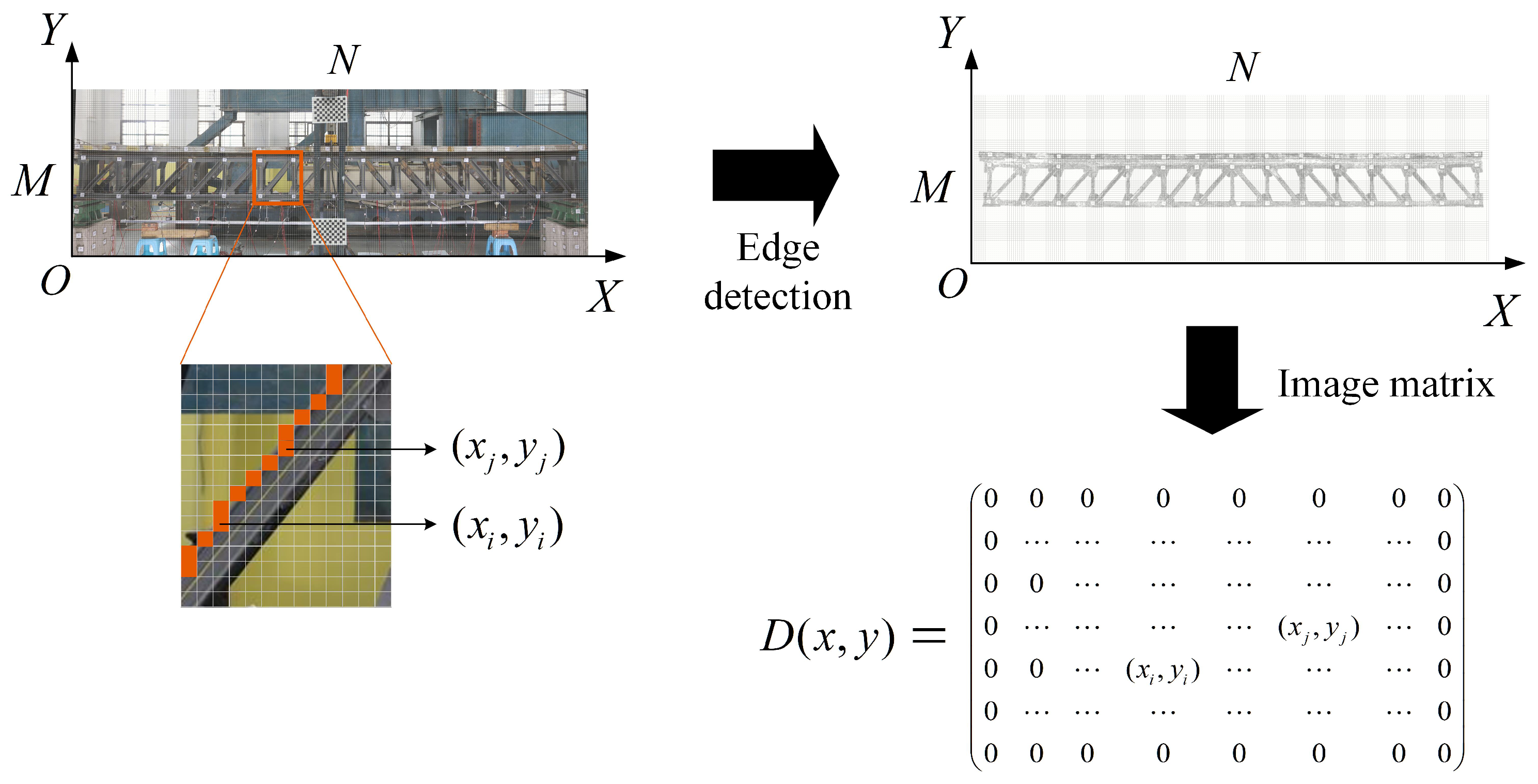
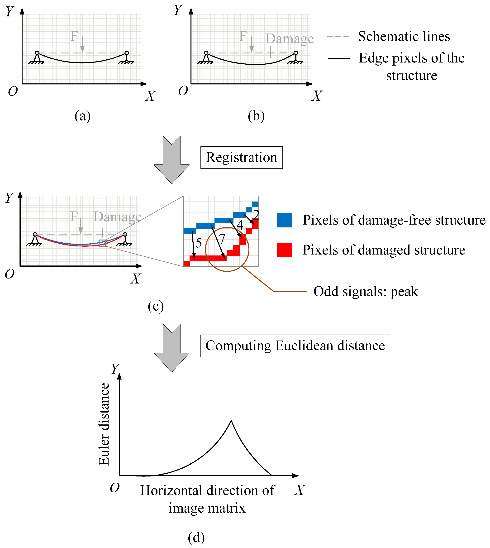
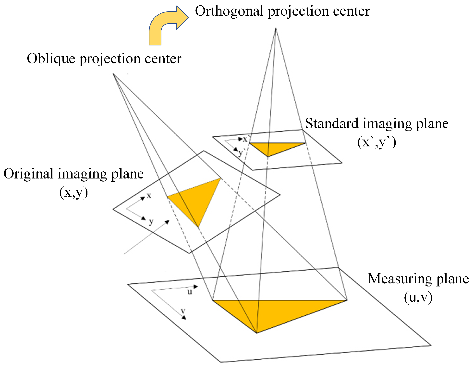
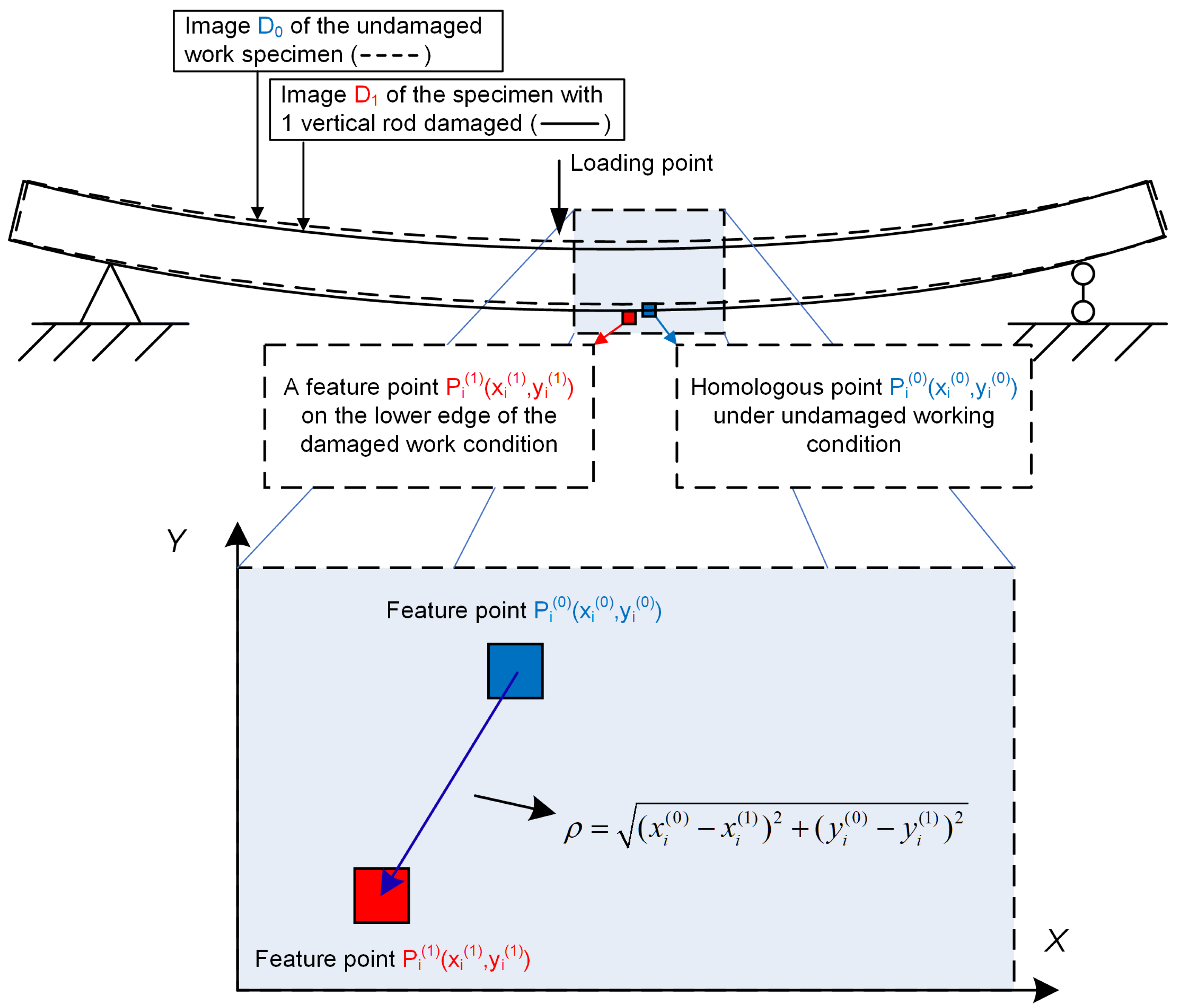
2.1. Damage Recognition Principle

The structure consists of several spatial units, and the characteristics of each unit can be reflected by the spatial stiffness matrix. Structural damage is essentially a change in the local stiffness of the structure: i.e., a change in the substructure stiffness matrix, and a change in the substructure position of the stiffness matrix, which can be interpreted as the appearance of bridge damage. The rod end force vector of an element can be expressed as

$$F^{\left(e\right)}={\left\{\begin{array}{cccccccccccc}{F}_{Ni}\hfill & F_{Qij}\hfill & F_{Qiz}\hfill & M_{ix}\hfill & M_{ij}\hfill & M_{iz}\hfill & F_{Nj}\hfill & F_{Qjy}\hfill & F_{Qjz}\hfill & M_{jx}\hfill & M_{jy}\hfill & M_{jz}\hfill \end{array}\right\}}^T$$

(1)

The rod end displacement vector of an element can be expressed as

$${\delta }^{\left(e\right)}={\left\{\begin{array}{cccccccccccc}{u}_i\hfill & v_i\hfill & w_i\hfill & {\theta }_{ix}\hfill & {\theta }_{iy}\hfill & {\theta }_i\hfill & u_j\hfill & v_j\hfill & w_j\hfill & {\theta }_{jx}\hfill & {\theta }_{jy}\hfill & {\theta }_{jz}\hfill \end{array}\right\}}^T$$

(2)

The stiffness equation of an element can be expressed as

$$F^{\left(e\right)}=K^{\left(e\right)}{\delta }^{\left(e\right)}$$

(3)

Several elements can be superimposed together to form a bridge stiffness matrix equation, as shown in Equation (4).

$$\left[\begin{array}{ccccccc}{k}_{11}& k_{12}& k_{13}& \cdots & k_{1,n-2}& k_{1,n-1}& k_{1,n}\\ k_{21}& k_{22}& k_{23}& \cdots & k_{2,n-2}& k_{2,n-1}& k_{2,n}\\ k_{31}& k_{32}& k_{33}& \cdots & k_{2,n-2}& k_{3,n-1}& k_{3,n}\\ ⋮& ⋮& ⋮& \ddots & ⋮& ⋮& ⋮\\ k_{n-2,1}& k_{n-2,2}& k_{n-2,3}& \cdots & k_{n-2,n-2}& k_{n-2,n-1}& k_{n-2,n}\\ k_{n-1,1}& k_{n-1,2}& k_{n-1,3}& \cdots & k_{n-1,n-2}& k_{n-1,n-1}& k_{n-1,n}\\ k_{n,1}& k_{n,2}& k_{n,3}& \cdots & k_{n,n-2}& k_{n,n-1}& k_{n,n}\end{array}\right]\left\{\begin{array}{c}{u}_1\\ v_1\\ w_1\\ ⋮\\ u_n\\ v_n\\ w_n\end{array}\right\}=\left\{\begin{array}{c}{X}_1\\ Y_1\\ Z_1\\ ⋮\\ X_n\\ Y_n\\ Z_n\end{array}\right\}$$

(4)

The bridge structural system necessarily follows the mechanical matrix equation as

$$\left\{d\right\}={\left[K\right]}^{-1}\left\{F\right\}$$

(5)

Equation (5) shows that there is an inevitable intrinsic connection between the displacement state $\left\{d\right\}$, which reflects the deformation characteristics of the bridge, and the stiffness matrix $\left[K\right]$, which characterizes the safety state of the bridge structure, and the various load effects $\left\{F\right\}$ acting on the bridge structure. If essential damage occurs in a part of the bridge structure, the stiffness of the corresponding member or linkage in the stiffness matrix $\left[K\right]$ is degraded, and there is a change in the displacement state $\left\{d\right\}$ of the bridge corresponding to it, meaning that the structural morphology will be different from the previous state. In summary, the changes in the morphology of a structure are bound to have a gradual development and evolution process due to the accumulation of internal damage and external loading effects, which is the landing point of various technologies in the field of structural health monitoring: trying to detect and capture the abnormal deformation of the structure as early as possible and then invert the safety state of the structure based on the monitoring data.

2.2. Image Matrix Similarity Damages Identification Method

The structural image matrix can be considered as a matrix consisting of pixel coordinates containing structural morphological information, denoted by the symbol a, as shown in Figure 1.

If a structure is damaged at a place, the degradation of its stiffness matrix will destroy the original deformation continuity, and the abnormal changes at the damage site will be more obvious compared with other parts, which will be characterized as discontinuous pixel distribution at the edge of the structure on the image, so the similarity test of the structure image matrix can be carried out for damage identification. Similarity analysis is an analytical method to evaluate the degree of similarity between two things, and the commonly used similarity analysis methods are the Euclidean metric, Pearson correlation coefficient, and cosine similarity [23]; in this paper, the Euclidean distance metric is used as the index of image matrix similarity analysis, and the similarity function can be expressed by Equation (6).

$$sim\left(D_0,D_1\right)=\rho \left(D_0\left(x^{\left(0\right)},y^{\left(0\right)}\right),D_1\left(x^{\left(1\right)},y^{\left(1\right)}\right)\right)=\sqrt{{\left(x^{\left(0\right)}-x^{\left(1\right)}\right)}^2+{\left(y^{\left(0\right)}-y^{\left(1\right)}\right)}^2}$$

(6)

where $sim\left(D_0,D_1\right)$ is the similarity between two image matrices $D_0$ and $D_1$.

$\rho \left(D_0\left(x^0,y^0\right),D_1\left(x^1,y^1\right)\right)$ represent the Euclidean distance between the corresponding elements of the two image matrices $D_0$ and $D_1$. $x^0$, $y^0$, $x^1$, and $y^1$, respectively, represent the horizontal and vertical coordinates of the elements in $D_0$ and $D_1$. From the relationship between structural damage and morphology mentioned earlier, it can be seen that when the structure is not damaged, the similarity distribution of the structure under different working conditions is a straight line or a continuous smooth curve. After the damage occurs, the matrix similarity curve will show an abnormal peak response at the damage site, and the principle is shown in Figure 2.

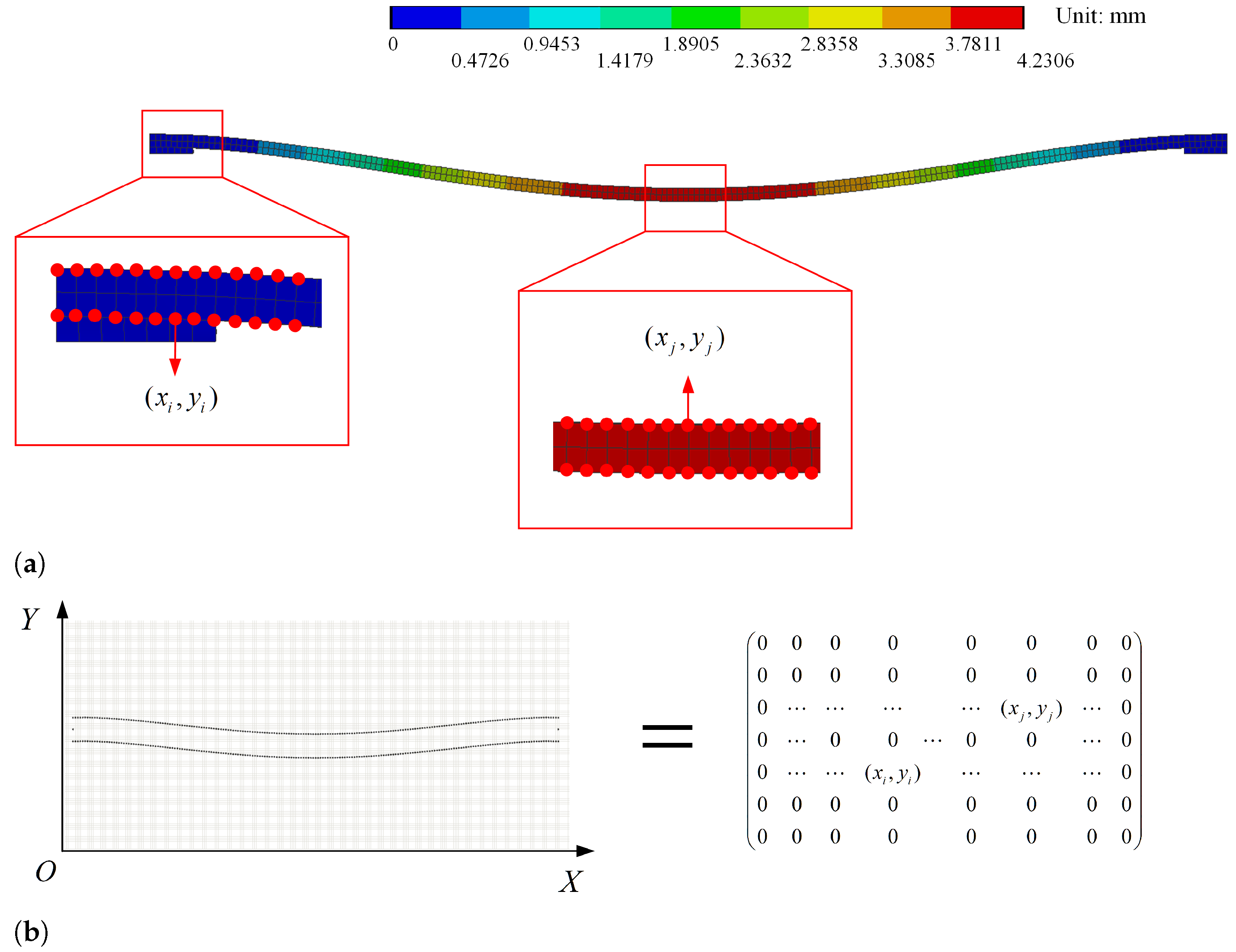
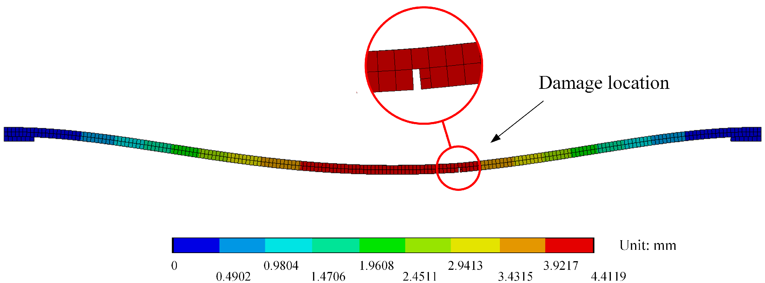
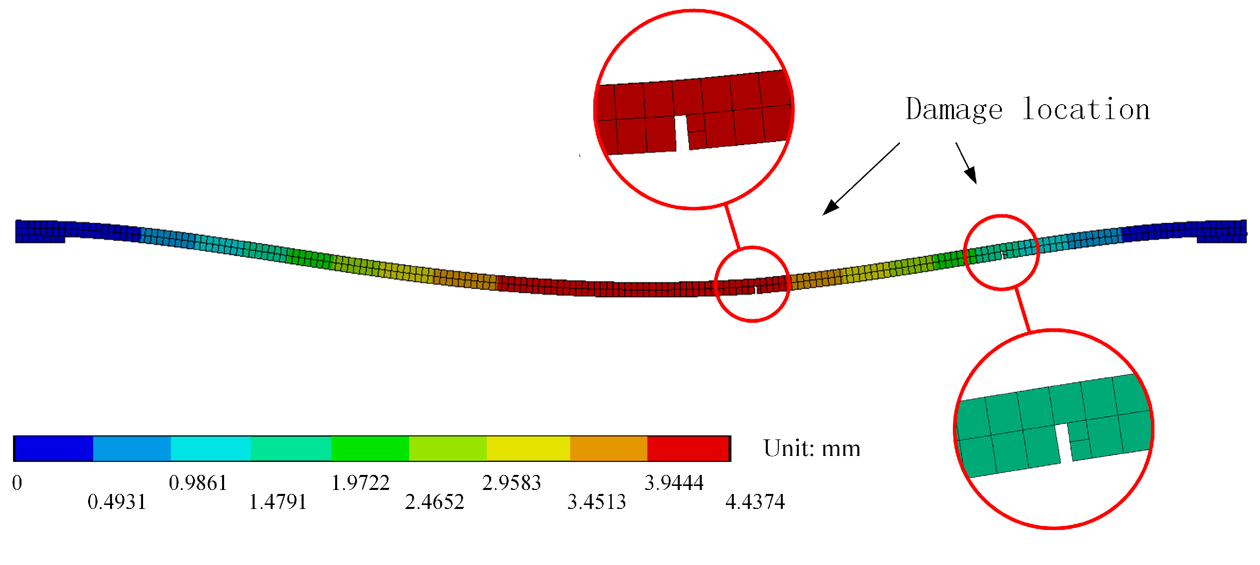
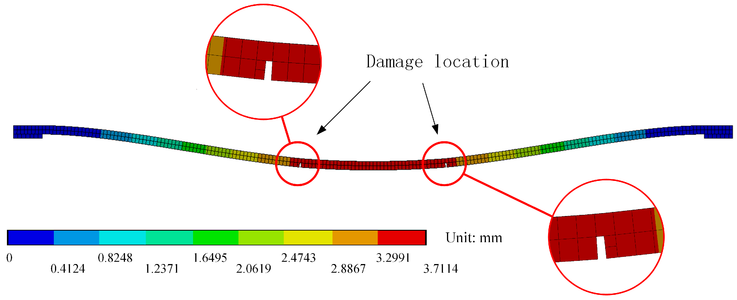
2.3. Numerical Validation of Image Matrix Similarity Damage Localization Method

A numerical model of the simply supported beam is established to verify the above damage localization method. The model span is 500 mm, and the cross-section is a rectangular section of size 20 mm × 6 mm. The beam is of uniform mass, the material is structural steel, the modulus of elasticity is 2 × ${10}^5$ MPa, and the concentrated force of 1 kN acts in the middle of the span, as shown in Figure 3.

The mesh nodes on the $X-Z$ surface of the numerical model are simulated as image matrices. The deflection diagram and the corresponding image matrix of the undamaged model under the action of 1 kN concentrated force are shown in Figure 4.

(1) Single damage identification verification.

A damage crack is set at 200 mm from the right support with a width of 1 mm and a depth of 3 mm. Figure 5 shows the deflection of the damage model.

The Euclidean distances of the corresponding points of the structure with no damage and post-damage are calculated separately under the same load. Figure 6 shows the Euclidean distances of the upper and lower edges of the model.

The image matrix similarity curves in Figure 6 have obvious peaks at the damage locations, indicating that the image matrix similarity analysis method can effectively identify the location of structural damage in the single damage condition.

(2) Eccentric multi-damage identification verification.

Set two cracks 100 mm and 200 mm from the right support, with a crack width of 1 mm and depth of 3 mm. The multi-damage model deformation is shown in Figure 7.

Calculate the Euclidean distances of the homologous point in the image matrix of undamaged and post-damaged structures. The results of the analysis of the upper and lower edges of the simply supported beam are shown in Figure 8.

(3) Symmetric multi-damage identification verification.

Similarly, set up two cracks 200 mm from each side of the support with a width of 1 mm and a depth of 3 mm. The symmetric multi-damage model is shown in Figure 9.

The Euclidean distances of the homologous points in the image matrix of the undamaged and post-damaged structures are calculated. The results of the upper and lower edge analysis are shown in Figure 10.

According to the above analysis, it is found that the extreme points of the similarity curve may not be the damage locations, and the discontinuity points are the damage locations, which is consistent with the deformation coordination of the structure. Therefore, the second-order derivative of the Euclidean distance curve is used to amplify this damage signal, so the similarity is calculated by Equation (7).

$$sim\left(D_0,D_1\right)=\left|\frac{d^2\rho }{d{x}^2}\right|$$

(7)

The image matrix similarity analysis of the finite element model for single-damage and multi-damage conditions is re-performed using Equation (7), and the results can be obtained as in Figure 11.

Figure 11 illustrates that the results of image matrix similarity analysis under multi-damage conditions are similar to those of single-damage identification, and the image matrix similarity has a clear peak at the damage location. In summary, the image matrix similarity analysis method can accurately locate the damage location on a multi-damaged simply supported beam. It is verified that the difference in the location of the damage does not affect its regularity.

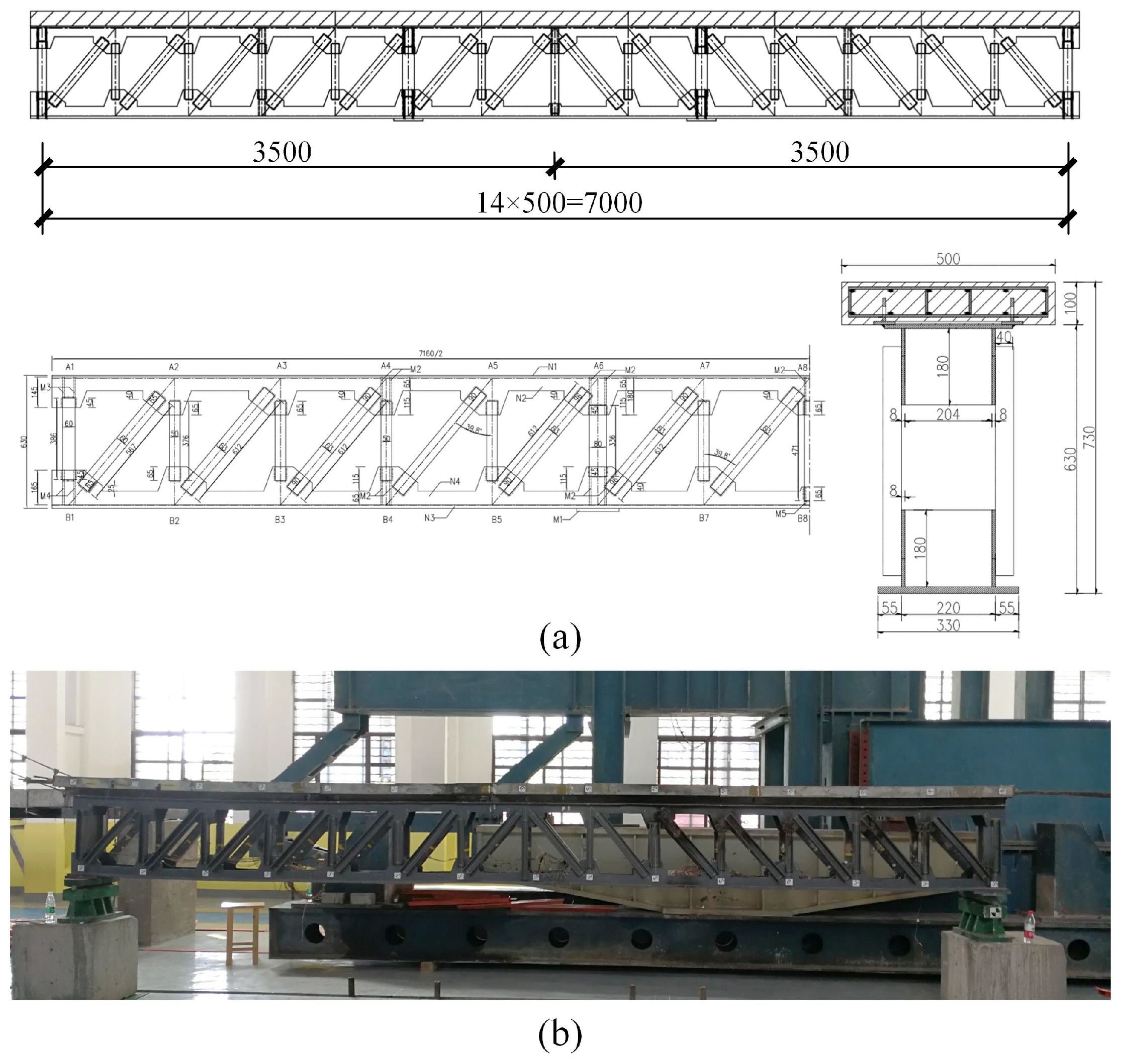
3. Static Test of a Steel Truss–Concrete Composite Beam

To test the effectiveness of the image matrix similarity method proposed in this paper for damage identification on real structures, steel truss–concrete composite beam specimens have been designed and fabricated. The image matrix was obtained by extracting the pixel coordinates of the structure edges in the photos. The displacements extracted from the images were compared with the data from the dial gauges and the 3D laser scanner to ensure the accuracy of the images in describing the structural deformation.

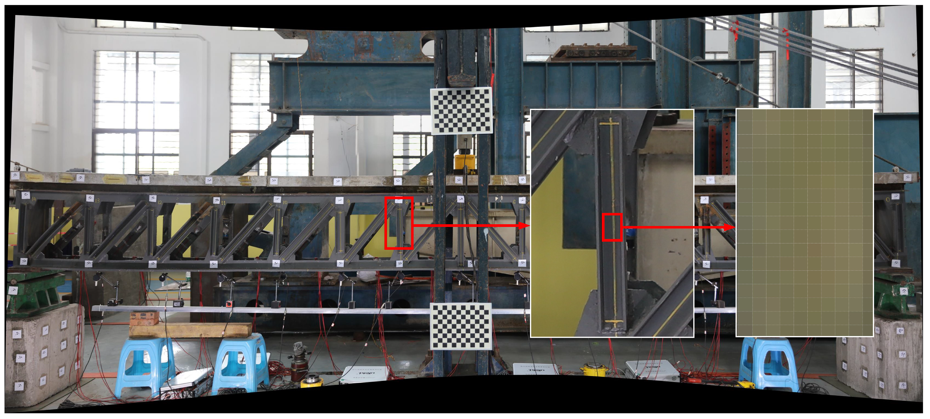
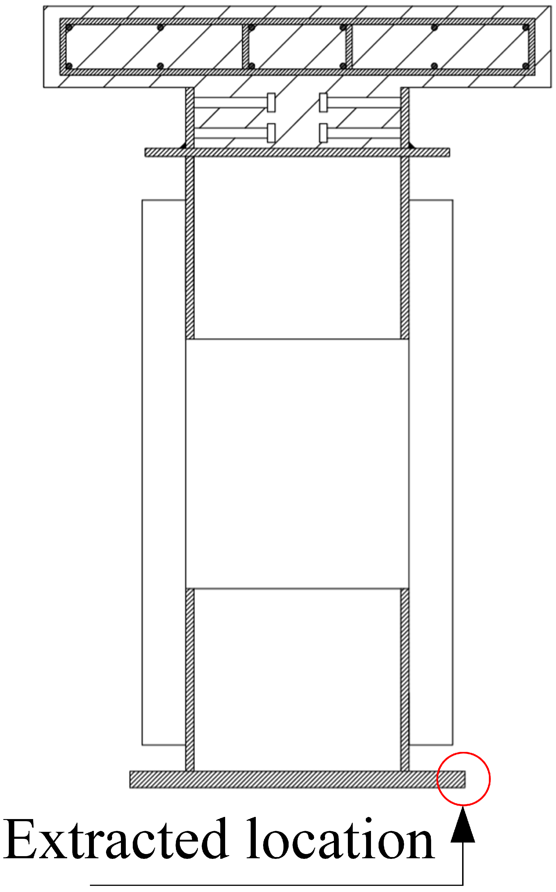
3.1. Specimen Preparation

Figure 12a gives the dimensions and construction of the steel truss–concrete composite beam for the test. The bridge deck slab is made of C50 precast concrete with T-shaped cross section, total height of 140 mm, width of 500 mm and flange plate thickness of 100 mm. The bridge deck slab is assembled from 5 standard sections and 2 end sections, the length of the middle 5 standard sections is 1000 mm and the length of the end 2 sections is 1080 mm. The steel trusses are fabricated and welded in the factory. The completed steel truss–concrete composite beam specimen is shown in Figure 12b.

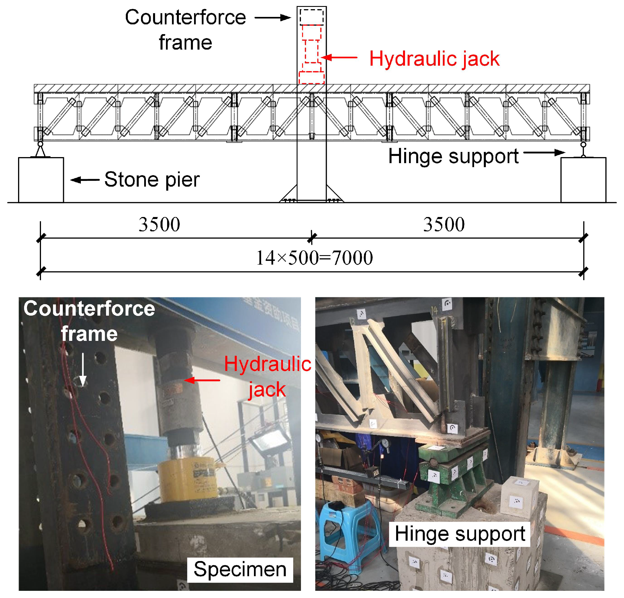
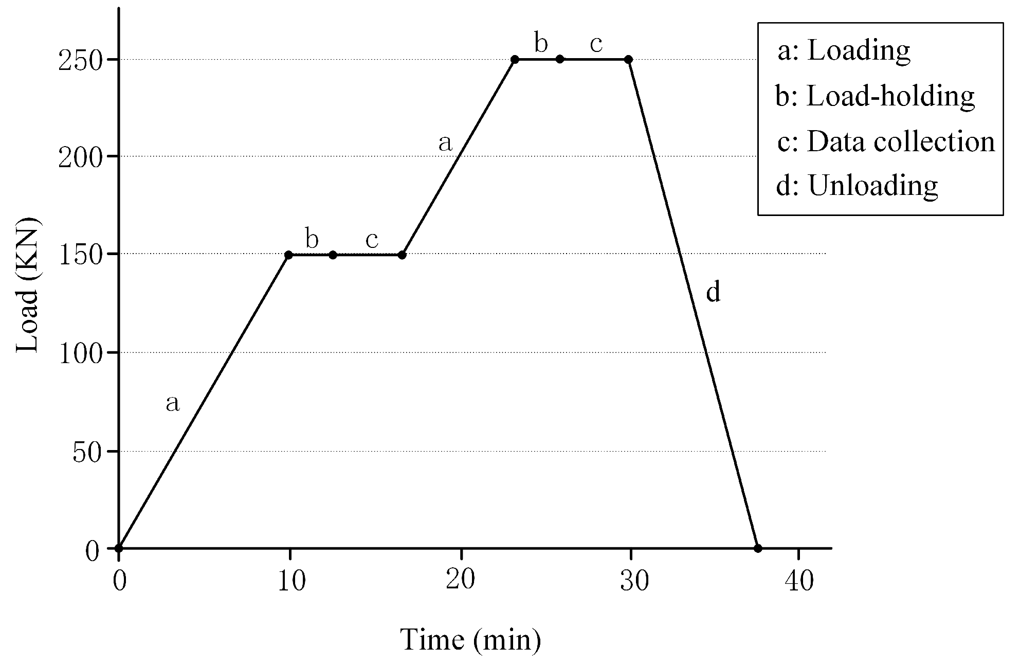
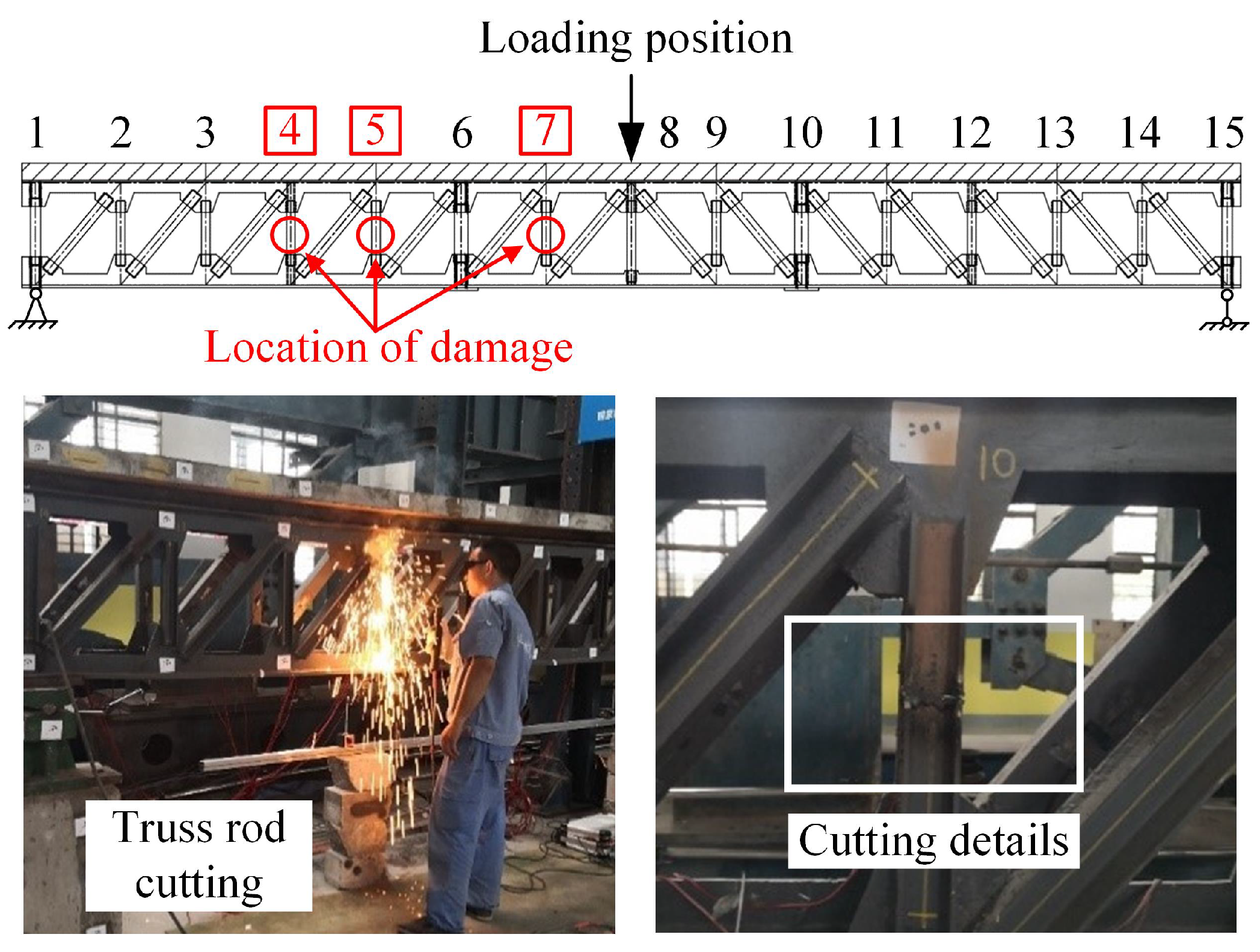
3.2. Test Loading Protype and Damage

The loading point of the test beam is located in the middle of the span. Hydraulic jack (Maximum load 50 tons) and counterforce frame are used as loading devices, as shown in Figure 13, and pressure sensors are installed on the jack to ensure accurate loading. The specimen support type is the hinged support. The test beams in each damage condition were loaded with 150 kN and 250 kN as load class. After each class of loading, hold the load for two minutes to ensure the full deformation of the test beam, and then take pictures of the specimen and collect the displacement data. The loading protype is shown in Figure 14.

The damage to the rod was simulated by cutting the truss vertical rod, and the damage working condition of the specimen is shown in

Table 1. Summary of damage and load conditions.

Damage Conditions	Location of Damage	Loading Situation	Load (KN)
No damage		${\mathrm{O}}_1$	0
		${\mathrm{O}}_2$	150
		${\mathrm{O}}_3$	250
Damage to a rod	Rod No. 7	${\mathrm{A}}_1$	0
		${\mathrm{A}}_1$	150
		${\mathrm{A}}_1$	250
Damage to two rods	Rod No. 5	${\mathrm{B}}_1$	0
		${\mathrm{B}}_1$	150
		${\mathrm{B}}_1$	250
Damage to three rods	Rod No. 4	${\mathrm{C}}_1$	0
		${\mathrm{C}}_1$	150
		${\mathrm{C}}_1$	250

. The vertical rod number and the location of the damaged vertical rod are shown in Figure 15.

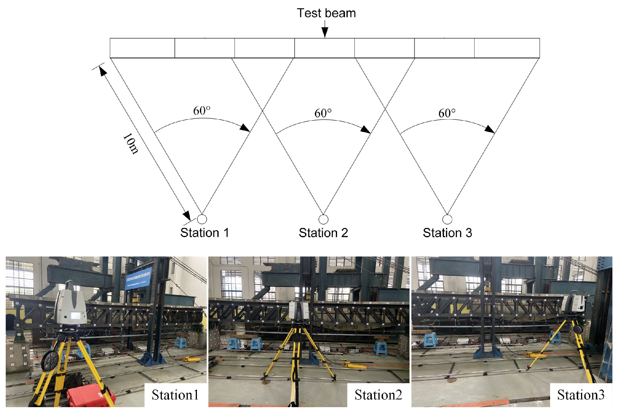
3.3. Image Data Acquisition

Using Canon 5DSR camera to take photos of the experiment specimen, the camera and lens parameters are shown in

Table 2. Camera and lens parameters.

Number of Pixels	Sensor Size	Image Size	Aspect Ratio	Pixel Size	Lens Models	Lens Relative Aperture	Focal Length
50.6 million	$36\times 24\mathrm{mm}$	$8688\times 5792$	3:2	4.14 µm	EF 24–70 mm f/2.8LII	F2.8–F22	24–70 mm

, and the camera calibration [24] results are shown in

Table 3. Calibration results.

Actual Image Size (Pixel)		Actual Image Centre Size (Pixel)		Actual Focal Length (mm)		Radial Distortion Parameters			Tangential Distortion Parameters
X	Y	$x_0$	$y_0$	$f_x$	$f_y$	$k_1$	$k_2$	$k_3$	$p_1$	$p_2$
8688	5792	4319.74	2885.85	24.3	24.3	0.122	0.108	0.024	0	0

. The directly acquired specimen images are affected by the natural perspective and show obvious near-large and far-small features (Figure 16), resulting in the images not correctly reflecting the deformation of the structure, so a perspective transformation of the specimen images is required.

Image geometric transformation refers to the geometric transformation of image pixel positions without changing the original image content, mainly including translation, rotation, scaling, reflection, and misalignment. The perspective transformation is a combination of basic geometric transformations. The image of the measured structure will be distorted, when photographed under the condition of non-orthogonal projection [25,26]. If the image is mapped to the plane where the target structure is measured, called the measuring plane, in other words, the camera shoots perpendicular to the measurement plane, the real shape of the target structure can be obtained, and the perspective transformation model is shown in Figure 17.

Using the projection center of the camera as the origin to establish a three-dimensional Cartesian coordinate system, called the camera 3D coordinate system, let the original imaging plane be the $xy$ plane, with the focal point at ${[0,0,f]}^T$, ($f>0$). A two-dimensional coordinate system is established in the measuring plane, and the origin of this coordinate system is ${\left[x_0,y_0,z_0\right]}^T$ in the camera 3D coordinate system, the unit vector in the X-axis direction is ${\left[u_1,u_2,u_3\right]}^T$, and the unit vector in the Y-axis direction is ${\left[v_1,v_2,v_3\right]}^T$. The vectors adhere to the rules as follows:

$$\left\{\begin{array}{c}{u}_1{v}_1+u_2{v}_2+u_3{v}_3=0\\ u_1^2+u_2^2+u_3^2=v_1^2+v_2^2+v_3^2=1\end{array}\right.$$

(8)

Then, the point with coordinates ${[u,v]}^T$ in the target object plane (measuring plane) can be expressed in the camera 3D coordinate system as

$$u\left[\begin{array}{c}{u}_1\\ u_2\\ u_3\end{array}\right]+v\left[\begin{array}{c}{v}_1\\ v_2\\ v_3\end{array}\right]+\left[\begin{array}{c}{x}_0\\ y_0\\ z_0\end{array}\right]$$

(9)

Assuming that the point in the imaging plane has point coordinates ${[x,y,0]}^T$, then $\exists k\in R$ must satisfy the following equation.

$$u\left[\begin{array}{c}{u}_1\hfill \\ u_2\hfill \\ u_3\hfill \end{array}\right]+v\left[\begin{array}{c}{v}_1\hfill \\ v_2\hfill \\ v_3\hfill \end{array}\right]+\left[\begin{array}{c}{x}_0\hfill \\ y_0\hfill \\ z_0\hfill \end{array}\right]-\left[\begin{array}{c}0\hfill \\ 0\hfill \\ f\hfill \end{array}\right]=k\left(\left[\begin{array}{c}0\hfill \\ 0\hfill \\ f\hfill \end{array}\right]-\left[\begin{array}{c}x\hfill \\ y\hfill \\ 0\hfill \end{array}\right]\right)$$

(10)

The following equations can be obtained.

$$-k\left[\begin{array}{c}x\hfill \\ y\hfill \end{array}\right]=u\left[\begin{array}{c}{u}_1\hfill \\ u_2\hfill \end{array}\right]+v\left[\begin{array}{c}{v}_1\hfill \\ v_2\hfill \end{array}\right]+\left[\begin{array}{c}{x}_0\hfill \\ y_0\hfill \end{array}\right]=\left[\begin{array}{ccc}{u}_1\hfill & v_1\hfill & x_0\hfill \\ u_2\hfill & v_2\hfill & y_0\hfill \end{array}\right]\left[\begin{array}{c}u\hfill \\ v\hfill \\ 1\hfill \end{array}\right]$$

(11)

$$kf=u{u}_3+v{v}_3+z_0-f=\left[\begin{array}{ccc}{u}_3\hfill & v_3\hfill & z_0-f\hfill \end{array}\right]\left[\begin{array}{c}u\hfill \\ v\hfill \\ 1\hfill \end{array}\right]$$

(12)

From Equation (12), we then obtain the following:

$$-k=\left[\begin{array}{ccc}-\frac{u_3}{f}\hfill & -\frac{v_3}{f}\hfill & -\frac{z_0-f}{f}\hfill \end{array}\right]\left[\begin{array}{c}u\hfill \\ v\hfill \\ 1\hfill \end{array}\right]$$

(13)

Combining this with Equation (11) gives

$$-k\left[\begin{array}{c}x\hfill \\ y\hfill \\ 1\hfill \end{array}\right]=\left[\begin{array}{ccc}{u}_1& v_1& x_0\\ u_2& v_2& y_0\\ -\frac{u_3}{f}& -\frac{v_3}{f}& -\frac{z_0-f}{f}\end{array}\right]\left[\begin{array}{c}u\hfill \\ v\hfill \\ 1\hfill \end{array}\right]$$

(14)

Introducing the parameter matrix M, we obtain

$$M=\left[\begin{array}{ccc}{u}_1& v_1& x_0\\ u_2& v_2& y_0\\ -\frac{u_3}{f}& -\frac{v_3}{f}& -\frac{z_0-f}{f}\end{array}\right]$$

(15)

If the measuring plane does not pass through the focal point ${[0,0,f]}^T$, then the matrix M must be an invertible matrix. Under normal operation, the focal point does not lie on the measuring plane, so the matrix M is always an invertible matrix. When the camera moves to a new position to photograph the target structure, the relative spatial position of the camera and the target structure changes. The change can be equated to the condition whereby the camera imaging plane does not move, while the focal length and the actual spatial position of the target structure change accordingly. Let the coordinates of the camera focus become ${\left[0,0,f^{\prime }\right]}^T$ and the origin of the measuring plane become ${\left[x_0^{\prime },y_0^{\prime },z_0^{\prime }\right]}^{\mathrm{T}}$. The unit vectors in the x, y axis of the scenic plane become ${\left[u_1^{\prime },u_2^{\prime },u_3^{\prime }\right]}^{\mathrm{T}}$ and ${\left[v_1^{\prime },v_2^{\prime },v_3^{\prime }\right]}^{\mathrm{T}}$, respectively. Similarly, $\exists k^{\prime }\in R$ makes the coordinate point ${[u,v]}^{\mathrm{T}}$ on the measuring plane and the point ${\left[x^{\prime },y^{\prime },0\right]}^{\mathrm{T}}$ of the imaging plane corresponding to the point ${[u,v]}^{\mathrm{T}}$ satisfy the following equation.

$$-k^{\prime }\left[\begin{array}{c}{x}^{\prime }\\ y^{\prime }\\ 1\end{array}\right]=\left[\begin{array}{ccc}{u}_1^{\prime }& v_1^{\prime }& x_0^{\prime }\\ u_2^{\prime }& v_2^{\prime }& y_0^{\prime }\\ -\frac{u_3^{\prime }}{f^{\prime }}& -\frac{v_3^{\prime }}{f^{\prime }}& -\frac{z_0^{\prime }-f^{\prime }}{f^{\prime }}\end{array}\right]\left[\begin{array}{c}u\hfill \\ v\hfill \\ 1\hfill \end{array}\right]$$

(16)

Then, the parameter matrix $M^{\prime }$ is shown as

$$M^{\prime }=\left[\begin{array}{ccc}{u}_1^{\prime }& v_1^{\prime }& x_0^{\prime }\\ u_2^{\prime }& v_2^{\prime }& y_0^{\prime }\\ -\frac{u_3^{\prime }}{f^{\prime }}& -\frac{v_3^{\prime }}{f^{\prime }}& -\frac{z_0^{\prime }-f^{\prime }}{f^{\prime }}\end{array}\right]$$

(17)

Combining Equations (14) and (16) yields

$$-k^{\prime }\left[\begin{array}{c}{x}^{\prime }\hfill \\ y^{\prime }\hfill \\ 1\hfill \end{array}\right]=M^{\prime }\left[\begin{array}{c}u\hfill \\ v\hfill \\ 1\hfill \end{array}\right]=-k{M}^{\prime }{M}^{-1}\left[\begin{array}{c}x\hfill \\ y\hfill \\ 1\hfill \end{array}\right]$$

(18)

Assuming

$$M^{\prime }·M^{-1}=\left[\begin{array}{ccc}{m}_{11}\hfill & m_{12}\hfill & m_{13}\hfill \\ m_{21}\hfill & m_{22}\hfill & m_{23}\hfill \\ m_{31}\hfill & m_{32}\hfill & m_{33}\hfill \end{array}\right]$$

(19)

Then, we can obtain

$$\left\{\begin{array}{c}{k}^{\prime }{x}^{\prime }=k\left(m_{11}x+m_{12}y+m_{13}\right)\\ k^{\prime }{y}^{\prime }=k\left(m_{21}x+m_{22}y+m_{23}\right)\\ k^{\prime }=k\left(m_{31}x+m_{32}y+m_{33}\right)\end{array}\right.$$

(20)

Therefore, there is

$$\left\{\begin{array}{c}{x}^{\prime }=\frac{m_{11}x+m_{12}y+m_{13}}{m_{31}x+m_{32}y+m_{33}}\hfill \\ y^{\prime }=\frac{m_{21}x+m_{22}y+m_{23}}{m_{31}x+m_{32}y+m_{33}}\hfill \end{array}\right.$$

(21)

The point $(x,y)$ on the original imaging plane can be transformed into the new imaging point $\left(x^{\prime },y^{\prime }\right)$ by perspective transformation, and $\left(x^{\prime },y^{\prime }\right)$ is the point of the orthorectified image that is not affected by perspective. The orthographic projection of the test beam after perspective transformation is shown in Figure 18.

As can be seen from Figure 18, the specimen image after perspective transformation is no longer influenced by perspective and is free from the imaging characteristic of “large near and small far”. Thus, the specimen image has the characteristics of orthographic projection, and the deformation information of the structure can be analyzed on this basis.

3.4. Accuracy-Verified Data Acquisition

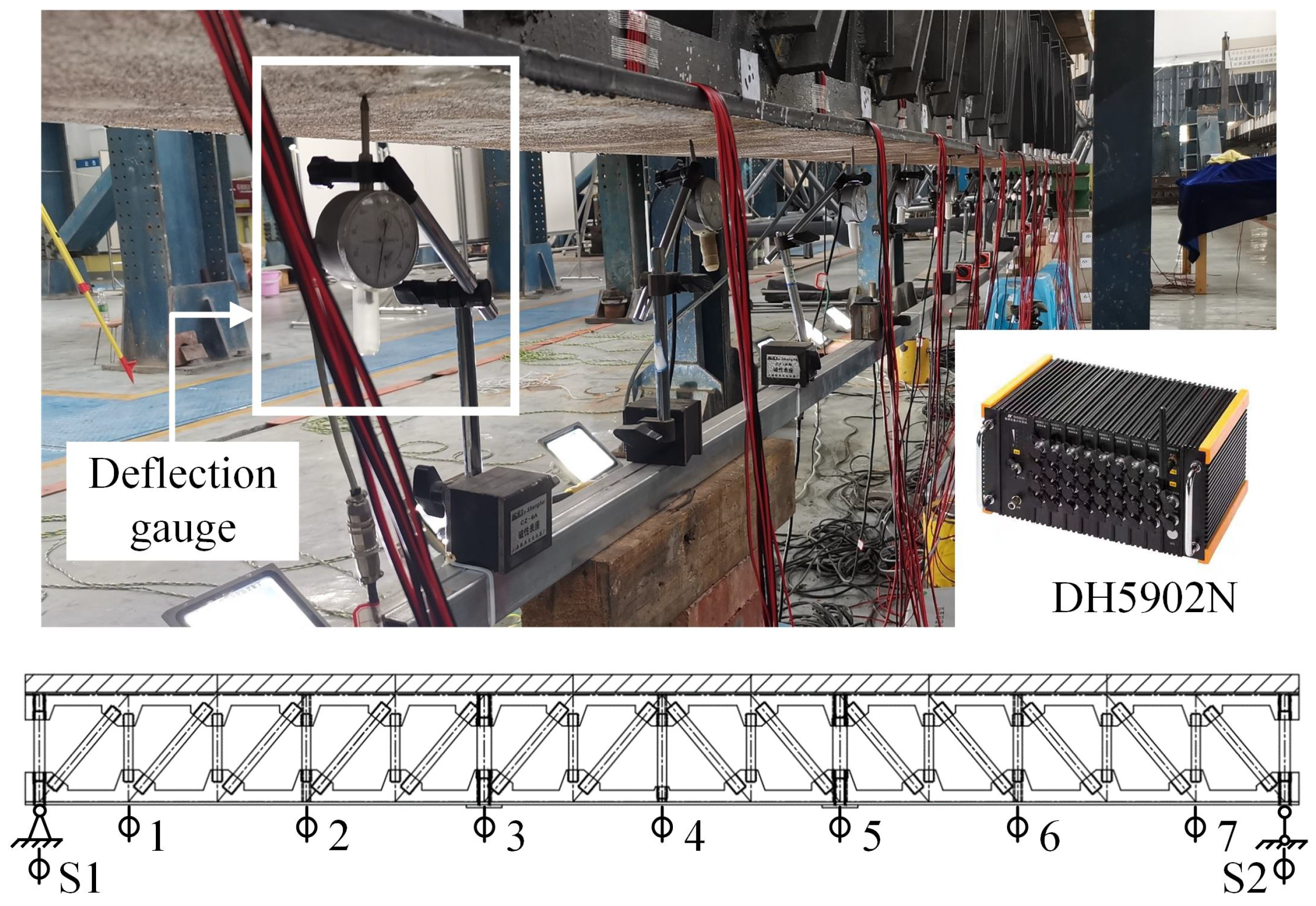
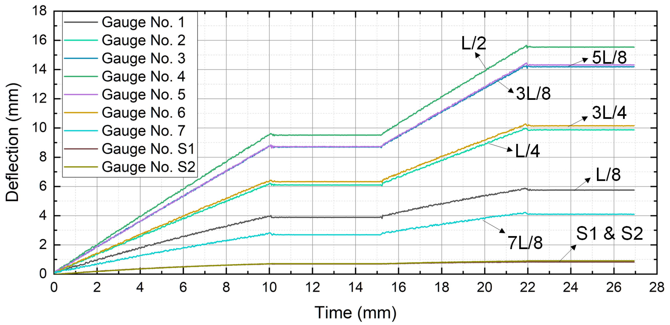
3.4.1. Deflection Gauge Measurement

The deflection gauge is a traditional deformation measurement instrument that is often used as a basis for verifying the accuracy of experimental data because of its high accuracy [27].The conventional displacement measurement method of this test uses the deflection electric measurement system, which includes deflection gauge (range 0–30 mm, accuracy 0.01–mm) and DH5902N test and analysis system. The DH5902 acquisition frequency is set to 1 time in 2 seconds. Seven deflection gauges are installed directly below the vertical rod of the test beam at $L/8$, $L/4$, $3L/8$, $L/2$, $5L/8$, $3L/4$ and at the two supports, and the data acquisition system is arranged as shown in Figure 19.

The deflections of different load classes for each damage condition measured by the deflection gauge are summarized in

Table 4. Deflection measurement results.

Number of Damaged Rods	Working Conditions	Load (kN)	Deflection Gauge Values (mm)
			S1	L/8	L/4	3L/8	L/2	5L/8	3L/4	7L/8	S2
0	${\mathrm{O}}_1$	0	0	0	0	0	0	0	0	0	0
	${\mathrm{O}}_2$	150	0.717	3.884	6.101	8.696	9.514	8.725	6.33	2.696	0.732
	${\mathrm{O}}_3$	250	0.844	5.751	9.875	14.194	15.539	14.32	10.15	4.101	0.913
1	${\mathrm{A}}_1$	0	0	0	0	0	0	0	0	0	0
	${\mathrm{A}}_2$	150	0.689	2.401	5.949	8.541	10.693	8.921	6.198	2.001	0.694
	${\mathrm{A}}_3$	250	0.828	4.213	9.668	13.871	16.815	14.103	10.104	3.319	0.851
2	${\mathrm{B}}_1$	0	0	0	0	0	0	0	0	0	0
	${\mathrm{B}}_2$	150	0.704	3.356	5.959	8.764	10.61	8.923	6.358	2.603	0.688
	${\mathrm{B}}_3$	250	0.813	5.336	9.62	14.107	16.67	14.521	10.14	4.288	0.843
3	${\mathrm{C}}_1$	0	0	0	0	0	0	0	0	0	0
	${\mathrm{C}}_2$	150	0.655	4.155	6.479	9.246	10.583	9.524	6.384	3.139	0.664
	${\mathrm{C}}_3$	250	0.805	6.102	10.234	14.589	16.631	14.782	10.134	4.558	0.822

. The process of collecting deflection data under no-damage conditions is shown in Figure 20.

From Table 4, it is found that in some positions, the damaged bars increase but the deflections decrease. The reason is that the steel joist–concrete combination beam has a complex internal support bar system, and the difference of structural deflection before and after the damage is not significant, which indicates that the deflection is not sensitive to the damage of the complex structure. Conventional single-point measurement damage identification methods are not ideal for this type of structure. Compared with the conventional damage identification methods, using this type of specimen as the test object can fully demonstrate the innovation and efficiency of structural holographic morphological data in the damage identification problem.

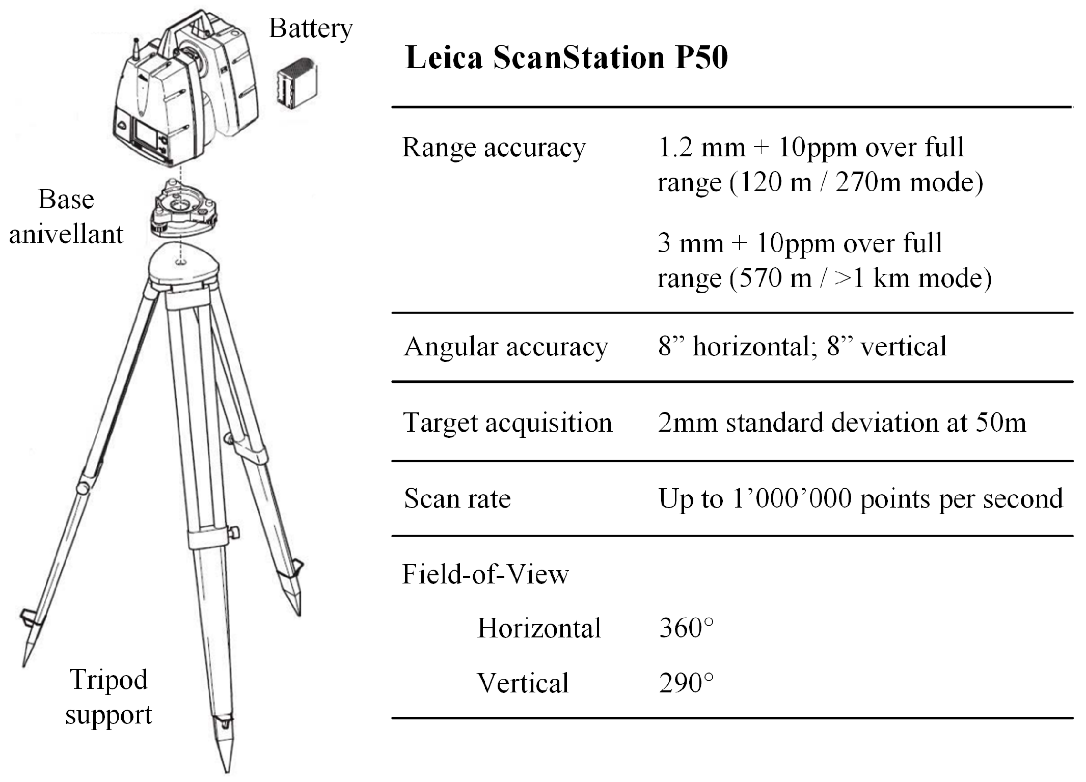
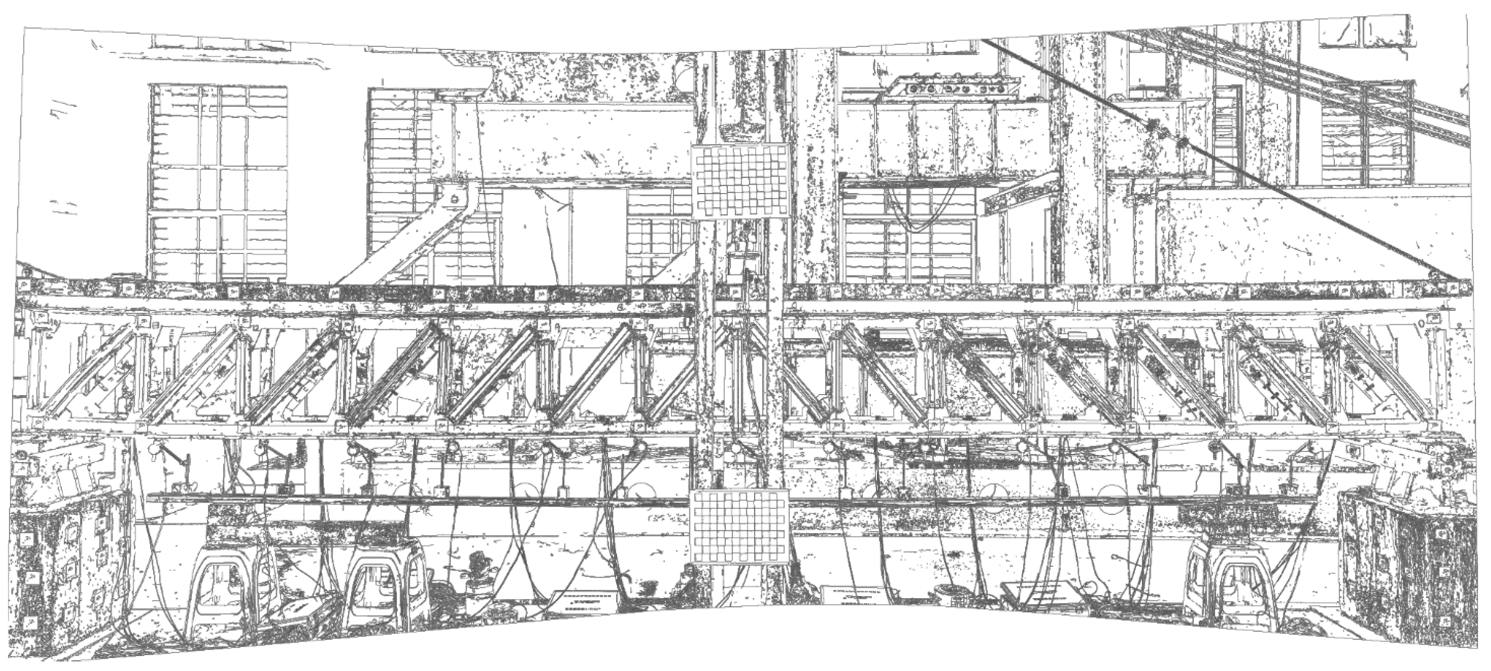
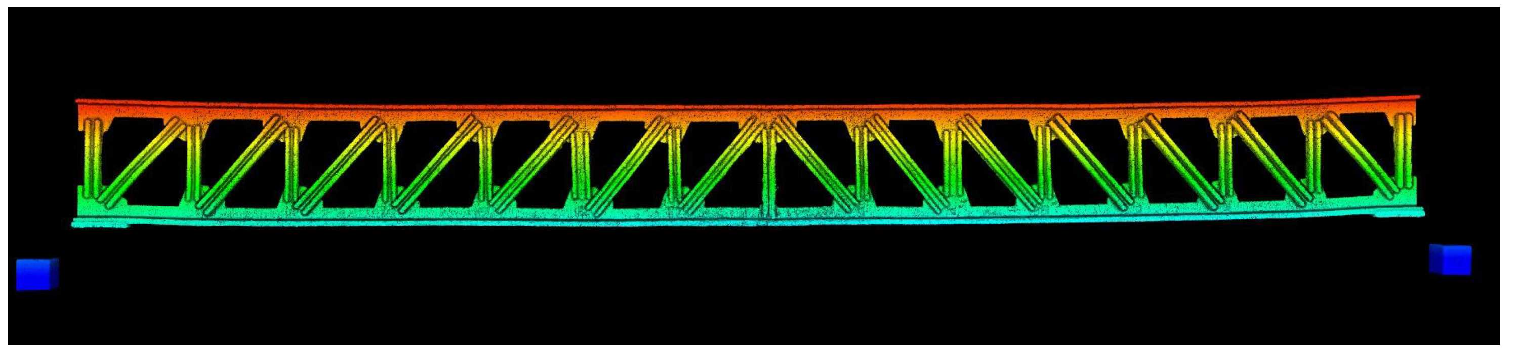
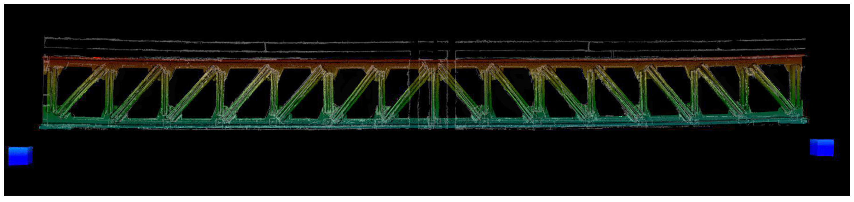
3.4.2. Three-Dimensional Laser Point Cloud Data Acquisition

Three-dimensional laser scanning technology is a non-contact, fast, and accurate measurement technique, and its application to the inspection of engineering structures has become a new trend of development [28,29]. It is widely used in the field of accurate deformation monitoring for bridges, buildings, tunnels, pipe racks, and other projects [30]. Ling Xiaochun [31] studied the influence of distance, incident angle, and target color on the accuracy of the scanner during measurement. Using the plane fitting method to analyze the accuracy, it was verified that the accuracy of a ground-based 3D laser is 1 to 2 mm, which meets the nominal accuracy; the angle measurement accuracy is about ${15}^{\prime \prime }$; and the point position accuracy can reach the millimeter level. Moreover, this technology is based on the principle of laser ranging and can acquire a large amount of morphological data of the target object, so it is feasible to use 3D laser scanning data for the comparison and verification of images.

The Leica ScanStation P50 3D laser scanner is used to verify the extracted structural holographic deformation data, the basic parameters of which are shown in Figure 21. The scanning resolution is 0.8 mm/10 m, the point accuracy is 30 mm/50 m, the target acquisition accuracy is 2 mm/50 m, and the noise accuracy is 0.4 mm/10 m. According to the analysis results of the scanning angle effect on the point cloud density obtained from the previous study [32], the following scanning measurement verification test scheme was used: the scanning pattern was three-station joint scanning, the scanning radius was set to 10 m, and the scanning angle was $\left[-{30}^{\circ },{30}^{\circ }\right]$. The layout of the site is shown in Figure 22.

Under this scanning scheme, the theoretical value of high-density point cloud coverage on the side of the test beam is >91.5% with high accuracy, which makes the 3D laser scanning data valuable for verifying the morphological deviations extracted from the images. The verification process of 3D laser scanning on the holographic morphology of the structural images is detailed in Section 4.3. In order to match the 3D laser scanning accuracy verification test, 20 mm diameter coded marker points were arranged on the upper and lower chord node plates of the test beam, and the location and number of the marker points are shown in Figure 23. The results of the 3D laser scan are shown in Figure 24.

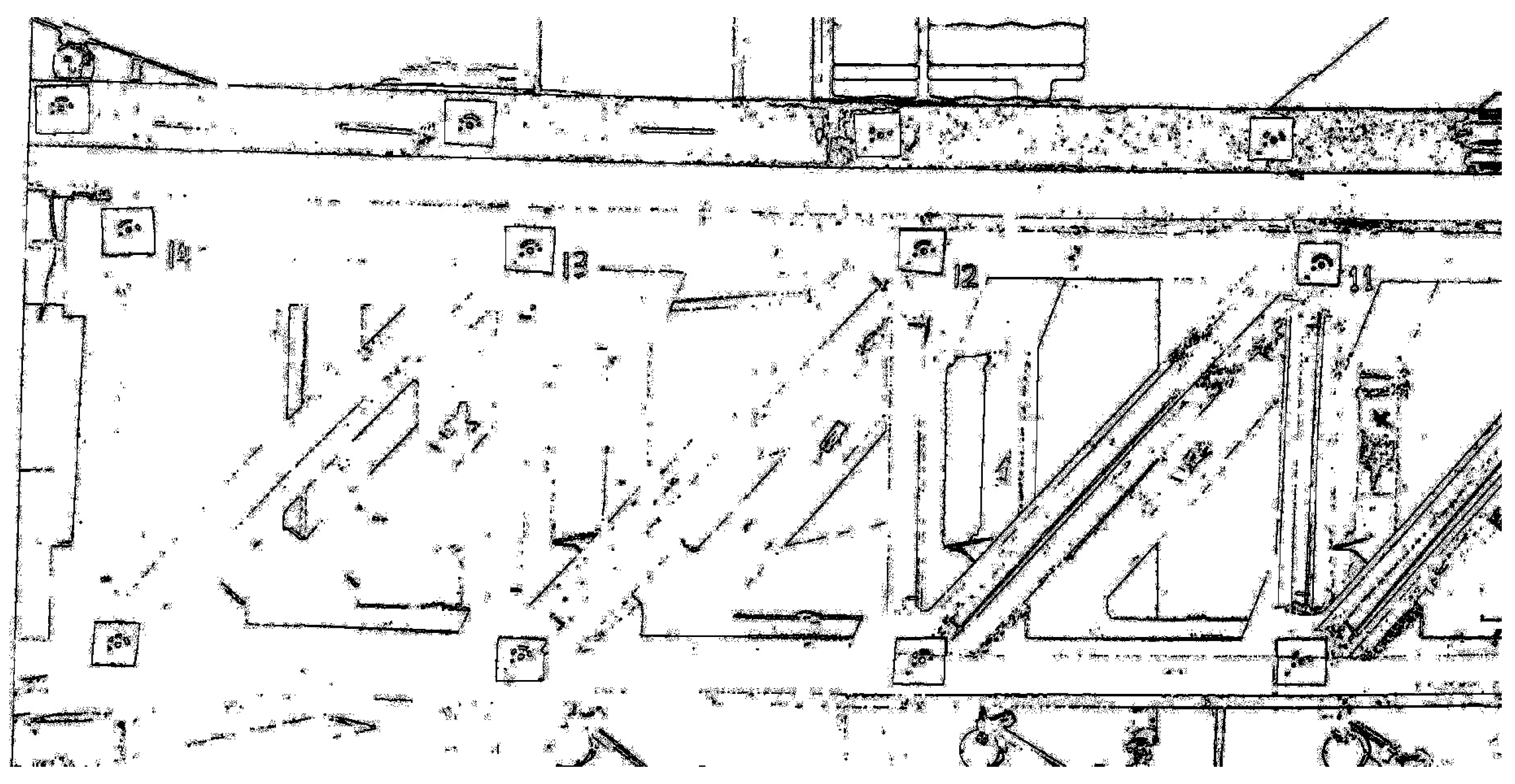
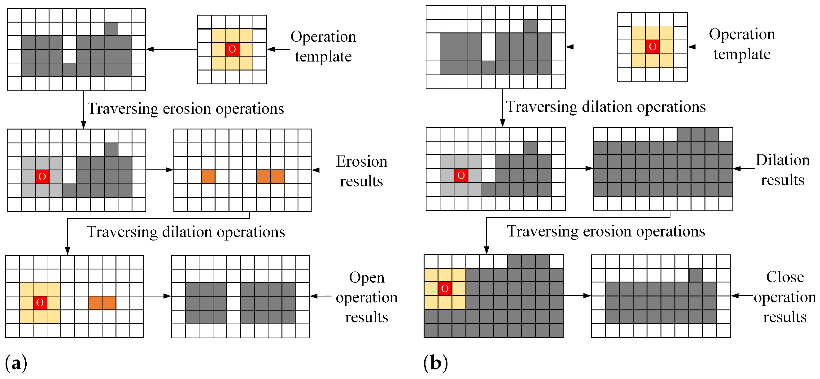
4. Bridge Structure Morphology Extraction

Based on the equivalent orthographic projection image, the features of the test beam under the ${\mathrm{O}}_1$ working condition obtained by using the SIFT feature point extraction method [33] are shown in Figure 25.

The main body edge contains the morphological information of the structure, which is the main area of structural feature point distribution and constitutes an important carrier of structural holographic deformation data. After simplifying the feature extraction results of the ${\mathrm{O}}_1$ working condition, unnecessary environmental feature points are removed, and the main features of the structure are highlighted as shown in Figure 26.

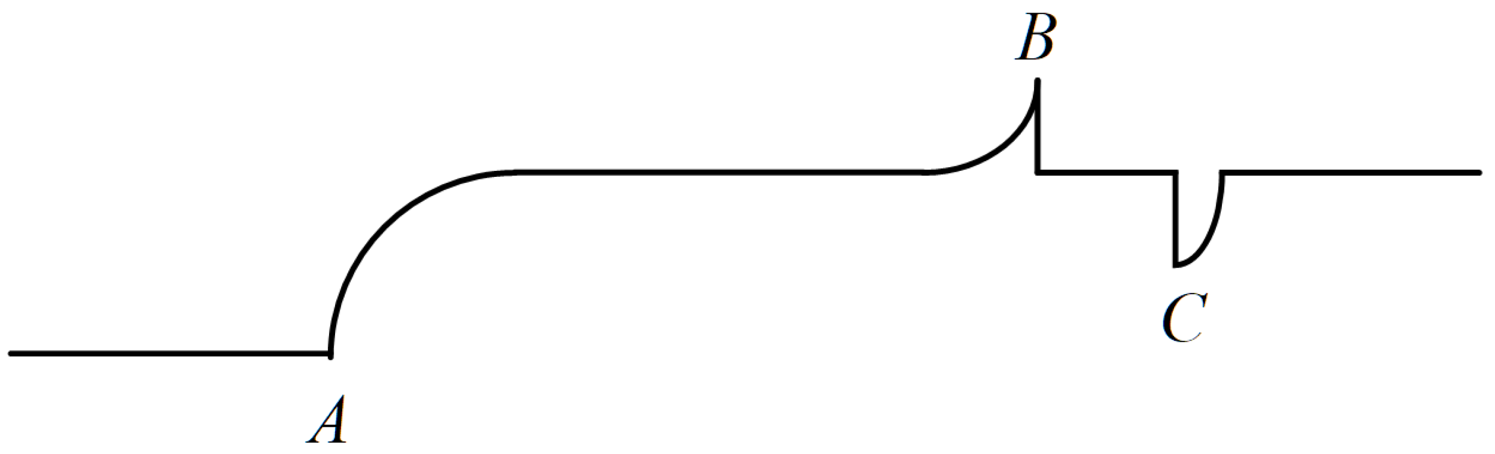
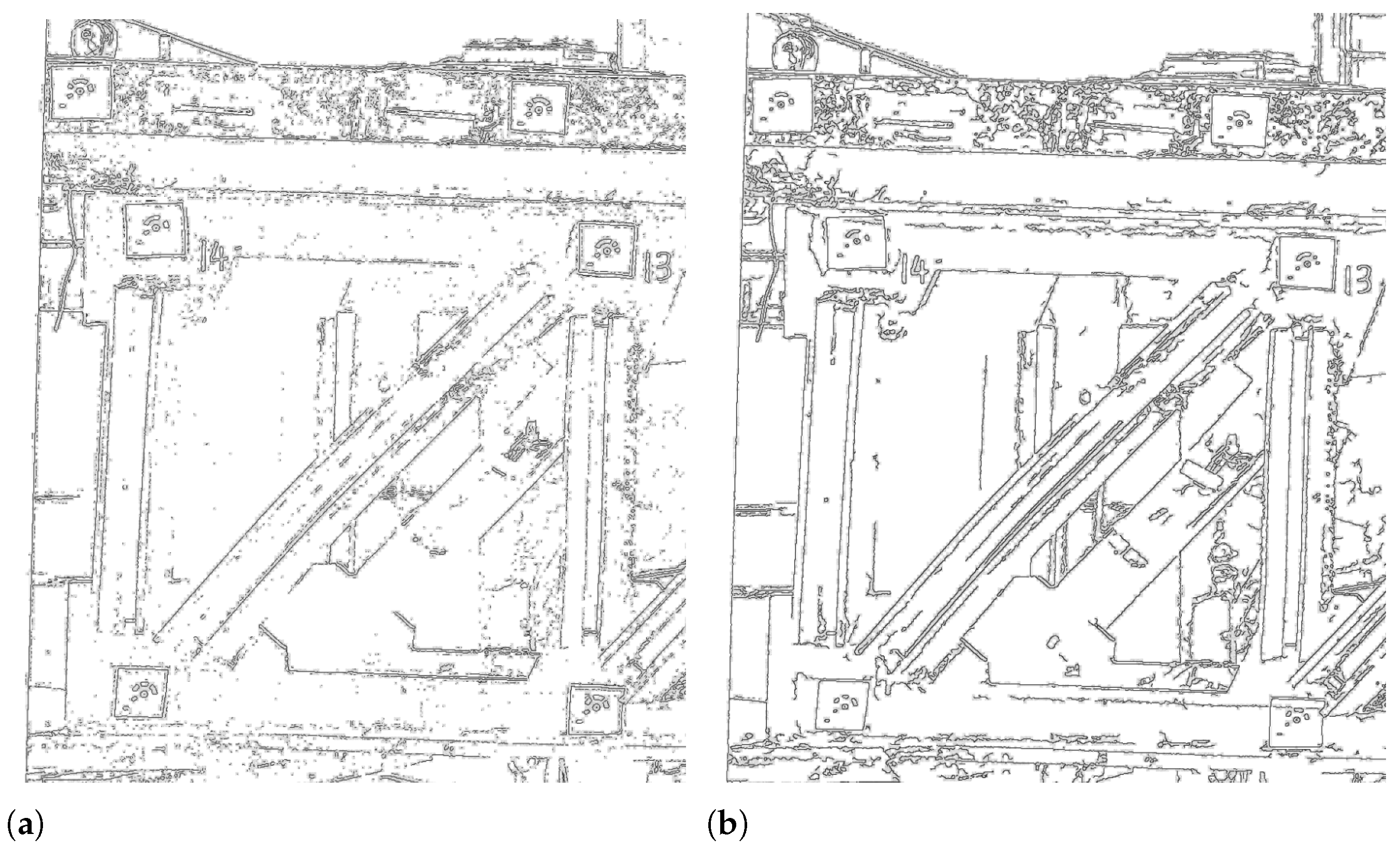
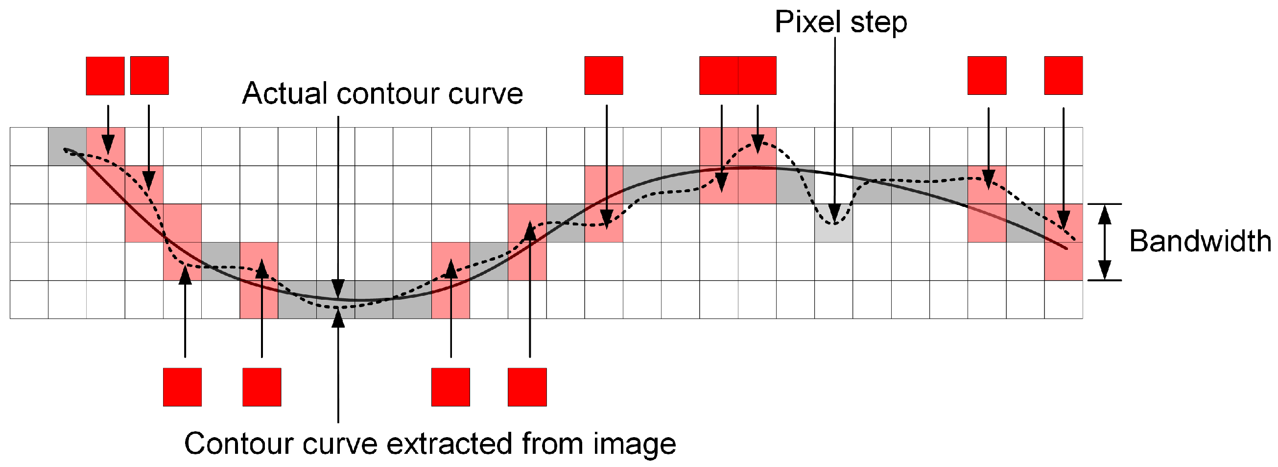
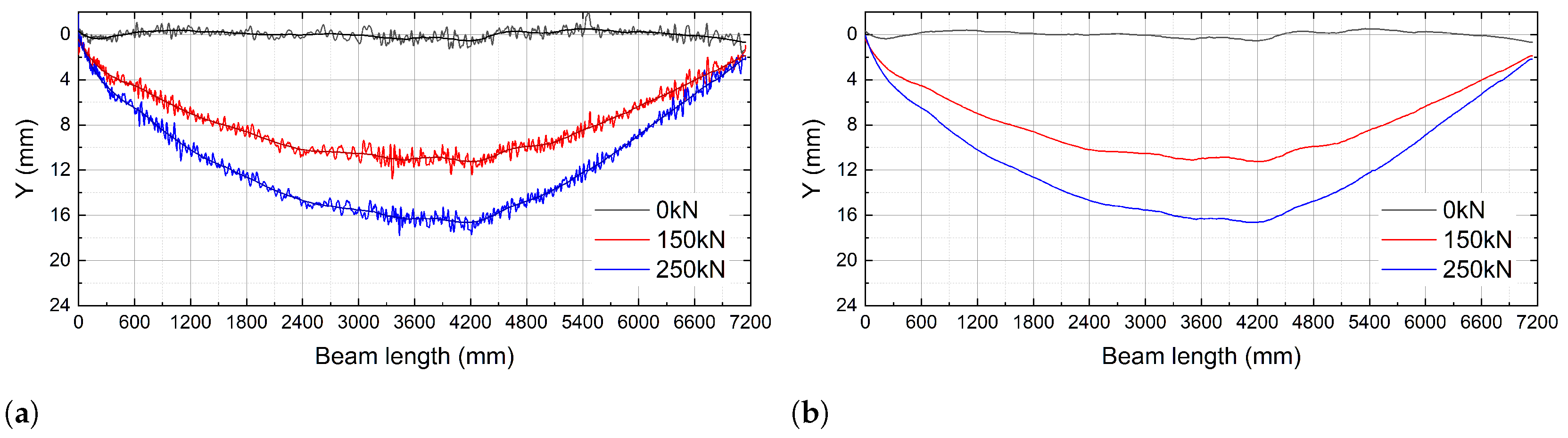
4.1. Regression of Discontinuous Edges of Test Beam Images

The intrinsic nature of image features is points with discontinuous grayscale variations, and the dramatic grayscale variations imply the presence of high-frequency components of the signal of interest in the vicinity of the features. The previously extracted structural image features are not enough for structural holographic deformation monitoring. The reason for this is that it is difficult to clearly delineate the high-frequency components of the signal of interest on the bridge structure images from the environmental noise. For example, in a segment of the bridge edge image signal shown in Figure 27, point A is the ideal signal identified in the feature extraction process, and there is a step in the feature gray change at this point. Since the differential operation in the feature extraction process leads to the amplification of the noise signal, whether the step signal identified at points B and C is the true edge of the structure needs to be treated with caution. In fact, points B and C are most likely the synthesis of the characteristic signal with some noise.

Due to the variable environment of bridge structure monitoring, points with natural grayscale excess and continuous gradient changes, such as point A in Figure 27, are rarer on actual bridge images. The geographical and lighting environment in which the bridge is located would make most of the structural features accompanied by environmental noise, forming a large number of feature points with complex components, such as B and C. This leads to the real feature signal being smoothed out by the Gaussian spatial filter after the noise is mixed with the structural feature signal, and the actual performance of this problem on the bridge image is edge discontinuity and missing edge information (as shown in Figure 28). Structural edges are an important source of feature point generation, the missing edges cannot provide stable and rich point source data for structural holographic morphology analysis, and the missing edges need to be regressed.

The dilation and erosion operations are the two most important image boundary processing methods in morphology [34,35,36,37,38], and they are also the key means to achieve the concentration of structure-extracted edges toward the actual edges and the regression of edge breakpoints in this section. We use $f(x,y)$ to describe grayscale images, $b(i,j)$ for structural elements, and $D_f$, and $D_b$ to define the domains of f and b. The dilation and erosion operations are described in Equations (22) and (23).

(1) Definition of erosion:

$$(f\Theta b)(x,y)=min\left\{f(x+i,y+i)-b(i,j)\mid (x+i,y+j)\in D_f;(i,j)\in D_b\right\}$$

(22)

(2) Definition of dilation:

$$(f\oplus b)(x,y)=max\left\{f(x-i,y-i)-b(i,j)\mid (x-i,y-j)\in D_f;(i,j)\in D_b\right\}$$

(23)

The edges of the images obtained by the erosion or dilation operations alone are rough, and the edge noise composition is complicated in the actual image processing, so it is necessary to combine the erosion and dilation operations. In order to eliminate the external discrete points of the structure edge and smooth the structure edge, the process of first erosion and then dilation is used for edge treatment. For the problem of discontinuous breaks in the edge, the process of first dilation and then erosion is used to naturally connect the edge breaks while ensuring that the edge distribution does not expand outward. The morphological process of first erosion and then dilation is called the open operation (Equation (24)), and the process of first dilation and then erosion is called the closed operation (Equation (25)), and the above basic morphological operations are shown schematically in Figure 29.

(3) Open operation definition.

$$f(x,y)\circ b(x,y)=\left[\right(f\Theta b)\oplus b](x,y)$$

(24)

(4) Closed operation definition.

$$f(x,y)•b(x,y)=\left[\right(f\oplus b)\Theta b](x,y)$$

(25)

From Figure 29, it can be seen that morphological operations can improve the continuity of edges and achieve the approximation of discontinuous edges to continuous edges when there are discontinuities in the edges of bridge images. The before-and-after comparison of the regression of the discontinuous edge of the test beam image is shown in Figure 30. It can be seen that after edge regression, the discrete edge points of the image become continuous curves, while smoothing out most of the noise. This image can be initially used to quantitatively identify the target deformation.

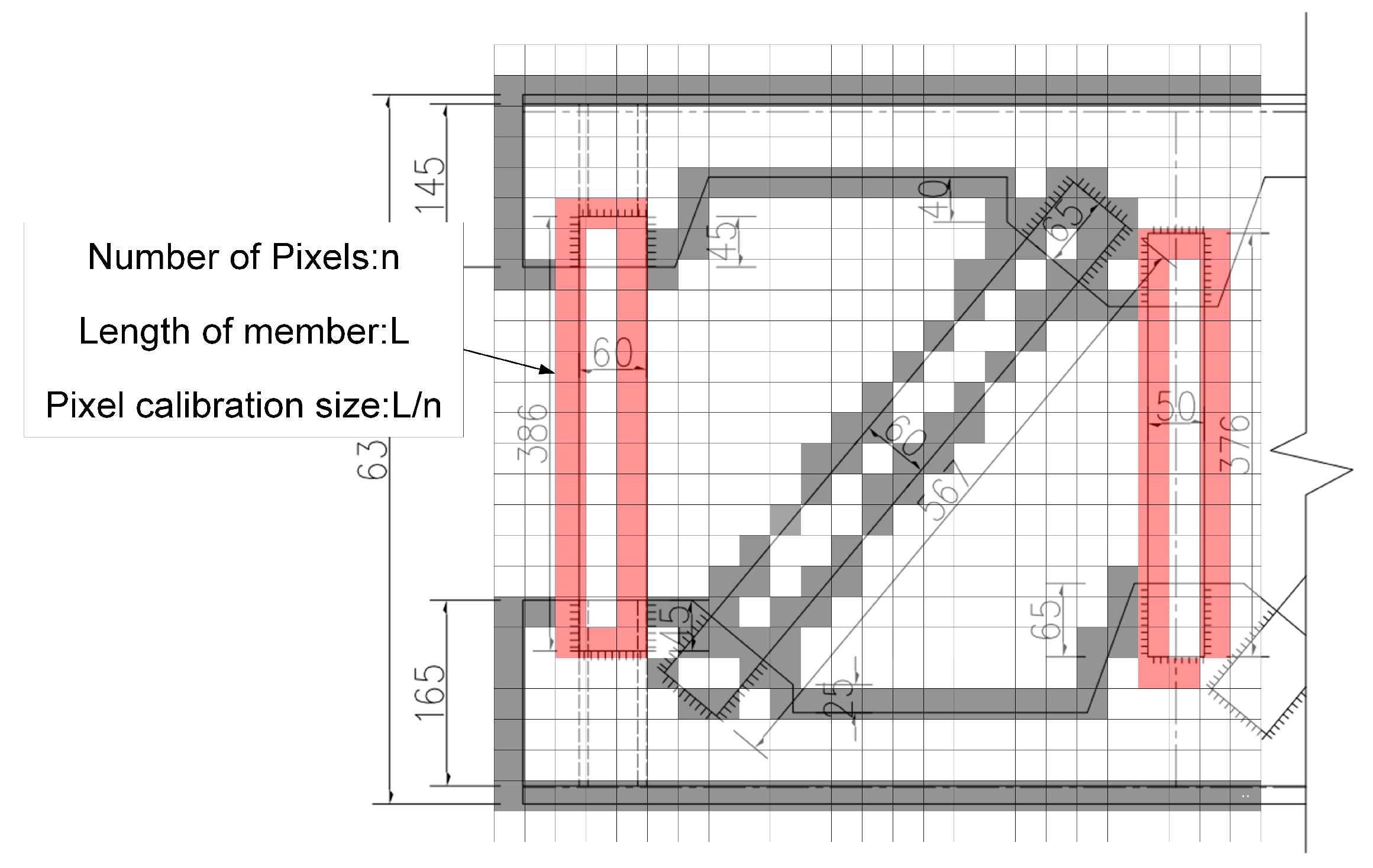
4.2. Calibration of Bridge Image Resolution

The deformation of the structure is reflected in the image as a change in the pixel position of the deformed area. In the same shooting environment, how much deformation can cause the pixel position to change becomes a resolution issue for bridge image deformation monitoring. Theoretically, the deformation value has to be larger than the pixel size to be recognized by the bridge structure deformation monitoring method. The yellow calibration line is drawn in the truss vertical rod (Figure 31), which is a series of regular pixel matrix arrangements on the image, the physical size of these pixels in relation to the actual specimen is the monitoring resolution, and the calibration model is shown in Figure 32. The resolution calibration is calculated as $R=L/n$ (mm/pixel). The test beam has a total of 15 vertical rods, and yellow calibration lines are drawn in the middle of each vertical rod during the test. The exact length of each calibration line is actually measured, the number of pixels of the calibration line is counted on the image, and then the monitoring resolution is obtained as shown in

Table 5. Resolution calibration table.

Vertical Truss Rod Number	Number of pixels	Calibration Line Length (mm)	Calibrated Value (mm/px)	Calibration Average (mm/px)
1	1986	367.17	0.1849	0.1771
2	1999	359.21	0.1797
3	1993	360.1	0.1807
4	1991	357.3	0.1795
5	1998	356.32	0.1783
6	1994	312.39	0.1567
7	1989	355.91	0.1789
8	2654	453.94	0.171
9	1982	356.83	0.18
10	1993	321.44	0.1613
11	1988	357.77	0.18
12	1987	356.75	0.1795
13	1994	361.37	0.1812
14	1989	363.1	0.1826
15	1983	359.47	0.1813

.

The monitoring resolution of the bridge image is obtained by calibrating the pixel size. Using this resolution, the pixel dimensions of bridge images can be converted to deformation monitoring dimensions, and then the measured deformation value of the structure can be obtained from the pixel bit difference.

4.3. Structure Body Morphology Extraction Results Validation

In this section, the morphology of the main body of the structural image extracted in Section 3.4.2 is verified quantitatively using 3D laser scanning measurements that have the ability to describe the holographic morphology of the structure and proven experience in engineering application.

After the 3D point cloud of the test beam is eliminated from perspective, a digital orthophoto map (DOM) of the point cloud of the test beam is made as shown in Figure 33. The calibrated morphology of the test beam obtained in Section 4.2 is superimposed on Figure 33, and the comparison of the main morphology of the structural image and the actual morphology of the DOM is shown in Figure 34.

As can be seen from Figure 34, the main morphology of the extracted structure image matches well with the actual morphology of the structure obtained by 3D machine light scanning. The quantitative verification of the structural morphology extracted from the images follows the method used in the previous study [32]: the point cloud data are constituted as the NURBS surface of the test beam, the coordinates of the top left and bottom left vertices of the vertical rods are extracted, and all the vertical rod heights $L_i$ and vertical rod spacing $D_i$ of the test beam are calculated according to the patterns of Figure 35; at the same time, $L_i^{\prime }$ and $D_i^{\prime }$ of the same positions of the vertical rods in the structural morphology of the images are calculated, and the comparison results are shown in

Table 6. Test beam image vertical bar height $L_i^{\prime }$, spacing $D_i^{\prime }$ extraction result verification table.

Vertical Rod Number	Rod Height Extracted from 3D Scan ${\mathit{L}}_{\mathit{i}}$/mm	Rod Height Extracted from Image ${\mathit{L}}_{\mathit{i}}^{\prime }$/mm	Spacing Extracted from 3D Scan ${\mathit{D}}_{\mathit{i}}$/mm	Spacing Extracted from Image ${\mathit{D}}_{\mathit{i}}^{\prime }$/mm
1	387.96	387.31
		(−0.65)	509.87	509.43
2	379.41	380.24		(−0.44)
		(0.83)	503.01	503.74
3	380.67	380.31		(0.73)
		(−0.36)	501.74	502.21
4	377.67	378.06		(0.47)
		(0.39)	500.58	499.76
5	376.83	376.26		(−0.82)
		(−0.57)	491.36	491.05
6	332.09	332.59		(−0.31)
		(0.5)	517.49	517.79
7	375.21	375.59		(0.30)
		(0.38)	503.05	503.22
8	473.48	474.46		(0.17)
		(0.98)	507.04	507.28
9	376.98	376.76		(0.24)
		(−0.22)	523.49	524.12
10	341.28	342.06		(0.63)
		(0.78)	488.16	488.74
11	377.17	377.25		(0.58)
		(0.08)	508.43	507.96
12	376.15	375.74		(−0.47)
		(−0.41)	509.25	509.44
13	381.90	382.41		(0.19)
		(0.51)	509.56	509.86
14	383.17	383.45		(0.30)
		(0.28)	513.39	512.81
15	379.50	379.21		(−0.58)
		(−0.29)

The values in parentheses are the absolute errors of the image morphology extraction values of the vertical rods compared with the 3D laser scanning results.

.

From Table 6, the length and spacing of vertical rods in the image-extracted structural morphology are consistent with the actual morphology of the structure with a maximum absolute error of 0.98 mm, indicating that the extracted image morphology of the test beam can correctly reflect the actual morphology of the structure. Therefore, the holographic morphological changes of any characteristic position of the structure in the image can be quantitatively analyzed.

5. Damage Identification based on Image Matrix Similarity

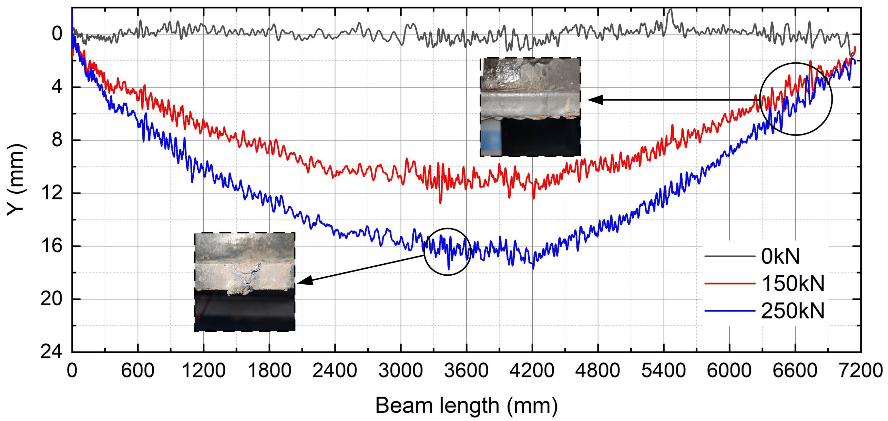
5.1. Bridge Structure Edge Deformation Analysis

Since the deflection gauge data used as accuracy verification in Section 3.4.2 came from the bottom of the specimen beam, the lowermost edge of the test beam was selected as the extraction location of the characteristic edge for the overall structural deformation analysis, as shown in Figure 36. Figure 37 shows the contour line of the lower edge of the experimental beam under nondestructive conditions, and the part obscured by the reaction frame is taken to fill in the edge distribution of its neighborhood.

The extracted structure edge lineshapes for each loading case illustrated in Figure 37 show a distinct sawtooth effect, and the peaks and valleys of the oscillations are located in the same cross-section of the structure. There are three reasons for this regular discrepancy between the image extracted edge contours and the actual structure edges. 1, the edges of the actual structure have some discontinuous parts (As in the square in Figure 37) due to manufacturing errors and wear, which makes the contour pixel distribution at those parts show oscillations characteristics. 2, as shown in Figure 38 for the red pixel, the extracted structural edges consist of one or more pixels, which causes some of the pixels to be lined up side by side hence forming a pixel bandwidth. This is due to the poor lighting of the shot scene causing image noise to be mixed with the edges, and thus the edges cannot be accurately located within a pixel range. The final edge position depends on the gradient of the grayscale values of all pixels in the pixel bandwidth. 3, as shown in Figure 38 for the pixel step location, there is a step at the point of continuous edges of the structure, and the step does not match the deformation trend of the structure, resulting in an unsmooth contour curve.

In order to eliminate this curve oscillation pattern, a structured edge line filtering method based on improved wavelet threshold denoising function [39,40,41] is adopted to perform signal decomposition, threshold filtering and signal reconstruction on the edge profile signal of Figure 37, so as to achieve noise reduction [42,43], and the processed edge profile is shown in Figure 39.

To verify the accuracy of the extracted edge curves, an error analysis is performed on this curve. The data measured by the deflection gauge at each working condition were compared with the extracted beam edge curves for the corresponding working condition. Due to the large amount of data, only the comparison results for the damaged three rods are shown in

Table 7. Error analysis of beam deformation extracted from images.

Load Conditions	Load	Deflection Gauge Location	Deflection Gauge Values ${\mathit{R}}_1/\mathbf{mm}$	Deformation Curve Values ${\mathit{R}}_2/\mathbf{mm}$	Error $\frac{\left|{\mathit{R}}_1-{\mathit{R}}_2\right|}{{\mathit{R}}_1}\%$
${\mathrm{C}}_2$	150 kN	S1	0.655	0.634	3.11
		L/8	4.155	4.184	0.70
		L/4	6.479	6.609	2.02
		3L/8	9.246	8.929	3.42
		L/2	10.583	10.464	1.12
		5L/8	9.524	9.807	2.98
		3L/4	6.384	6.559	2.75
		7L/8	3.139	3.222	2.65
		S2	0.664	0.647	2.56
${\mathrm{C}}_3$	250 kN	S1	0.805	0.779	3.19
		L/8	6.102	6.258	2.56
		L/4	10.234	10.229	0.04
		3L/8	14.589	14.842	1.74
		L/2	16.631	16.536	0.57
		5L/8	14.782	14.434	2.35
		3L/4	10.134	10.441	3.03
		7L/8	4.558	4.43	2.80
		S2	0.822	0.806	1.88

.

As demonstrated in Table 7, the structural edge curves are consistent with the deformation values obtained from conventional measurements, with a maximum absolute error of $3.42\%$.

5.2. Damage Identification

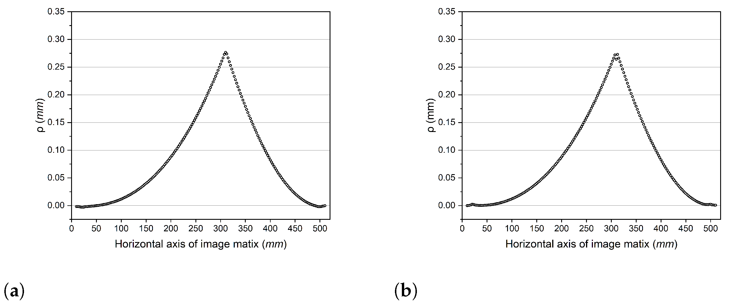
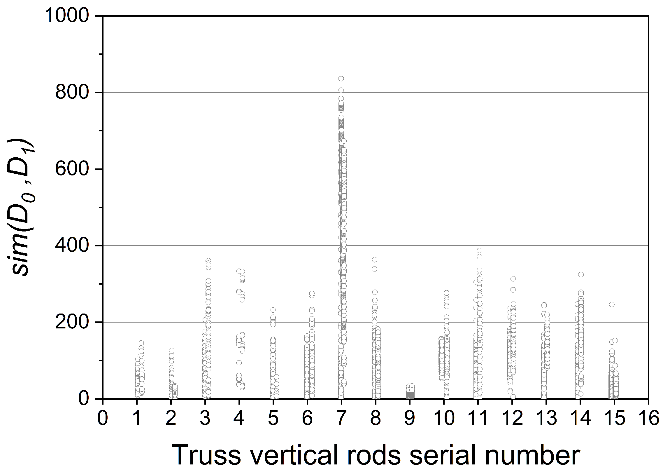
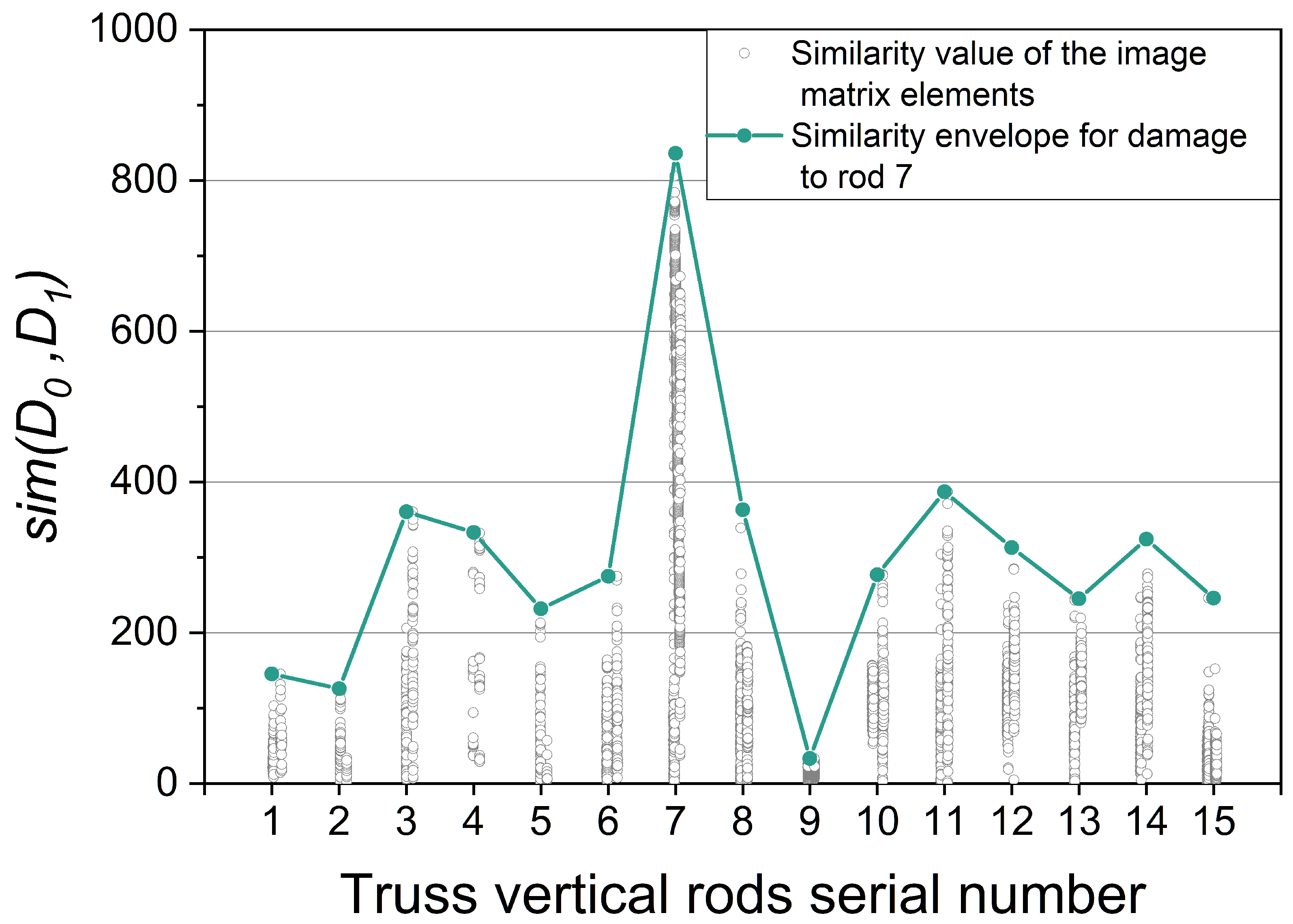
5.2.1. Single Damage Test Beam Image Matrix Similarity Analysis

Under 250 kN load condition, the lower edge curve of the test beam without damage and one rod damage (No. 7 rod) is extracted according to the previous method, and after noise reduction, the pixel coordinates of the lower edge curve form the image coordinate matrices $D_0$ and $D_1$. Then, the Euclidean distance of the homologous image points of the two image matrices is calculated using the Equation (6), whose calculation process is shown in Figure 40, and further the similarity $sim(D_0,D_1)$ distribution (Figure 41) is obtained by amplifying the damaged signal according to the Equation (7). To facilitate the view of the damage recognition effect, only the image matrix similarity results for the truss vertical rod regions are shown in Figure 41.

From Figure 41, the similarity peaks at vertical bar #7, indicating that damage is more likely to occur here than at other bars. By connecting the maximum similarity at each vertical bar, the similarity envelope of the test beam in the single damage condition can be obtained (Figure 42). The similarity envelope gives a more concise and obvious indication of the damage location.

Figure 42 shows that the image matrix similarity analysis method works well for single damage identification of the test beam and can accurately locate the damage location.

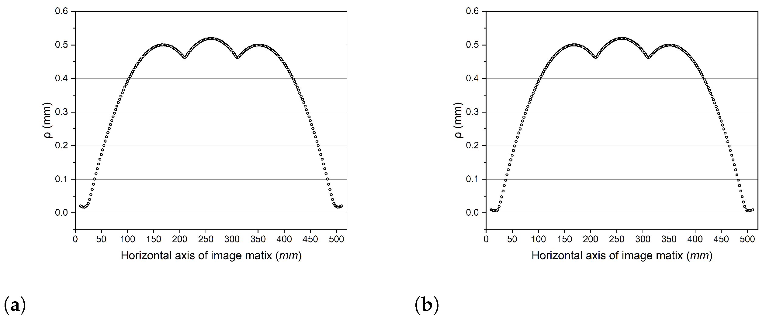
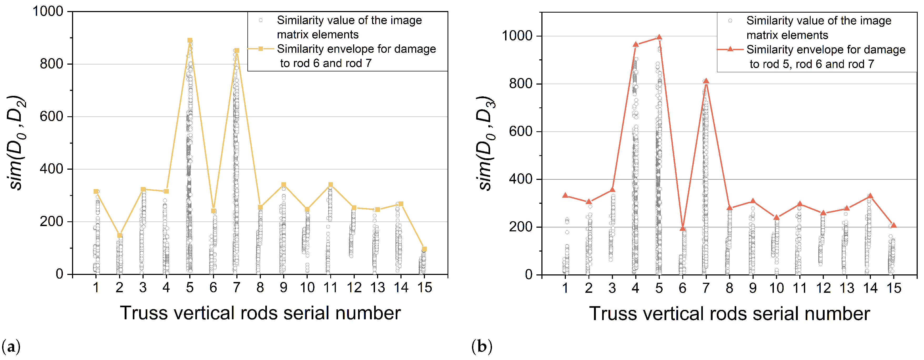
5.2.2. Multi-Damage Test Beam Image Matrix Similarity Analysis

The structural edge curves of two-bar damage (bars #5 and #7) and three-bar damage (bars #4, #5 and #7) under 250 kN load condition are selected, and the steps in Section 5.2.1 are repeated to obtain the image coordinate matrices $D_2$ and $D_3$. The similarity between them and the image matrices in the no damage condition is calculated respectively as shown in Figure 43.

To compare the image matrix similarity damage identification effects for different damage conditions, the similarity envelopes are integrated into the same coordinate system, as in Figure 44.

In summary, the analysis found that the test results are consistent with the results of the numerical simulations in Section 2.3, with the similarity ($sim$) envelope having a significant peak response at the damage location of the test specimen. This result indicates that the image matrix similarity analysis method proposed in this paper can accurately identify the damage locations on the test beams under each working condition and, at the same time, demonstrates that the overall deformation curve of the structure contains anomalous signals arising from local stiffness degradation caused by the damage.

6. Conclusions

Using digital image processing techniques, an image matrix similarity damage identification method for bridge structures is proposed based on the ability of images to describe the holographic deformation of structures. The test results show that the method can accurately identify the singular signal of local stiffness degradation caused by structural damage from the overall structural deformation and achieve the localization of damage. This solves the difficulty of damage identification due to incomplete test data and provides a new idea for beam damage identification. The research in this paper has engineering application prospects for small and medium-span bridges and for fast, economic, and efficient long-term health monitoring. The main conclusions of this paper are as follows.

(1) A digital orthophoto-based image matrix similarity damage identification method is proposed. Numerical simulation studies show that the damage will break the structural system deformation coordination, the abnormal distribution of pixels at the damage site will manifest odd signals in the matrix similarity test before and after the damage, the signal characteristics are shown as similarity curve discontinuity, and the discontinuity location is consistent with the damage site.

(2) A damage loading test of steel truss–concrete composite beam has been conducted, and the original test beam image is corrected by perspective transformation to obtain an equivalent digital orthophoto. Further, the holographic morphology of the test beams extracted by the SIFT feature extraction algorithm is verified, and the results show that the extracted morphology of the test beams is consistent with the real morphology of the structure.

(3) The lower edge curve of the experimental beam is affected by noise with regular oscillation, and the noise-containing curve is processed by the wavelet denoising function to obtain a continuous smooth lower edge curve of the structure. The validation results show that the maximum error of the noise-reduced curve is $3.42\%$.

(4) The image matrices of the structure before and after the damage are obtained from the coordinates of the lower edge curve. The similarity envelopes for each damage condition were derived by calculating the similarity of the image matrices under single damage condition and multiple damage conditions. The peak of the envelope is consistent with the position of the damaged rod, which verifies the accuracy of the damage position identification in practical applications.

References

1. Schlune, H.; Plos, M.; Gylltoft, K. Improved bridge evaluation through finite element model updating using static and dynamic measurements. Eng. Struct. 2009, 31, 1477–1485. [Google Scholar] [CrossRef]
2. Marinone, T.; Dardeno, T.; Avitabile, P. Reduced model approximation approach using model updating methodologies. J. Eng. Mech. 2018, 144, 04018005. [Google Scholar] [CrossRef]
3. Zhang, J.; Guo, S.; Wu, Z.; Zhang, Q. Structural identification and damage detection through long-gauge strain measurements. Eng. Struct. 2015, 99, 173–183. [Google Scholar] [CrossRef]
4. Cui, F.; Yuan, W.; Shi, J. Damage Detection of Structures Based on Static Response. J. Tongji Univ. 2000, 1, 8–11. [Google Scholar]
5. Xu, Z.D.; Li, S.; Zeng, X. Distributed strain damage identification technique for long-span bridges under ambient excitation. Int. J. Struct. Stab. Dyn. 2018, 18, 1850133. [Google Scholar] [CrossRef]
6. Banan, M.R.; Banan, M.R.; Hjelmstad, K. Parameter estimation of structures from static response. I. Computational aspects. J. Struct. Eng. 1994, 120, 3243–3258. [Google Scholar] [CrossRef]
7. Kourehli, S.S.; Bagheri, A.; Amiri, G.G.; Ghafory-Ashtiany, M. Structural damage detection using incomplete modal data and incomplete static response. KSCE J. Civ. Eng. 2013, 17, 216–223. [Google Scholar] [CrossRef]
8. Li, S.; Ma, L.; Tian, H. Structural damage detection method using incomplete measured modal data. J. Vib. Shock 2015, 34, 196–203. [Google Scholar]
9. He, R.S.; Hwang, S.F. Damage detection by a hybrid real-parameter genetic algorithm under the assistance of grey relation analysis. Eng. Appl. Artif. Intell. 2007, 20, 980–992. [Google Scholar] [CrossRef]
10. Savadkoohi, A.T.; Molinari, M.; Bursi, O.S.; Friswell, M.I. Finite element model updating of a semi-rigid moment resisting structure. Struct. Control Health Monit. 2011, 18, 149–168. [Google Scholar] [CrossRef]
11. Hua, J. Research on Bridge’S Damage Detection and Evaluation Based on Static Test Data; Southwest Jiaotong University: Chengdu, China, 2005. [Google Scholar]
12. Liu, G.; Mao, Z. Structural damage diagnosis with uncertainties quantified using interval analysis. Struct. Control Health Monit. 2017, 24, e1989. [Google Scholar] [CrossRef]
13. Yan, L. The Research of Suspension Bridge Damage Detection Based on the Grey Relation Theory and Genetic Algorithm; Lanzhou Jiaotong University: Lanzhou, China, 2015. [Google Scholar]
14. WenLong, G.; Jun, C.; DaShan, L. Structural damage identification based on quantum particle swarm optimization algorithm. J. Dyn. Control 2015, 13, 388–393. [Google Scholar]
15. Fang, Z.; Zhang, G.G.; Tang, S.H.; Chen, S.J. Finite element modeling and model updating of concrete cable-stayed bridge. China J. Highw. Transp. 2013, 26, 77–85. [Google Scholar]
16. Wang, Q.; Wu, N. Detecting the delamination location of a beam with a wavelet transform: An experimental study. Smart Mater. Struct. 2010, 20, 012002. [Google Scholar] [CrossRef]
17. Song, Y.Z.; Bowen, C.R.; Kim, H.A.; Nassehi, A.; Padget, J.; Gathercole, N.; Dent, A. Non-invasive damage detection in beams using marker extraction and wavelets. Mech. Syst. Signal Process. 2014, 49, 13–23. [Google Scholar] [CrossRef] [Green Version]
18. Ma, H.; Zhang, W.; Wang, Z. Application of wavelet analysis in cantilever beam crack identification. Chin. J. Comput. Mech. 2008, 05, 148–154. [Google Scholar]
19. XiaoWei, Y.; Tan, L.; ChuanZhi, D. Structural damage detection based on Kalman filter and neutral axis location. China J. Zhejiang Univ. (Eng. Sci.) 2017, 10, 137–143. [Google Scholar]
20. Pan, H.; Azimi, M.; Yan, F.; Lin, Z. Time-frequency-based data-driven structural diagnosis and damage detection for cable-stayed bridges. J. Bridge Eng. 2018, 23, 04018033. [Google Scholar] [CrossRef]
21. Fan, W.; Qiao, P. Vibration-based damage identification methods: A review and comparative study. Struct. Health Monit. 2011, 10, 83–111. [Google Scholar] [CrossRef]
22. Brownjohn, J.M.; De Stefano, A.; Xu, Y.L.; Wenzel, H.; Aktan, A.E. Vibration-based monitoring of civil infrastructure: Challenges and successes. J. Civ. Struct. Health Monit. 2011, 1, 79–95. [Google Scholar] [CrossRef]
23. Zheng, J.; Chen, D.; Hu, H. Boundary Adjusted Network Based on Cosine Similarity for Temporal Action Proposal Generation. Neural Process. Lett. 2021, 53, 2813–2828. [Google Scholar] [CrossRef]
24. Chu, X.; Zhou, Z.; Deng, G.; Duan, X.; Jiang, X. An overall deformation monitoring method of structure based on tracking deformation contour. Appl. Sci. 2019, 9, 4532. [Google Scholar] [CrossRef] [Green Version]
25. Wang, J.; Mao, Y.; Yan, T.; Liu, Y. Perspective Transformation Algorithm for Light Field Image. Laser Optoelectron. Prog. 2019, 56, 151003. [Google Scholar] [CrossRef]
26. Yuan, R.; Liu, M.; Hui, M.; Zhao, Y.; Dong, L. Depth map stitching based on binocular vision. Laser Optoelectron. Prog. 2018, 55, 282–287. [Google Scholar]
27. Jiang, J.; Zou, Y.; Yang, J.; Zhou, J.; Zhang, Z.; Huang, Z. Study on Bending Performance of Epoxy Adhesive Prefabricated UHPC-Steel Composite Bridge Deck. Adv. Civ. Eng. 2021, 2021, 6658451. [Google Scholar] [CrossRef]
28. Pinpin, L.; Wenge, Q.; Yunjian, C.; Feng, L. Application of 3D laser scanning in underground station cavity clusters. Adv. Civ. Eng. 2021, 2021, 8896363. [Google Scholar] [CrossRef]
29. Zhang, H.; Xia, J. Research on convergence analysis method of metro tunnel section–Based on mobile 3D laser scanning technology. IOP Conf. Ser. Earth Environ. Sci. 2021, 669, 012008. [Google Scholar] [CrossRef]
30. Wu, C.; Yuan, Y.; Tang, Y.; Tian, B. Application of Terrestrial Laser Scanning (TLS) in the Architecture, Engineering and Construction (AEC) Industry. Sensors 2022, 22, 265. [Google Scholar] [CrossRef]
31. Ling, X. Research on Building Measurement Accuracy Verification Based on Terrestrial 3D Laser Scanner. IOP Conf. Ser. Earth Environ. Sci. 2021, 632, 052086. [Google Scholar] [CrossRef]
32. Xi, C.X.; xiang Zhou, Z.; Xiang, X.; He, S.; Hou, X. Monitoring of long-span bridge deformation based on 3D laser scanning. Ingénierie Des Systèmes D’information 2018, 18, 113–130. [Google Scholar] [CrossRef]
33. Zhou, S.; Wu, X.; Qi, Y.; Luo, S.; Xie, X. Video shot boundary detection based on multi-level features collaboration. Signal Image Video Process. 2021, 15, 627–635. [Google Scholar] [CrossRef]
34. Hashimoto, R.F.; Barrera, J.; Ferreira, C.E. A Combinatorial Optimization Technique for the Sequential Decomposition of Erosions and Dilations. J. Math. Imaging Vis. 2004, 13, 17–33. [Google Scholar] [CrossRef]
35. Pillon, P.E.; Pedrino, E.C.; Roda, V.O.; do Carmo Nicoletti, M. A hardware oriented ad-hoc computer-based method for binary structuring element decomposition based on genetic algorithms. Integr. Comput. Aided Eng. 2016, 23, 369–383. [Google Scholar] [CrossRef]
36. Sussner, P.; Pardalos, P.M.; Ritter, G.X. On integer programming approaches for morphological template decomposition problems in computer vision. J. Comb. Optim. 1997, 1, 165–178. [Google Scholar] [CrossRef]
37. Deng, S.; Huang, Y. Fast algorithm of dilation and erosion for binary image. Comput. Eng. Appl. 2017, 53, 207–211. [Google Scholar]
38. Dokladalova, E. Algorithmes et Architectures Efficaces Pour Vision Embarquée. Ph.D. Thesis, Université Paris Est, Paris, France, 2019. [Google Scholar]
39. Chu, X.; Zhou, Z.; Deng, G.; Jiang, T.; Lei, Y. Study on Damage Identification of Beam Bridge Based on Characteristic Curvature and Improved Wavelet Threshold De-Noising Algorithm. Adv. Model. Anal. 2017, 60, 505–524. [Google Scholar] [CrossRef]
40. Tengjiao, J. Experimental Study on Damage Conditions of the Steel-Concrete Composite Beam Based on the Bridge Surface; Chongqing Jiaotong University: Chongqing, China, 2018. [Google Scholar]
41. Xi, C. Holographic Shape Monitoring and Damage Identification of Bridge Structure Based on Fixed Axis Rotation Photography; Chongqing Jiaotong University: Chongqing, China, 2020. [Google Scholar]
42. Andrade, L.C.M.D.; Oleskovicz, M.; Fernandes, R.A.S. Adaptive threshold based on wavelet transform applied to the segmentation of single and combined power quality disturbances. Appl. Soft Comput. 2016, 38, 967–977. [Google Scholar] [CrossRef]
43. Hu, Z.; Liu, L. Applications of wavelet analysis in differential propagation phase shift data de-noising. Adv. Atmos. Sci. 2014, 31, 825–835. [Google Scholar] [CrossRef]
Figure 1. Image matrix.
Applsci 12 03883 g001
Figure 2. Image matrix similarity analysis process; (a) Image matrix of damage-free structure; (b) Image matrix of damaged structure; (c) Matching tie point; (d) Euclidean distance of the homologous points.
Applsci 12 03883 g002
Figure 3. Finite element model of simply supported beam.
Applsci 12 03883 g003
Figure 4. Acquisition of finite element model image matrix; (a) the model nodes (red dots in the diagram) represent the non-zero elements of the image matrix; (b) image matrix for finite element models.
Applsci 12 03883 g004
Figure 5. Deflection diagram of X Z section for a single crack in a simply supported beam.
Applsci 12 03883 g005
Figure 6. Results of similarity analysis of single damage image matrix for simply supported beams; (a) Euclidean distance of the same name point on the upper edge of the model; (b) Euclidean distance of the same name point on the lower edge of the model.
Applsci 12 03883 g006
Figure 7. Location of the two cracks (eccentric situation).
Applsci 12 03883 g007
Figure 8. Results of similarity analysis of two eccentric damage image matrices for simply supported beams; (a) Euclidean distance of the homologous point on the upper edge of the model; (b) Euclidean distance of the homologous point on the lower edge.
Applsci 12 03883 g008
Figure 9. Location of the two cracks (Symmetrical situation).
Applsci 12 03883 g009
Figure 10. Results of matrix similarity analysis of two symmetrical damage images of simply supported beams; (a) Euclidean distance of the same name point on the upper edge of the model; (b) Euclidean distance of the same name point on the lower edge.
Applsci 12 03883 g010
Figure 11. Results of image matrix similarity analysis for various damage conditions; (a) single damage condition (position: x = 300 mm); (b) eccentric two damage condition (position: x = 300 mm & x = 400 mm); (c) symmetrical two damage condition (position: x = 200 mm & x = 300 mm).
Applsci 12 03883 g011
Figure 12. Steel truss–concrete composite beam for damage identification tests; (a) design dimensions of the test beam; (b) specimen entity.
Applsci 12 03883 g012
Figure 13. Arrangement of loading devices.
Applsci 12 03883 g013
Figure 14. Loading system of static load test.
Applsci 12 03883 g014
Figure 15. Location of loading and truss rod cutting.
Applsci 12 03883 g015
Figure 16. Test beam image without perspective transformation processing.
Applsci 12 03883 g016
Figure 17. Image perspective transformation model.
Applsci 12 03883 g017
Figure 18. Test beam image after perspective transformation process.
Applsci 12 03883 g018
Figure 19. Deflection gauge layout.
Applsci 12 03883 g019
Figure 20. Deflection meter measurement process under no-damage conditions.
Applsci 12 03883 g020
Figure 21. Basic parameters of Leica ScanStation P50 3D laser scanner.
Applsci 12 03883 g021
Figure 22. Layout of 3D laser scanning station.
Applsci 12 03883 g022
Figure 23. Layout of global sign points.
Applsci 12 03883 g023
Figure 24. Test beam scanning results.
Applsci 12 03883 g024
Figure 25. Test beam image feature points.
Applsci 12 03883 g025
Figure 26. Main features of test beam.
Applsci 12 03883 g026
Figure 27. Schematic diagram of edge point and noise point.
Applsci 12 03883 g027
Figure 28. Edge discontinuity of bridge structure image.
Applsci 12 03883 g028
Figure 29. Basic operation diagram of morphology; (a) open operation; (b) closed operation.
Applsci 12 03883 g029
Figure 30. Comparison before and after regression treatment of discontinuous edges of the test beam; (a) before; (b) after.
Applsci 12 03883 g030
Figure 31. Array arrangement of pixels in image.
Applsci 12 03883 g031
Figure 32. Pixel size calibration model.
Applsci 12 03883 g032
Figure 33. DOM obtained by 3D laser scanning of test beam.
Applsci 12 03883 g033
Figure 34. Direct contrast effect between image main shape and actual shape of test beam.
Applsci 12 03883 g034
Figure 35. Calculation method of height and spacing of vertical bar by 3D laser scanning.
Applsci 12 03883 g035
Figure 36. Edge extraction position.
Applsci 12 03883 g036
Figure 37. Original edge of the beam.
Applsci 12 03883 g037
Figure 38. The reasons for the oscillation effect of structural image edges.
Applsci 12 03883 g038
Figure 39. Lower edge curve of the test beam; (a) Original edge of the beam; (b) Edge curve after noise reduction.
Applsci 12 03883 g039
Figure 40. The calculation process of Euclidean distance in Equation (6).
Applsci 12 03883 g040
Figure 41. Single damage identification results of test beam.
Applsci 12 03883 g041
Figure 42. Single damage condition similarity envelope.
Applsci 12 03883 g042
Figure 43. Multi-damage condition similarity envelope; (a) two-damage conditions; (b) three-damage conditions.
Applsci 12 03883 g043
Figure 44. Similarity envelopes for all damage conditions.
Applsci 12 03883 g044