
Modeling and Simulation of Household Appliances Power Consumption


School of Industrial Engineering, University of Vigo, 36310 Vigo, Spain
*
Author to whom correspondence should be addressed.
Appl. Sci. 2022, 12(7), 3689; https://doi.org/10.3390/app12073689
Submission received: 23 February 2022
/
Revised: 20 March 2022
/
Accepted: 4 April 2022
/
Published: 6 April 2022
(This article belongs to the Topic Smart Electric Energy in Buildings)
Abstract
:Featured Application
The method presented in this paper serves to predict the consumption of household appliances by modeling their behavior and by simulating accordingly.
Abstract
The consumption of household appliances tends to increase. Therefore, the application of energy efficiency measurements is urgently needed to reduce the levels of power consumption. Over the last years, various methods have been used to predict household electricity consumption. As a novelty, this paper proposed a method of predicting the consumption of household appliances by evaluating statistical distributions (Kolmogorov–Smirnov Test and Pearson’s X2 test). To test the veracity of the evaluations, first, a set of random values was simulated for each hour, and their respective averages were calculated. These were compared with the averages of the real values for each hour. With the exception of HVAC during working days, great results were obtained. For the refrigerator, the maximum error was 3.91%, while for the lighting, it was 4.27%. At the point of consumption, the accuracy was even higher, with an error of 1.17% for the dryer while for the washing machine and dishwasher, their minimum errors were less than 1%. The error results confirm that the applied methodology is perfectly acceptable for modeling household appliance consumption and consequently predicting it. However, these consumptions can be only extrapolated to dwellings with similar surface areas and habitats.
1. Introduction
Currently, the growth in energy consumption and the need to address the pollution resulting from its generation are of concern to consumers and suppliers [1]. Governments have enacted legislation on circular economy and environmental protection [2,3]. Generally speaking, energy efficiency refers to both energy and climate policy [4]. Improving energy efficiency in buildings can significantly reduce the environmental impact of buildings as well as provide economic savings to consumers [5,6].
In residential buildings, household appliances consume a considerable amount of energy, resulting in high electricity bills [7]. This consumption has an increasing trend [8,9], despite improvements in their efficiency in recent years [10]. Households in the European Union account for 26% of the final energy consumption, yet their share in demand response (DR) systems is practically nonexistent [11]. Moreover, the energy consumption of refrigerators and freezers accounts for about half of the corresponding households [12], while HVAC is responsible for around 20–30% [13].
To cope with this high value of energy consumption, it can be of great help to predict or estimate how much each appliance may consume, i.e., its future behavior in those terms. An accurate prediction of the consumption at each hour of a day can be used to make decisions to try to reduce them as much as possible. In [14], an adaptive predictive control algorithm, using mixed linear programming, is proposed. Moreover, in [15], a two-stage control algorithm for the centralized management of residential loads is proposed to ensure their control. In [16], several regression models were established to analyze the determinants of end-use energy consumption. Further, in [17], a microgrid model was used to estimate the consumption of washing machines, dishwashers and dryers. Moreover, in [18], a model for detecting the behavior of building occupants was developed to estimate building consumption. In [19], three prediction models were proposed to estimate HVAC consumption as a function of occupants, electrical equipment and lighting. Similarly, in [20], a hidden Markov model was used to model a system and estimate the power values of household appliances. In [21], an SVM-based segmentation method was performed for dishwashers and washing machines. Moreover, in [22], a calibration method was employed to integrate POE data. In [23], a fuzzy logic controller was employed to estimate HVAC consumption. In [24], the authors establish a residential user evaluation system based on an evaluation model by selecting indicators related to user characteristics and electricity consumption data. In [25], an innovative customer preference-based appliance scheduling framework is presented. In [26], real-time simulations are provided by using finite element analysis programs. In [27], a multi-agent simulator capable of emulating different profiles of consumes and equipment is proposed. In [28], a harmonic coupled dynamic admittance matrix model based on voltage and current data was established to predict the consumption of household appliances. In [29], a domestic energy management model that was based on time perspective theory was developed, incorporating energy storage devices and flexible and smart appliances. In [30], the factors associated with the variation of total daily energy consumption by smart meters in different British households were investigated, including weather conditions, demographics and user attitudes. In [31], a study was conducted on the impact of teleworking in the aftermath of the COVID-19 pandemic on air-conditioning consumption using an ordinal logistic regression model. In [32], a real-time dynamic pricing method was proposed to determine the hourly electricity prices and schedule the electricity consumption of smart appliances. In [33], an equivalent thermal model of the HVAC system of a reference house was established. In [34], an air conditioner on/off state prediction model, combined with the diversity of occupant behavior, was established. In [35], Lasso regression was used to estimate the consumption of electrical appliances, electric heating, cooling and lighting of building parks in Wallonia. In [36], a Pecan Street dataset was used to group building occupants according to the energy they consume per electro-domestic appliance in their home with a subsequent load profile development. In [37], air-conditioning usage patterns of three climate zones were analyzed and developed. In [38], a thermal model was developed to calculate the regulating power provided by air conditioners. In [39], an optimal load control strategy for air conditioners was proposed. In [40], a model was established to characterize the Spanish electricity consumption considering typical appliances and key parameters of vulnerable households. In [41], a model of commonly used household appliances was constructed and a user satisfaction evaluation index was established. In [42], it was proposed to find the optimal delay time in the most energy-consuming equipment according to the priority of each appliance.
All of the above methodologies lack a descriptive statistical analysis of each household appliance for each hour of the day.
As alternatives to the previous solutions, this paper proposes an evaluation of the statistical distributions followed by each household appliance in a house [43] and, using them, to generate random values in such a way that they are as close as possible to the real values measured. To check the applicability of the assessment, it has been compared with an average of sets of simulated values with the sets of measured values and, thus, proves that the result is accurate.
All the above papers provide different forms of modeling, but none of them deal with the statistical distributions that may follow the consumptions at each period in depth. As a novelty, in this paper, the aim is to discover what statistical distribution the consumption of household appliances follows in 10-min periods, from the most basic ones (such as the normal, exponential or Weibull distribution) to the less known ones (Rayleigh or Generalized Pareto), applying the Kolmogorov–Smirnov test and the X2 test. To guarantee a correct evaluation, the averages of sets of random values are compared with the averages of real values for each hour, checking that the difference between them is acceptable.
Obtaining the statistical distribution of the power consumption of household appliances can be of certain interest because: it avoids dealing with errors, the absence of data or out-of-scale values; it may simulate data corresponding to one, three or even ten years in order to assess all possible scenarios; it can be statistically combined with other models in order to obtain more complex theoretical developments and, last but not least, derived results may be obtained from the type of distribution and its parameters (mean, mode, variance, quantiles, etc.).
This article is organized as follows: Section 2 describes the methodology applied for the two different types of consumption to deal with, i.e., the mathematical models and procedures used to obtain the results. Section 3 includes the information of the case study in detail. Section 4 presents the results after applying the methodology, together with a discussion of the results. Finally, Section 5 presents the conclusions of the work carried out.
2. Methodology
Based on the values of power consumption of different household appliances, they are processed according to the type of consumption; whether it is continuous for a long time or not.
2.1. Continuous Power Consumption Household Appliances
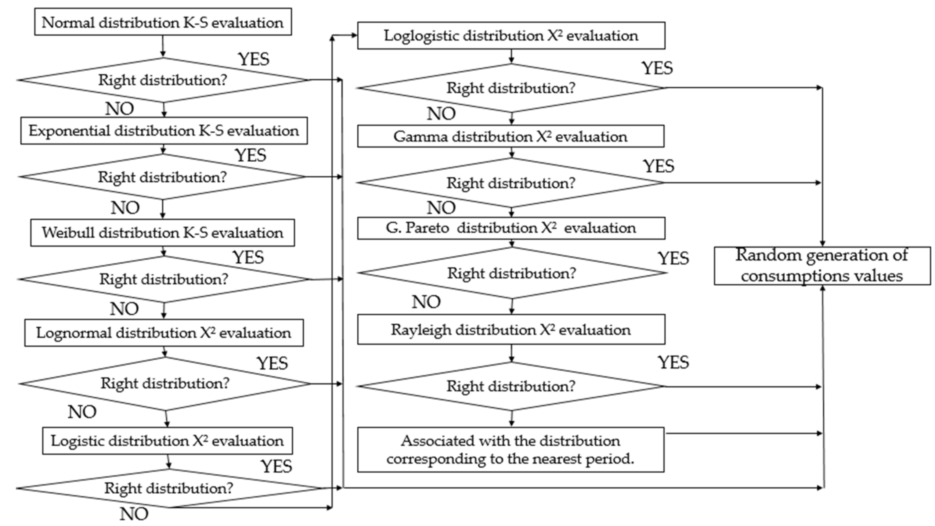
The starting data corresponds to each 10-min period of the day, from the one included in 00:00–00:10 to the one corresponding to 23:50–00:00. The distribution of consumption for each period is evaluated. First, every power consumption set of values will be evaluated using the Kolmogorov–Smirnov test [44] to check whether they follow a Normal distribution or not. First, the mean (μ) and standard deviation (σ) of each sample are calculated, and a theoretical normal cumulative distribution function, expressed in Equation (1), is used.
This theoretical cumulative function is compared with the observed cumulative frequency (). At first, the maximum upper difference () is obtained, as in Equation (2).
Subsequently, the maximum lower difference is calculated (), as it is expressed in Equation (3).
The maximum value between the upper difference and the lower difference is the maximum absolute difference () between the theoretical cumulative function and the observed cumulative frequency, as in Equation (4).
is compared with Dα, the maximum difference allowed according to the level of significance (α) and the type of distribution. Dα, Equation (5), is calculated by checking Table 1 and Table 2 for the values of and .
The significance selected for these distributions is 0.05 (95% of confidence). In Table 1, the coefficient of significance () is selected according to the model, its amount of data if the model is Weibull and the level of the significance. The significance selected for these distributions is 0.05 (95% of confidence).
In Table 2, the expression to calculate k(n) is selected according to the distribution, and subsequently, this last parameter is calculated with the amount of data. In this way, is calculated.
As it can be seen, in Table 2, the expression of k(n) is different in function of the distribution model, from Normal distribution to Weibull distribution.
In the case of D < Dα, the null hypothesis H0 of Normality is accepted so that the corresponding distribution would follow a Normal distribution. 10-min periods whose distribution rejects the null hypothesis of Normality are assessed in order to check if they follow an Exponential distribution with an analogous process to the previous one. The difference is the cumulative distribution function, expressed in Equation (6), where λ is the rate parameter, as well as the different values of cα and the way k(n) is calculated according to Table 2.
Again, it is checked for the Exponential distribution condition, and the unfitted sets are assessed against a Weibull distribution using the same process with its respective cumulative distribution function, formulated in Equation (7), where β is the scale factor and α is the shape factor.
The sets of values that are still not associated with any of the three distributions tested so far, will be subjected to an evaluation of the Lognormal, Logistic, Loglogistic, Gamma, Generalized Pareto and Rayleigh distributions until one of these is found to be correct. The method used for the last six mentioned distributions will be Pearson’s X2 test [45]. The process begins with the grouping of the data in a number of classes greater or equal to five, in such a way that they cover the whole possible range of values of the variables, and the expected frequency Oi is calculated for each sample.
Subsequently, the probability density function of the corresponding model is calculated. The Lognormal distribution is defined by Equation (8), while the Loglogistic distribution is as Equation (9), where µl is the location factor and s is the scale factor.
The Loglogistic, Gamma, Generalized Pareto and Rayleigh distributions are shown in Equations (10)–(13), respectively, where λa and αd are the skewness and distribution shape factors, respectively.
The probability density function of Loglogistic distribution is calculated by Equation (10):
Gamma distribution is defined by Equation (11):
Generalized Pareto distribution is expressed by Equation (12):
Finally, Equation (13) defines the Rayleigh distributions:
If any period corresponding to a series of values cannot be represented by any of the distributions assessed, it will be associated with the distribution corresponding to the nearest period, because the probability of being the same is quite high.
Once all the series values have an associated distribution, the expected frequency is calculated with the amount of data, defined in Equation (14).
Finally, X2, defined in Equation (15), is calculated and compared with X2α(k-r-1), where k is the number of classes and r is the number of parameters on which each distribution depends. If X2 is less than or equal to X2α(k-r-1) the null hypothesis H0 of the corresponding distribution to be evaluated is accepted.
Figure 1 shows a flowchart of the sequence of evaluations carried out before the following process.
Once all the curves have their associated distribution, a set of 300 random values are generated for each 10-min period according to their associated distribution, and the averages of these are compared with the averages of the real values to verify whether each simulation is close to reality (Figure 2).
The percentage of error in each case is calculated by Equation (16):
2.2. Discontinuous Power Consumption Household Appliances
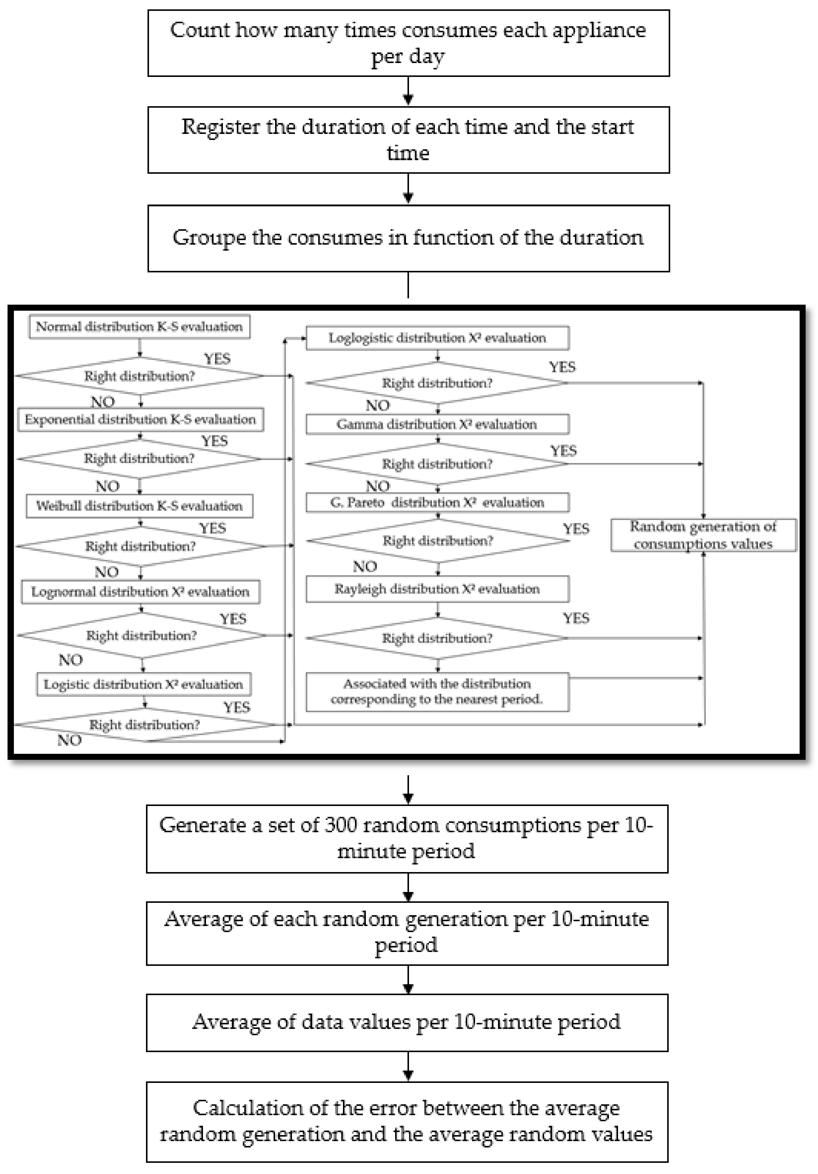
The number of times each household appliance is used per day is counted, as well as the duration of each time and in which periods of the day it happens.
The washing machine, dishwasher and dryer only consume energy while they are doing their functions. The first step consists of counting how many times each appliance consumes per day. The duration of each time and its start hour are registered as well.
The times with the same consumption duration are grouped together and evaluated in the same way as the continuous consumption appliances. The essential difference is that, in the latter case, just the moments where consumption is taking place are considered, and consequently shorter time intervals, whereas in the previous process the whole day was evaluated.
Once the power consumption curves are associated with each distribution, the following process is carried out:
- Simulation of the number of power consumptions of each element, where the probability of each integer value is based on the ratio of the previous count.
- If the above-simulated value is greater than or equal to 1, the duration of each count and its start time are simulated, also based on the data previously collected.
- Simulation of 300 sets of random consumptions according to the duration of the consumptions and their associated distribution, comparing their average value with the average of the real values.
- Calculation of the percentage of error by Equation (16).
Figure 3 shows a flowchart of the entire process of the treatment of the punctual consumptions, from the different counts to the calculation of errors, including the evaluation of distributions
The simulation was carried out with the consumption data of a house, with 199 m2 and three occupants, located in Vancouver. The extrapolation of results can be done in homes with an equivalent surface area, an equal number of inhabitants and a similar climatic zone. If these conditions change, the results would be different. Thus, if the surface area was larger, the consumption would increase. If it were a single dwelling, consumption would be lower, on the other hand. However, the methodology proposed in this paper can be applied if the number of consumption values available are significant and correspond to the same appliances that have been evaluated. Moreover, in some cases, such as the HVAC, the climate data influences the models obtained. This fact is not taken into account in this research work but can be of interest for future work.
3. Case study
The methodology explained in the previous section was applied to the instantaneous consumption data per second of different household appliances, extracted from [43], namely lighting, refrigerator, HVAC, dryer, washing machine and dishwasher.
The input data are the consumption of different household appliances in a house located in Vancouver. The powers were measured for 63 days, from 6 March 2016 to 7 May 2016. The dwelling consists of two floors, with a total of 199 m2 and three people living in it. Before starting the statistical evaluation, the consumption was grouped according to a 10-min period of power and then separated into three groups, i.e., working days, Saturdays and Sundays. The last step beforehand was to distinguish between continuous and discontinuous consumption, given that the treatment of the latter is more complex.
The reason for evaluating the 10-min periods is a matter of trade-off in accuracy and computational cost. On one hand, in a 10-min period, an appliance is not very likely to experience a large number of consumption changes. If it were 20 min, there is a risk of adding a larger error, as it could cover more than two phases of operation, e.g., a dishwasher. On the other hand, if the period is reduced to 5 min, the accuracy would increase, but the computational cost would be doubled, as twice as many periods would have to be modeled. Thus, a period of 10 min shows an adequate balance. The refrigerator, lighting and HVAC consume a considerable minimum at all times, while the dryer, dishwasher and washing machine only consume a considerable amount when they are running, thus they are considered point loads, or discontinuous consumptions.
A summary of the type of data can be observed in Table 3, with its type of consumptions, days and amount.
4. Results
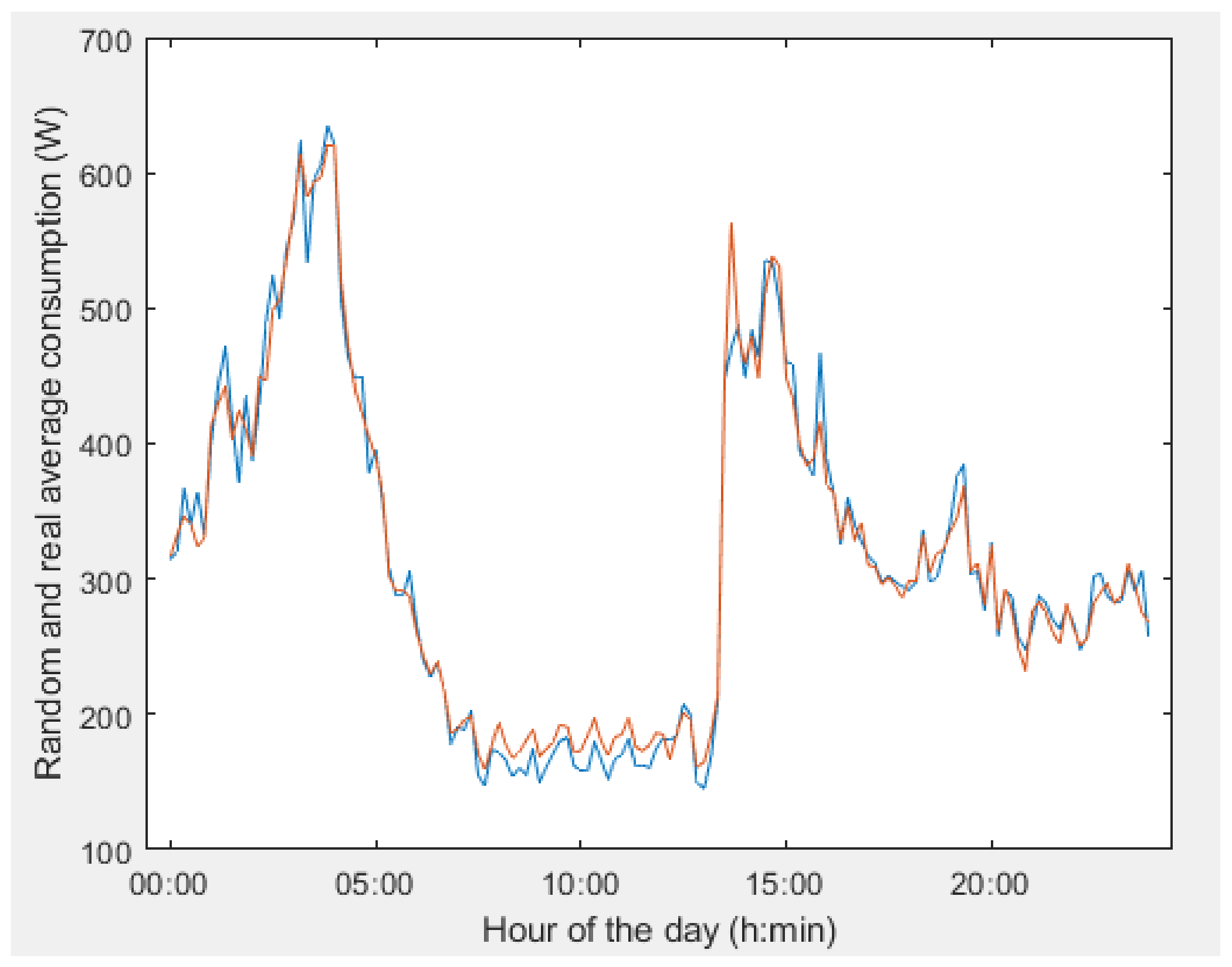
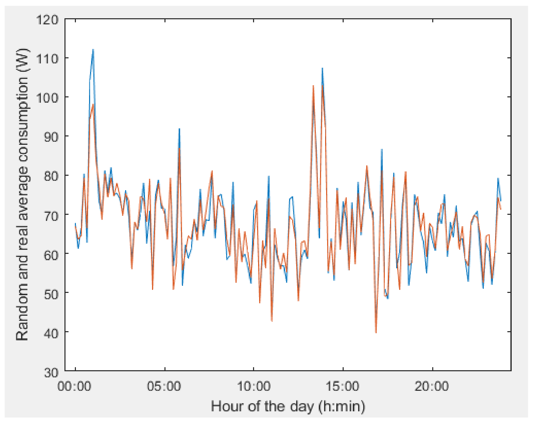
Figure 4 compares the simulated average values with the real average values for each 10-min period of lighting during the weekdays. In general, the trends in both graphs are very similar, since the off-peak hours, between 08:00 and 13:00, coincide, and the peak hours, around 07:00, are the same.
However, there are some significant differences between the simulation and the measured situation, especially at 15:00, just at the end of the hours of minimum consumption.
The error of the simulation with respect to the measured values is 3.81%, an acceptable value, which makes the simulation valid and perfectly close to the real situation.
Figure 5 shows the difference in lighting on Saturdays. Just as there are several more coinciding values in the previous graph, with the same trend, there are also two or three consumption peaks with a somewhat more significant difference than in the previous case, which means that the error increases to 4.26%, but it is still a valid simulation that is close to reality.
In the case of Sundays, there are also slightly unequal trends between the two curves (Figure 6), but also some significant differences in some specific points. The error produced in this simulation is 4.27%, very close to that of Saturdays thus all the simulations for the three lighting cases are acceptable.
In the case of the refrigerator during the days of the week (Figure 7), the same trend and generally insignificant differences can be seen, except for the first peak. In many cases, the values are practically the same or very close. The error is 3.91%, thus the simulation is considered successful.
On Saturdays (Figure 8), the simulation of refrigerator consumption is even tighter than on weekdays. Differences are generally minimal, leading to an error of 3.33%.
For Sundays (Figure 9), the same happens as with the simulations for Saturdays, with minimal deviations and a high coincidence. Nevertheless, the error amounts to 3.61%, which is not very significant. The three simulation graphs for the refrigerator consumption fit perfectly with a real situation.
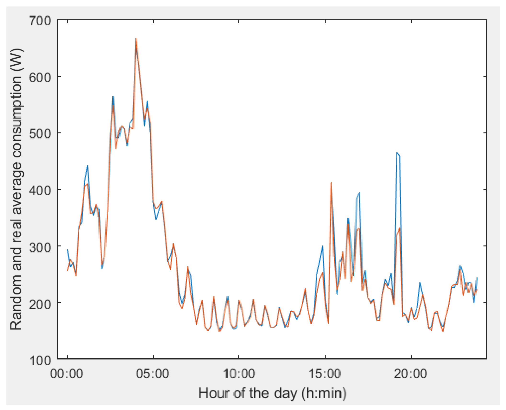
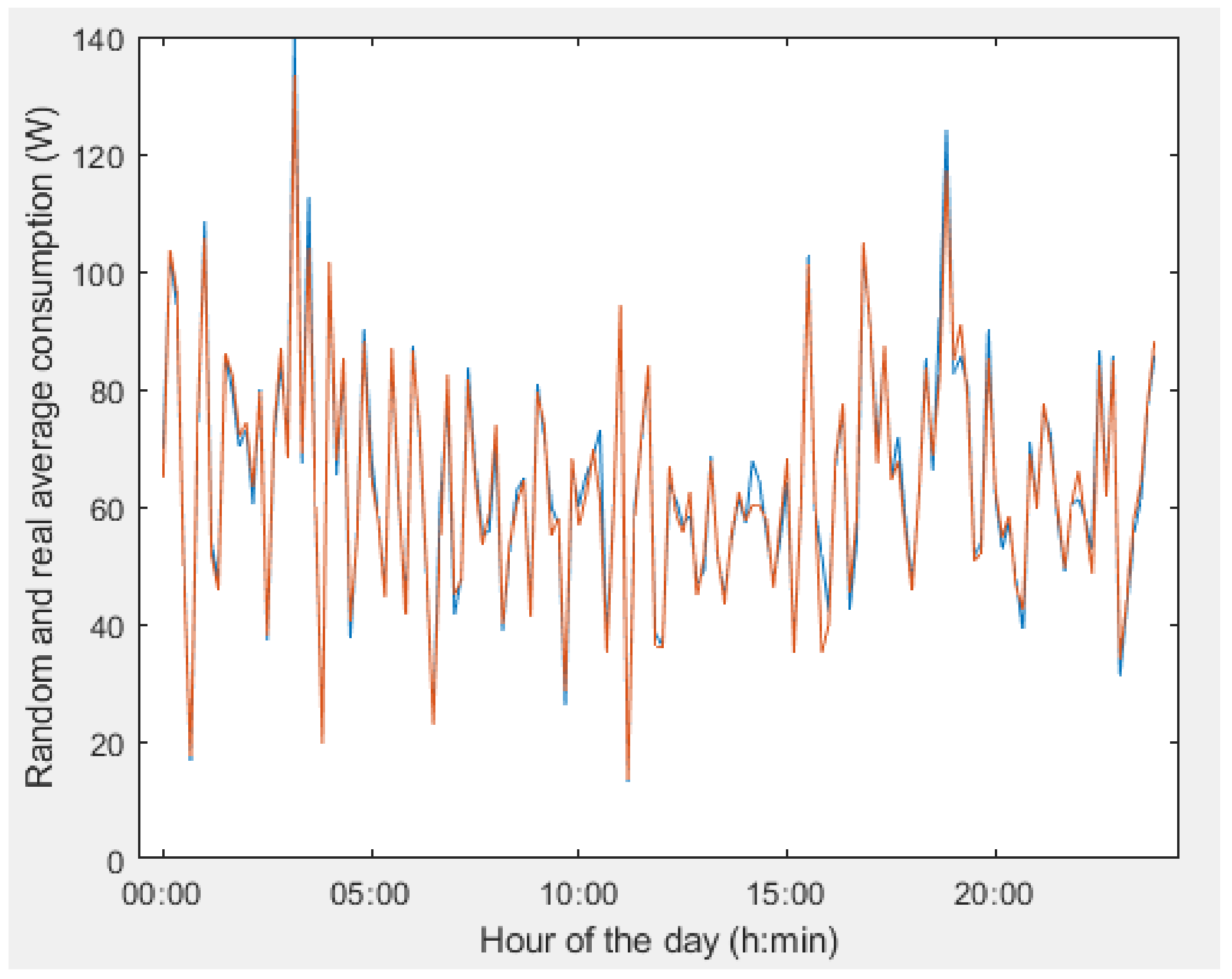
In the case of HVAC on weekdays (Figure 10), the same general trend between the simulation and the real values can also be observed, but in this case, there are more differences, although they are not particularly significant. These inaccuracies are responsible for an error of 5.55%, the highest error of all simulations.
For Saturdays (Figure 11), as well as a high number of ex-actual coincidences, there are also a few other considerably significant deviations. However, the error produced in this case is smaller than for weekdays and drops to 4.72%.
Finally, in the HVAC simulation for Sundays (Figure 12), the trends are practically the same and show a high number of coinciding values for weekdays and Sundays, and consequently a lower error (4.03%). The three HVAC simulations are also considered acceptable despite being the ones with the highest error.
In the case of the dryer during the days (Figure 13), the most frequent duration occurs with a 40 min consumption, as can be seen in the graph. In this case, the simulation is practically coincident with the real average, producing an error of 1.17%. The rest of the graphs with different durations have not been included, as they are very unlikely and therefore have low significance.
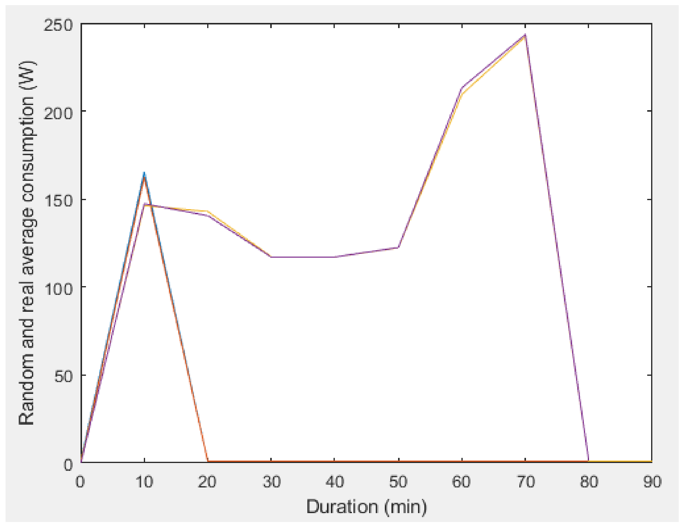
In the case of the washing machine during weekdays (Figure 14), the most frequent consumption durations are 10 and 70 min, approximately. In this case, the simulations are also close to the average of the real data, with errors of 1.04% and 0.78% for the 10-min and 70-min durations, respectively. Both errors are low and, therefore, valid.
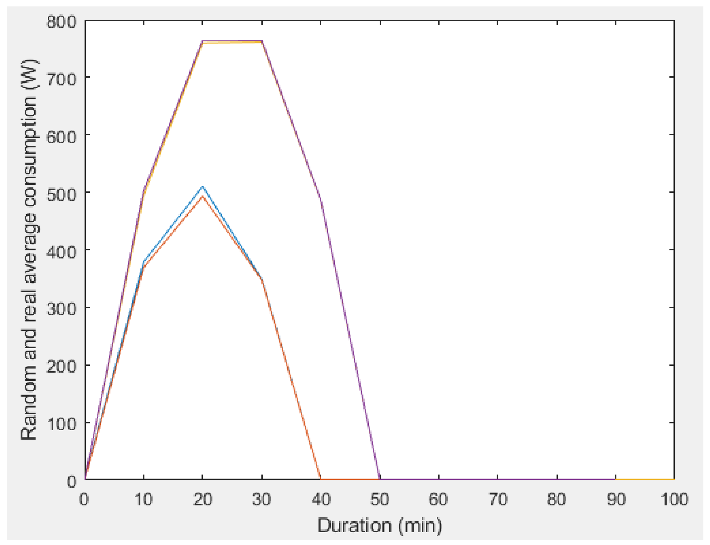
For the dishwasher during weekdays (Figure 15), 30 and 40 min were the most frequent durations. In the two cases, the errors (2.33% in 30 min and 0.78% in 40 min) are perfectively admissible, so the two approximations are also valid.
Table 4 shows a summary of the results obtained for each appliance, with the errors for each simulation.
After the results of the contrast of simulations, the applied methodology can be considered valid to predict the consumption of any home where the appliances are the same as those evaluated, i.e., lighting, HVAC, refrigerator, dryer, washing machine and dishwasher. Moreover, the results are perfectly extrapolated to homes whose surface area is equivalent to the one studied (199 m2) and the number of inhabitants is the same (three in this case). If these characteristics change, the results would no longer be applicable. However, the methodology can be applied in the same manner and, after a proper validation, the results obtained would be considered valid.
5. Conclusions
A ten minute period of consumption of six household appliances, based on the data provided, was assessed and simulated based on a related distribution. The first three appliances consume in a continuous way (lighting, refrigerator and HVAC), while the remaining appliances consume just in some periods of the day (dryer, washing machine and dishwasher). In order to establish the best model for each case, a methodology was proposed, which consisted of checking, in order of expectance, if data could be approximated through statistical distributions. The best results obtained, in the continuous consumption case, have been the refrigerator, then the lightning, and finally the HVAC. While the best results for the discontinuous consumptions were obtained for the washing machine, then the dryer, and the dishwasher.
The simulation of the continuous consumptions can be extrapolated to any house, as they are the most demanded appliances in most of them. For the dryer, washing machine and dishwasher, i.e., the discontinuous ones, their use can be very varied, since the duration can be longer or shorter. In these cases, it was decided to analyze the most frequent durations, as they are more significant. Generally speaking, good results were obtained and, therefore, simulation curves could also be extrapolated to other houses.
Author Contributions
Conceptualization, D.V. and D.S.-F.; methodology, D.V. and D.S.-F.; software, D.S.-F.; validation, D.V., E.M.-G. and A.F.-O.; formal analysis, E.M.-G. and A.F.-O.; investigation, D.S.-F.; resources, E.M.-G. and A.F.-O.; data curation, D.S.-F.; writing—original draft preparation, D.V. and D.S.-F.; writing—review and editing, E.M.-G. and A.F.-O.; visualization, A.F.-O.; supervision, D.V. and E.M.-G.; project administration, D.V. and A.F.-O. All authors have read and agreed to the published version of the manuscript.
Funding
This research received no external funding.
Institutional Review Board Statement
Not applicable.
Informed Consent Statement
Not applicable.
Data Availability Statement
Data analyzed in this research work was obtained from the link: https://github.com/smakonin/RAEdataset and the related information is described in Makonin, S.; Wang, Z.; Tumpach, C. «RAE: The rainforest automation energy dataset for smart grid meter data analysis», MDPI Data, vol. 3, no. 1, article 7, pp. 1–9 (2018).
Conflicts of Interest
The authors declare no conflict of interest.
Symbols and Acronyms
| μ | Mean |
| σ | Standard deviation |
| Normal cumulative distribution function | |
| Observed cumulative frequency | |
| Probability density function | |
| Upper difference between the observed cumulative frequency and normal cumulative Distribution | |
| Lower difference between the observed cumulative frequency and normal cumulative distribution | |
| Maximum difference between the observed cumulative frequency and normal cumulative distribution | |
| Maximum tabulated difference between the observed cumulative frequency and normal cumulative distribution | |
| Coefficient of significance | |
| Tabulated expression which determines | |
| Expected frequency | |
| Observed frequency | |
| α | Level of significance |
| n | Number of samples |
| λ | Rate parameter |
| β | Scale factor |
| α | Shape factor |
| μl | Location factor |
| λa | Skewness shape factor |
| αd | Distribution shape factor |
| X2 | Chi square |
| X2α(k-r-1) | Tabulated chi square |
| DR | Demand Response |
| HVAC | Heating, ventilating and air condition |
| SVM | Support-vector machines |
| POE | Post Occupancy Evaluation |
References
- Avila, M.; Méndez, J.; Ponce, P.; Peffer, T.; Meier, A.; Molina, A. Energy Management System Based on a Gamified Application for Households. Energies 2021, 14, 3445. [Google Scholar] [CrossRef]
- Guo, A.H. Research and Exploration on Green Design of Household Electrical Appliances. Adv. Mater. Res. 2014, 945–949, 531–534. [Google Scholar] [CrossRef]
- Lokeshgupta, B.; Sivasubramani, S. Dynamic Economic and Emission Dispatch with Renewable Energy Integration Under Uncertainties and Demand-Side Management. Electr. Eng. 2022, 1–12. [Google Scholar] [CrossRef]
- Kott, M. The electricity consumption in Polish households. In Proceedings of the 2015 Modern Electric Power Systems (MEPS), Proceedings of the International Conference on Modern Electric Power Systems, Wroclaw, Poland, 6–9 July 2015; IEEE: New York, NY, USA, 2016; pp. 1–5. [Google Scholar]
- Fattoruso, G.; De Vito, S.; Di Palma, C.; Di Francia, G. Innovative System and Method for Monitoring Energy Efficiency in Buildings. In Sensors; Springer: New York, NY, USA, 2013; Volume 162, pp. 523–527. [Google Scholar] [CrossRef]
- Mahmoudi, M.; Afsharchi, M.; Khodayifar, S. Demand Response Management in Smart Homes Using Robust Optimization. Electr. Power Components Syst. 2020, 48, 817–832. [Google Scholar] [CrossRef]
- Chauhan, R.K.; Chauhan, K.; Badar, A.Q. Optimization of electrical energy waste in house using smart appliances management System-A case study. J. Build. Eng. 2021, 46, 103595. [Google Scholar] [CrossRef]
- Villanueva, D.; Cordeiro, M.; Feijóo, A.; Míguez, E.; Fernández, A. Effects of Adding Batteries in Household Installations: Savings, Efficiency and Emissions. Appl. Sci. 2020, 10, 5891. [Google Scholar] [CrossRef]
- Mazzeo, D.; Baglivo, C.; Matera, N.; Congedo, P.M.; Oliveti, G. A novel energy-economic-environmental multi-criteria decision-making in the optimization of a hybrid renewable system. Sustain. Cities Soc. 2020, 52, 101780. [Google Scholar] [CrossRef]
- Toader, C.; Postolache, P.; Golovanov, N.; Porumb, R.; Mircea, I.; Mircea, P.-M. Power quality impact of energy-efficient electric domestic appliances. In Proceedings of the International Conference on Applied and Theoretical Electricity, Craiova, Romania, 23–25 October 2014; IEEE: New York, NY, USA, 2014; pp. 1–8. [Google Scholar]
- Amin, A.; Kem, O.; Gallegos, P.; Chervet, P.; Ksontini, F.; Mourshed, M. Demand response in buildings: Unlocking energy flexibility through district-level electro-thermal simulation. Appl. Energy 2021, 305, 117836. [Google Scholar] [CrossRef]
- Xu, Z.; Guo, N.; Wang, Y.; Yan, G. Identifying Fridge Consumption Non-intrusively. In Proceedings of the 3rd IEEE Conference on Energy Internet and Energy System Integration: Ubiquitous Energy Network Connecting Everything, Changsha, China, 8–10 November 2019; IEEE: New York, NY, USA, 2020; pp. 2770–2775. [Google Scholar]
- Liu, T.; Jin, L.; Zhong, C.; Xue, F. Study of thermal sensation prediction model based on support vector classification (SVC) algorithm with data preprocessing. J. Build. Eng. 2021, 48, 103919. [Google Scholar] [CrossRef]
- Colmenar-Santos, A.; Muñoz-Gómez, A.-M.; Rosales-Asensio, E.; Fernandez Aznar, G.; Galan-Hernandez, N. Adaptive model predictive control for electricity management in the household sector. Int. J. Electr. Power Energy Syst. 2022, 137, 107831. [Google Scholar] [CrossRef]
- Lankeshwara, G.; Sharma, R.; Yan, R.; Saha, T.K. Control algorithms to mitigate the effect of uncertainties in residential demand management. Appl. Energy 2021, 306, 117971. [Google Scholar] [CrossRef]
- Lee, S.-J.; Song, S.-Y. Determinants of residential end-use energy: Effects of buildings, sociodemographics, and household appliances. Energy Build. 2021, 257, 111782. [Google Scholar] [CrossRef]
- Hecht, C.; Sprake, D.; Vagapov, Y.; Anuchin, A. Domestic demand-side management: Analysis of microgrid with renewable energy sources using historical load data. Electr. Eng. 2021, 103, 1791–1806. [Google Scholar] [CrossRef]
- Lee, Y.; Yoon, Y.; Moon, H. Occupant behavior detection from environmental data and appliance electricity consumptions using machine learning. In Proceedings of the 16th Conference of the International Society of Indoor Air Quality and Climate: Creative and Smart Solutions for Better Built Environments, Indoor Air 2020, Virtual, Online, 1 November 2020; ISIAQ: Herndon, VA, USA, 2020. [Google Scholar]
- Liang, R.; Ding, W.; Zandi, Y.; Rahimi, A.; Pourkhorshidi, S.; Khadimallah, M.A. Buildings’ internal heat gains prediction using artificial intelligence methods. Energy Build. 2021, 258, 111794. [Google Scholar] [CrossRef]
- Hussein, N.; Hesham, A.; Rashawn, M. States and power consumption estimation for NILM. In Proceedings of the 14th International Conference on Computer Engineering and Systems, Cairo, Egypt, 17 December 2019; IEEE: New York, NY, USA, 2020; pp. 275–281. [Google Scholar]
- Wenninger, M.; Stecher, D.; Schmidt, J. SVM-based segmentation of home appliance energy measurements. In Proceedings of the 18th IEEE International Conference on Machine Learning and Applications, Boca Raton, FL, USA, 16–19 December 2019; IEEE: New York, NY, USA, 2020; pp. 1666–1670. [Google Scholar]
- Yu, C.; Du, J.; Pan, W. Improving accuracy in building energy simulation via evaluating occupant behaviors: A case study in Hong Kong. Energy Build. 2019, 202, 109373. [Google Scholar] [CrossRef]
- Parvin, K.; Al-Shetwi, A.Q.; Hannan, M.A.; Jern, K.P. Modelling of Home Appliances Using Fuzzy Controller in Achieving Energy Consumption and Cost Reduction. Electron. Electr. Eng. 2021, 27, 15–25. [Google Scholar] [CrossRef]
- Wang, Z.; Sun, M.; Gao, C.; Wang, X.; Ampimah, B.C. A new interactive real-time pricing mechanism of demand response based on an evaluation model. Appl. Energy 2021, 295, 117052. [Google Scholar] [CrossRef]
- Waseem, M.; Lin, Z.; Liu, S.; Zhang, Z.; Aziz, T.; Khan, D. Fuzzy compromised solution-based novel home appliances scheduling and demand response with optimal dispatch of distributed energy resources. Appl. Energy 2021, 290, 116761. [Google Scholar] [CrossRef]
- Mutluer, M. Analysis and Design Optimization of Permanent Magnet Motor with External Rotor for Direct Driven Mixer. J. Electr. Eng. Technol. 2021, 16, 1527–1538. [Google Scholar] [CrossRef]
- Mota, F.P.; Steffens, C.R.; Adamatti, D.F.; Botelho, S.S.D.C.; Rosa, V. A persuasive multi-agent simulator to improve electrical energy consumption. J. Simul. 2021, 1–15. [Google Scholar] [CrossRef]
- Xie, X.; Chen, D. Data-driven dynamic harmonic model for modern household appliances. Appl. Energy 2022, 312, 118759. [Google Scholar] [CrossRef]
- Dorahaki, S.; Rashidinejad, M.; Ardestani, S.F.F.; Abdollahi, A.; Salehizadeh, M.R. A home energy management model considering energy storage and smart flexible appliances: A modified time-driven prospect theory approach. J. Energy Storage 2022, 48, 104049. [Google Scholar] [CrossRef]
- McKenna, E.; Few, J.; Webborn, E.; Anderson, B.; Elam, S.; Shipworth, D.; Cooper, A.; Pullinger, M.; Oreszczyn, T. Explaining daily energy demand in British housing using linked smart meter and socio-technical data in a bottom-up statistical model. Energy Build. 2022, 258, 111845. [Google Scholar] [CrossRef]
- Toosty, N.T.; Hagishima, A.; Bari, W.; Zaki, S.A. Behavioural changes in air-conditioner use owing to the COVID-19 movement control order in Malaysia. Sustain. Prod. Consum. 2022, 30, 608–622. [Google Scholar] [CrossRef]
- Tehrani, M.; Nazar, M.S.; Shafie-Khah, M.; Catalao, J.P.S. Demand Response Program Integrated With Electrical Energy Storage Systems for Residential Consumers. IEEE Syst. J. 2022, 1–12. [Google Scholar] [CrossRef]
- Gong, H.; Jones, E.S.; Alden, R.; Frye, A.G.; Colliver, D.; Ionel, D.M. Virtual Power Plant Control for Large Residential Communities Using HVAC Systems for Energy Storage. IEEE Trans. Ind. Appl. 2021, 58, 622–633. [Google Scholar] [CrossRef]
- Yan, L.; Liu, M. Predicting household air conditioners’ on/off state considering occupants’ preference diversity: A study in Chongqing, China. Energy Build. 2021, 253, 1–17. [Google Scholar] [CrossRef]
- Nishimwe, A.M.R.; Reiter, S. Estimation, analysis and mapping of electricity consumption of a regional building stock in a temperate climate in Europe. Energy Build. 2021, 253, 111535. [Google Scholar] [CrossRef]
- Dongre, P.; Aldrees, A.; Gračanin, D. Clustering appliance energy consumption data for occupant energy-behavior modeling. BuildSys 2021. In Proceedings of the 2021 ACM International Conference on Systems for Energy-Efficient Built Environments, Coimbra, Portugal, 17–18 November 2021; ACM: New York, NY, USA, 2021; pp. 290–293. [Google Scholar]
- Liu, H.; Sun, H.; Mo, H.; Liu, J. Analysis and modeling of air conditioner usage behavior in residential buildings using monitoring data during hot and humid season. Energy Build. 2021, 250, 111297. [Google Scholar] [CrossRef]
- Hua, Y.; Xie, Q.; Hui, H.; Ding, Y.; Wang, W.; Qin, H.; Shentu, X.; Cui, J. Collaborative voltage regulation by increasing/decreasing the operating power of aggregated air conditioners considering participation priority. Electr. Power Syst. Res. 2021, 199, 107420. [Google Scholar] [CrossRef]
- Yang, Z.; Ding, X.; Lu, X.; Jing, J.; Gao, C. Inverter air conditioner load modeling and operational control for demand response. Dianli Xitong Baohu yu Kongzhi/Power Syst. Prot. Control 2021, 49, 132–140. [Google Scholar]
- Barrella, R.; Cosin, A.; Arenas, E.; Linares, J.I.; Romero, J.C.; Centeno, E. Modeling and analysis of electricity consumption in Spanish vulnerable households. In Proceedings of the 2021 IEEE Madrid PowerTech, Madrid, Spain, 28 June–2 July 2021; pp. 1–6. [Google Scholar] [CrossRef]
- Wang, Z.; Li, P.; Liu, Z.; Sun, P.; Yang, B. Research on Optimal Control Strategy of Household Electricity Load. In Proceedings of the 3rd Asia Energy and Electrical Engineering Symposium, Chengdu, China, 26–29 March 2021; IEEE: New York, NY, USA, 2021; pp. 765–771. [Google Scholar]
- Karamalian, D.; Moradian, M.; Heydari, S. Residential Energy Management Using Hierarchical Delay in Home Appliance. J. Electr. Syst. 2021, 17, 77–89. [Google Scholar]
- Makonin, S.; Wang, Z.J.; Tumpach, C. RAE: The Rainforest Automation Energy Dataset for Smart Grid Meter Data Analysis. Data 2018, 3, 8. [Google Scholar] [CrossRef] [Green Version]
- Kumar, R.; Kumar, A.; Shankhwar, A.K.; Verma, A.; Kumar, V. Modelling of metereological drought in the foothills of Central Himalayas: A case study in Uttarakhand State, India. Ain Shams Eng. J. 2022, 13, 1–14. [Google Scholar] [CrossRef]
- Babichev, S.; Yasinska-Damri, L.; Liakh, I.; Durnyak, B. Comparison Analysis of Gene Expression Profiles Proximity Metrics. Symmetry 2021, 13, 1812. [Google Scholar] [CrossRef]
Figure 1.
Flowchart of the sequence of statistical distributions evaluations.

Figure 2.
Flowchart of the comparison between random and real consumptions.

Figure 3.
Flowchart of the treatment of the punctual consumptions.

Figure 4.
Random (blue) and real (orange) average consumption of the lighting during working days.

Figure 5.
Random (blue) and real (orange) average consumption of the lighting during Saturdays.

Figure 6.
Random (blue) and real (orange) average consumption of the lighting during Sundays.

Figure 7.
Random (blue) and real (orange) average consumption of the refrigerator during working days.
Figure 7.
Random (blue) and real (orange) average consumption of the refrigerator during working days.

Figure 8.
Random (blue) and real (orange) average consumption of the refrigerator during Saturdays.

Figure 9.
Random (blue) and real (orange) average consumption of the refrigerator during Sundays.

Figure 10.
Random (blue) and real (orange) average consumption of HVAC during working days.

Figure 11.
Random (blue) and real (orange) average consumption of HVAC during Saturdays.

Figure 12.
Random (blue) and real (orange) average consumption of HVAC during Sundays.

Figure 13.
Random (blue) and real (orange) average consumption of the dryer whose duration is 40 min during working days.
Figure 13.
Random (blue) and real (orange) average consumption of the dryer whose duration is 40 min during working days.

Figure 14.
Random (blue and yellow) and real (orange and purple) averages consumption of the washing machine, whose durations are 10 and 70 min during working days.
Figure 14.
Random (blue and yellow) and real (orange and purple) averages consumption of the washing machine, whose durations are 10 and 70 min during working days.

Figure 15.
Random (blue and purple) and real (red and orange) averages consumption of the dishwasher whose durations are 30 and 40 min during working days.
Figure 15.
Random (blue and purple) and real (red and orange) averages consumption of the dishwasher whose durations are 30 and 40 min during working days.


Table 1.
Cα values according to the model and the significance.
| A | |||
|---|---|---|---|
| Model | 0.1 | 0.05 | 0.01 |
| General | 1.224 | 1.358 | 1.628 |
| Normal | 0.819 | 0.895 | 1.035 |
| Exponential | 0.990 | 1.094 | 1.308 |
| Weibull n = 10 | 0.760 | 0.819 | 0.944 |
| Weibull n = 20 | 0.779 | 0.843 | 0.973 |
| Weibull n = 50 | 0.790 | 0.856 | 0.988 |
| 0.803 | 0.874 | 1.007 | |
Table 2.
k(n) according to the distribution function.
| Distribution | k(n) |
|---|---|
| General | |
| Normal | |
| Exponential | |
| Weibull |
Table 3.
Summary of the evaluated appliances with their type of consumption, type of days and amount of data.
Table 3.
Summary of the evaluated appliances with their type of consumption, type of days and amount of data.
| Appliance | Type of Consumption | Type of Days | Amount of Data |
|---|---|---|---|
| Lightning | Continuous | Working days | 45 |
| Saturdays | 9 | ||
| Sundays | 9 | ||
| Refrigerator | Continuous | Working days | 45 |
| Saturdays | 9 | ||
| Sundays | 9 | ||
| HVAC | Continuous | Working days | 45 |
| Saturdays | 9 | ||
| Sundays | 9 | ||
| Dryer | Occasional | Working days | 45 |
| Washing machine | Occasional | Working days | 45 |
| Dishwasher | Occasional | Working days | 45 |
Table 4.
Summary of the error values.
| Appliance | Type of Day | Duration | Error |
|---|---|---|---|
| Lightning | Working day | All day | 3.81% |
| Saturdays | All day | 4.26% | |
| Sundays | All day | 4.27% | |
| Refrigerator | Working day | All day | 3.91% |
| Saturdays | All day | 3.33% | |
| Sundays | All day | 3.61% | |
| HVAC | Working day | All day | 5.55% |
| Saturdays | All day | 4.72% | |
| Sundays | All day | 4.03% | |
| Dryer | Working days | 40 min | 1.17% |
| Washing machine | Working days | 10 min | 1.04% |
| 70 min | 0.78% | ||
| Dishwasher | Working days | 30 min | 2.33% |
| 40 min | 0.78% |
Publisher’s Note: MDPI stays neutral with regard to jurisdictional claims in published maps and institutional affiliations. |
© 2022 by the authors. Licensee MDPI, Basel, Switzerland. This article is an open access article distributed under the terms and conditions of the Creative Commons Attribution (CC BY) license (https://creativecommons.org/licenses/by/4.0/).
Share and Cite
MDPI and ACS Style
Villanueva, D.; San-Facundo, D.; Miguez-García, E.; Fernández-Otero, A. Modeling and Simulation of Household Appliances Power Consumption. Appl. Sci. 2022, 12, 3689. https://doi.org/10.3390/app12073689
AMA Style
Villanueva D, San-Facundo D, Miguez-García E, Fernández-Otero A. Modeling and Simulation of Household Appliances Power Consumption. Applied Sciences. 2022; 12(7):3689. https://doi.org/10.3390/app12073689
Chicago/Turabian StyleVillanueva, Daniel, Diego San-Facundo, Edelmiro Miguez-García, and Antonio Fernández-Otero. 2022. "Modeling and Simulation of Household Appliances Power Consumption" Applied Sciences 12, no. 7: 3689. https://doi.org/10.3390/app12073689
Note that from the first issue of 2016, this journal uses article numbers instead of page numbers. See further details here.