A Deep Reinforcement Learning-Based Scheme for Solving Multiple Knapsack Problems

Abstract

A knapsack problem is to select a set of items that maximizes the total profit of selected items while keeping the total weight of the selected items no less than the capacity of the knapsack. As a generalized form with multiple knapsacks, the multi-knapsack problem (MKP) is to select a disjointed set of items for each knapsack. To solve MKP, we propose a deep reinforcement learning (DRL) based approach, which takes as input the available capacities of knapsacks, total profits and weights of selected items, and normalized profits and weights of unselected items and determines the next item to be mapped to the knapsack with the largest available capacity. To expedite the learning process, we adopt the Asynchronous Advantage Actor-Critic (A3C) for the policy model. The experimental results indicate that the proposed method outperforms the random and greedy methods and achieves comparable performance to an optimal policy in terms of the profit ratio of the selected items to the total profit sum, particularly when the profits and weights of items have a non-linear relationship such as quadratic forms.

1. Introduction

A knapsack problem is one of combinatorial optimization problems. Extending the single knapsack problem, the multiple knapsack problem (MKP) is a problem that finds disjoint subsets to maximize the total profit in knapsacks. In a nutshell, each subset can be distributed to different knapsacks, as long as the total weight of each subset is equal to or less than the capacity of the corresponding knapsack. MKP is formulated as follows:

$$\begin{array}{cc}\hfill & \underset{x}{max}\sum _j\sum _i{p}_i{x}_{ij}\hfill \\ \hfill & \mathrm{subject}\mathrm{to}\sum _i{w}_i{x}_{ij}\le c_j,\sum _j{x}_{ij}\le 1\hfill \\ \hfill & \mathrm{for}\forall i\in I,\forall j\in J,x_{ij}\in \{0,1\}\hfill \end{array}$$

(1)

where J is the pool of knapsacks, I is the pool of items, $p_i$ is the profit of the i-th item, $w_i$ is the weight of the i-th item, and $x_{ij}$ is a decision variable to indicate whether the i-th item is selected to be put in the j-th knapsack. The exact method has the computational complexity of $O\left({(J+1)}^{\left|I\right|}\right)$.

MKP arises in substantial real-world cases like vehicle/container loading, production scheduling, and resource allocation in the computer network systems [1,2]. Lahyani et al. [2] formulated production scheduling as MKP. It deals with assigning items to a period of the production schedule to maximize the profit of production and minimize the cost keeping the constraint of capacities. Kumaraguruparan et al. [3] formulated scheduling appliances as MKP in smart grid infrastructure. To minimize electricity bills in a household, it considers an appliance as an item, its energy consumption as weight, and the time period as a knapsack. Ketyko et al. [4] formulated a multi-user computation offloading problem as MKP. To maximize the profit of user equipment, it considers user equipment as items, requested CPU as weights, and CPU capacities of mobile edge computing server as capacities of knapsacks. Cappanera et al. [5] formulated Virtual Network Functions (VNF) placement problems as MKPs. It considers a data center as a knapsack, a service request as an item, and the quantity of the service requests as weight. Then, it solves the problem to maximize the total priority level of the requests. In various application fields, solving MKP with high performance in practical time to maximize revenue is unavoidable.

In MKP, there is a trade-off between empirical performance and reduced computational complexity. Note that MKP is an NP-hard problem [6]. Traditional approaches, such as heuristic or genetic algorithms, focus on reducing their computational complexity. These days, the development of deep neural network (DNN) accelerates the application of Machine Learning (ML) to various engineering problems. Reinforcement Learning (RL), one type of ML, is an experience-driven method that makes autonomous agents solve decision-making problems [7]. Deep reinforcement learning (DRL) has been applied not only to robot movement [8] and games such as AlphaGo [9] but also to discrete combinatorial optimization problems [10,11,12,13,14,15]. DRL agents trained with DNN can solve the high dimensional problems in a reasonable amount of time [2,16,17]. Recently, traveling salesman problem (TSP) and knapsack problem have been solved not only with supervised learning [10,18], but also with RL [11,19]. DRL with experience replay can be applied to the MKP problem because it can deal with various combinations of items and knapsacks in real-time without predefined massive data for training. In the literature, there are some approaches that solve a single knapsack problem, but there are lack of approaches for MKPs [10,11,19].

In this paper, we propose a DRL-based method to solve MKP. The proposed DRL method solves MKP by exploiting an existing Markov Decision Process (MDP) model for single knapsack problem in [11] and devising a novel capacity-aware knapsack selection method for MKP. Each state represents a separate problem state, and the agent’s action decides which item to be mapped to a knapsack with the greatest capacity. As a result, the proposed method makes a solution for an MKP by combining sequential actions made by an agent in each state. Our main contributions are as follows:

• We propose a DRL-based method to solve MKP, in which the DNN model is extensively trained with various combinations of random items and knapsacks. The trained single DNN model has the capability of solving diversified MKPs with untrained instance sets of items and knapsacks.
• We simplify the action space for MKP to make it possible to train the model in a scalable manner. The proposed method combines greedy sorting algorithms with the DRL training process, and the size of the action space is fixed to the number of items regardless of the number of knapsacks. It simplifies state transition pattern so that the agent can identify a change in the environment quickly during the training process.
• We adopt the Asynchronous Advantage Actor-Critic (A3C) [20] to expedite the learning process for DNN model. The training is performed asynchronously with multiple learners. A global model is shared with each learner, which contributes to the global model updating at the end of each episode.
• The experiments show that the DNN model can be successfully trained in a variety of configurations in terms of the number and capacity of knapsacks, and the number, weight, and profit of items. It is demonstrated that even when the weight and profits of items have a nonlinear relationship, the proposed method achieves comparable performance to an optimal policy.

The remainder of this article is organized as follows. In Section 2, we will summarize existing work on knapsack problems. In Section 3, we introduce a DRL method with a sorting algorithm for solving MKP. Section 4 compares our method with other baseline methods by evaluating computational results on random, linear, and quadratic instances. Finally, we conclude this paper in Section 5.

2. Related Work

2.1. Conventional Algorithms for Knapsack Problems

To reduce the complexity of an exact algorithm, heuristic algorithm and evolutionary algorithm solve single or multiple knapsack problems in a relaxed and greedy manner.

2.1.1. Exact Algorithms and Heuristic Algorithms

Martello and Toth proposed MTM, which is a branch and bound-based exact algorithm. The process of MTM includes surrogate relaxation and lower bounds which find an optimal solution heuristically for the current single knapsack one by one [6]. Mulknap is a branch and bound-based exact method proposed by Pisinger, which employs surrogate relaxation for upper bounds and the subset-sum problem for lower bounds. [21]. Martello and Toth proposed MTHM, which is introduced as a polynomial-time approximate solution. The summed process is composed of greedy mapping, rearrangement using reordering, swapping items between two knapsacks, replacing one item with a subset of unassigned items. It derives the computational complexity $O\left(\right|I{|}^2)$ [6]. For solving setup MKP, Lahyani et al. [2] proposed a matheuristic method. It generates heuristic-based solutions and tabu lists using period and class exchange. Dell’Amico et al. [22] developed a hybrid exact algorithm which combines Mulknap with decomposition method. It calls Mulknap algorithm (branch and bound-based algorithm) for $\tau$ seconds and iterates decomposition $\nu$ times.

2.1.2. Genetic Algorithm and Evolutionary Algorithm

Genetic algorithm (GA) is a representative approach to get a local optima using random search. The basic process of GA is as follows: (1) initially generate random solutions (2) evaluate solutions by their fitness value (3) select two parent solutions (4) regenerate solutions using genetic operator (crossover, mutation) [23]. Khuri et al. [24] used GA to solve 0/1 MKP. It generates initial random solutions and employs genetic operators (selection, crossover, and mutation) proportionally. The algorithm comes up with a solution toward maximizing fitness value which is total profit minus overfilled weights. Falkenauer [25] proposed the Grouping Genetic Algorithm (GGA) to solve bin packing problems. In GGA process, it initially generates population using copy and crossover. Fukunaga [26] proposed UGGA, which iteratively calls Fillundominated in the initialization stage of GGA. Fillundominated is an algorithm that finds an item to replace a subset of a knapsack with the same or greater weight than the subset’s total weight and the same or greater profit than the subset’s total profit. Kim and Han proposed Quantum-inspired Evolutionary Algorithm (QEA) to solve a single knapsack problem. QEA can generate a diversified population because Q-bit has a linear superposition of binary states [27]. In the process, the algorithm observes the state of quantum bits and iteratively compares the current solution with the previous.

2.2. Combinatorial Optimization with ML

Machine learning’s approximation reduces large amounts of calculations in decision-making problems. Various types of DNN based approaches such as Convolutional Neural Network (CNN) and Recurrent Neural Network (RNN) have been applied to solving a variety of optimization problems.

2.2.1. Combinatorial Optimization Problem (COP) with Pointer Network

Vinyal et al. [18] introduced pointer networks with RNNs to solve geometric problems. Two separated Long Short-Term Memory models (LSTM) RNNs are used; one is an encoder that encodes input sequence and the other is a decoder that derives output’s probability sequentially. Therefore, it can be applied to a problem in which output length depends on the length of the input sequence, such as selecting a point to visit at each time from a set number of points to visit. Bello et al. [19] applied pointer networks to A3C method to solve not only TSP but also single knapsack problems. The output of the decoder selects an item in each iteration time. The experiments for single knapsack problems use instances with fixed capacity in both training and test. Gu et al. [10] used pointer networks to solve single knapsack problems. Each Pointer is considered as an item and 0 indexed pointer means the end of the selected item. It employed a supervised loss function with a cross-entropy objective. Hu et al. employed pointer networks and DRL to solve 3D bin packing problems. The experiment result showed that the solution of the proposed method has the smallest surface area when compared to heuristics [28].

2.2.2. COP with Supervised/Unsupervised Learning

Rezoug et al. [29] proposed a supervised learning-based model to solve multidimensional knapsack problems. The proposed model is updated close to the optimal. It uses multiple regression including K-Nearest Neighbor (KNN) and Bayesian Automatic Relevance Determination (ARD). The model trained with small instances could solve the problem with large instances. Garcia et al. [30] designed unsupervised learning KNN to solve multidimensional knapsack problems. The designed method is a hybrid solution of KNN and metaheuristics, which are Particle Swarm Optimization (PSO) and Cuckoo Search (CS).

2.2.3. COP with DRL in MDP

Dai et al. [13] used structure2vec to solve COP in a weighted graph environment with tagged node state and partial tour length reward to reinforce the policy. Laterre et al. [31] formulated the process of solving bin packing problems as MDP process with DRL. The objective function is to minimize the cost. When items are all placed, then it gets 1 over cost as a reward and a reward buffer measures it by comparing the current reward with the best reward. The ranked reward is determined based on the evaluation, and it causes finding out a solution that outperforms the previous one. Olyvia et al. [14] used the Double Deep Q Network (DDQN) algorithm to solve a 2D bin packing problem. To get maximized empty space, it reinforces agent according to reward, which is either cluster size × compactness or a negative constant. The evaluation shows an increase in efficiency and decrease of loss according to the increase of learning iteration. Afshar et al. [11] proposed a state aggregation method to solve a single knapsack problem in MDP with Advantage Actor-Critic (A2C) algorithm. The result shows the proposed method outperforms other methods without aggregation. Zhang et al. [15] use the attention model to solve Dynamic Traveling Salesman Problem (DTSP). In DTSP the salesman decides the cities to visit on the travel while new customers can appear dynamically. Zhang proposed a DRL framework in an MDP where an agent model is composed of an encoder and a decoder and states are combined with static state and dynamic state.

3. Proposed Method

3.1. Actor Critic Background

In RL, an agent in a given state selects an action, and the environment returns reward and next states to the agent. State, action, reward, and next state sets from time t are used in MDP and can be denoted as the following form: $(s_t,a_t,r_t,s_{t+1})$. The continuous set $(s_t,a_t,r_t,s_{t+1})$ of an episode is called a trajectory. The return value of a trajectory can be denoted as $R={\sum }_{t=0}^{T-1}{\gamma }^t{r}_{t+1}$. $\gamma$ is a discount factor less than 1, and $r_{t+1}$ is a reward caused by action in time t. The action in a state is determined by a policy which can be deterministic or stochastic. The goal of RL is to find a policy which maximizes the return value. A value function is a key role estimating how good the transition from a given state to the target state is. The value function at $s_{t+1}$ gets the expected accumulated reward from $s_{t+1}$ to the end of the episode, and it can be denoted by $V\left(s_{t+1}\right)=\mathbb{E}\left[R_{t+1}\right]$.

There are two representative RL methods for a policy of an agent; value-based and policy-based. In a value-based learning, the policy is determined by the value functions. The estimation of the value function in a certain state is derived by updating it using the expected return values of the candidate states from the very next step. As a result, many iterations are required to get a converged expected accumulated reward at the first time step. Compared to the previous method, policy-based learning allows the policy to converge quickly without many iterations using a converged expected accumulated reward. One of policy-based learning, the policy gradient (PG) method directly updates the policy which has differential parameters toward maximizing the expected return value as follows:

$$J\left(\theta \right)={\mathbb{E}}_{{\pi }_{\theta }}\left[R_0\right]$$

(2)

$${\nabla }_{\theta }\left(J\right)={\mathbb{E}}_{{\pi }_{\theta }}\left[{\nabla }_{\theta }\right|R_{t}log{\pi }_{\theta }(a_t,s_t)]$$

(3)

In (2), ${\pi }_{\theta }$ denotes the policy of the action following parameterized vector $\theta$. The objective function $J\left(\theta \right)$ is equal to the expected return value got by ${\pi }_{\theta }$ at time 0. To find ${\pi }_{\theta }$ maximizing $J\left(\theta \right)$ is the fundamental goal. In (3), ${\nabla }_{\theta }\left(J\right)$ is the partial derivative of $J\left(\theta \right)$ in (2) with respect to $\theta$. $R_t$ is the return value in time t. By utilizing log-derivative trick, the sampled return value from an episode is directly used to update the policy, and it can cause the increase of the variance. An actor-critic algorithm can reduce the variance by substituting the estimated value per step. The estimated value can approximate a baseline and it can be denoted as $V_{{\theta }_V}\left(s_t\right)\approx b\left(s_t\right)$. The actor indicates a policy updated by PG method, and the critic is an approximated value, which estimates the return value by the actor.

3.2. System Model

Our work proposes state, action, and reward in MDP for solving an MKP by referring to and modifying parts of the existing work [11]. The state transition is deterministic here and the next state is decided by the current state and action.

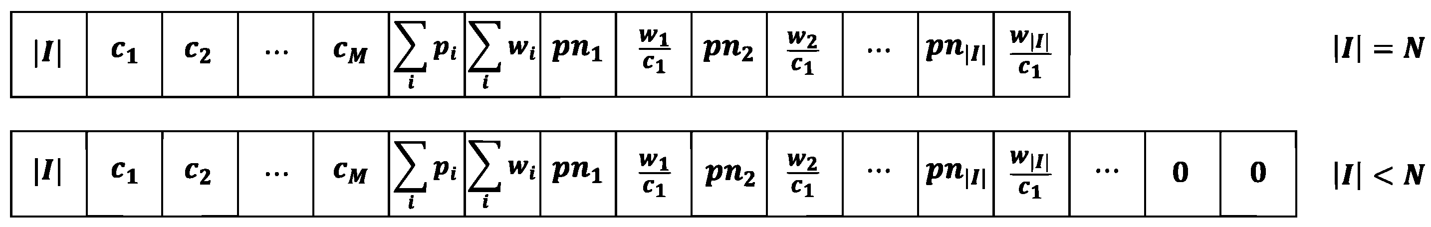
State: The proposed state has profit and weight information on at most N items to be selected, and the capacity information of all knapsacks. Figure 1 shows the proposed states of MKP. Let $\left|I\right|$ denote the number of items to be selected. Then, it indicates the number of problems for the agent to solve by selecting a single item at each time. Let $c_j$ denote the j-th largest capacity in the state. Each of the knapsack problems has a different target number, which is the number of not-fully-occupied knapsacks that can take more items. Because the target number of the knapsack is single, Afshar et al. [11] use one capacity field, whereas our method can use one or more capacity fields because we target not only a single knapsack but also multiple knapsacks. In Figure 1, it is assumed M is equal to the number of the knapsack. There are M capacity fields, which correspond to $c_1$, $c_2$, $c_3$, ⋯, $c_M$ and are sorted in descending order of the capacity size. At the first, $c_1$ with the largest size of the capacity is located, at the second, $c_2$ with the second largest size of the capacity is located, and at the last, $c_M$ with the smallest size of capacity is located. In Figure 1, ${\sum }_i{p}_i$ and ${\sum }_i{w}_i$ are the summed profit of items and the summed weight of items, respectively. In the following, profits and weights information on the items are listed. Here, $p{n}_i$ is a normalized $p_i$ as shown in (4).

$$p{n}_i=\frac{p_i}{p_{max}},$$

(4)

where $p_i$ is divided by $p_{max}$, which is the maximum size of the given profits. The pairs of $p{n}_i$ and $w_i/c_1$ are listed in descending order of $\frac{p_i}{w_i}$ value ($i\in I$). In the fields of each item, $p{n}_i$ is located at the first, and $\frac{w_i}{c_1}$ is located at the second. As a result, $p{n}_1$ is located at the first, and $\frac{w_1}{c_1}$ is located at the second. On the third, $p{n}_2$ is located, and on the fourth $\frac{w_2}{c_1}$ is located. The left items are listed in the same way. If an item is selected for a certain knapsack or discarded, the state does not have the item’s information anymore. The left $(N-|I\left|\right)\times 2$ fields have zero values.

Action: In action space, there are N actions $A=\{1,...,N\}$. An action $a\in A$ implies that the a-th item in item set I is selected and is put into the knapsack that has a maximum capacity $c_1$. Note that the size of action space is fixed to N regardless of the number of knapsacks.

Reward functions: If the agent’s action successfully allocates the item to the knapsack, the environment returns a positive reward. When the item’s weight exceeds the capacity of the target knapsack, a negative reward is given. When the chosen action is greater than the number of remaining items and an already chosen item is chosen, a fatal negative reward is given compared to the previous negative case. The proposed reward value is given by

$$r_t=\left\{\begin{array}{cc}p{n}_i,\hfill & w_i\le c_j\hfill \\ -\eta ,\hfill & w_i>c_j\hfill \\ -\xi ,\hfill & a\ge \left|I\right|.\hfill \end{array}\right.$$

(5)

Our reward value is different from that in [11], which is given by

$$\widehat{r_t}=\left\{\begin{array}{cc}\frac{p_i}{w_i·c},\hfill & w_i\le c\hfill \\ -\frac{w_i}{c},\hfill & w_i>c\hfill \\ -c,\hfill & a\ge \left|I\right|.\hfill \end{array}\right.$$

(6)

In the first case, the reward is set to $p{n}_i$ without considering the effect of weight and capacity so that the objective is closer to the MKP’s objective function in (1). In the second reward case of -$\eta$, we remove the effect of the weight of the violated item on the reward because the only thing the agent needs to know is whether the weight exceeds the capacity or not. Similarly, in the last reward case of -$\xi$, the only important thing is whether the item has already been chosen or not. Hence, we remove the effect of the capacity size compared with that in [11].

3.3. DRL Approaches

Our purpose is to obtain the maximum summed profits within reasonable computational steps according to the reward functions. To accomplish our purpose, A3C [20,32] is used for our policy model. The proposed policy model is parameterized by $\theta$ for the policy and ${\theta }_v$ for the critic’s value function as done in [33]. Using ${\mathbb{E}}_{{\pi }_{\theta }}\left[{\nabla }_{\theta }\right|log{\pi }_{\theta }(s,a)V_{{\theta }_v}\left(s_t\right)]=0$, the expected return value in (2) and its derivative in (3) can be replaced with the expected advantage value and its derivative, respectively, as follows:

$$J\left(\theta \right)={\mathbb{E}}_{{\pi }_{\theta }}\left[A^{{\pi }_{\theta }}(s,a)\right]$$

(7)

$${\nabla }_{\theta }\left(J\right)={\mathbb{E}}_{{\pi }_{\theta }}\left[{\nabla }_{\theta }\right|log{\pi }_{\theta }(s,a)A^{{\pi }_{\theta }}(s,a)],$$

(8)

where $A^{{\pi }_{\theta }}(s,a)$ denotes advantage got by ${\pi }_{\theta }$. The advantage value is obtained by subtracting baseline value from the return value and is given by

$$A_t^{{\pi }_{\theta }}=r_{t+1}+\gamma V_{{\theta }_v}\left(s_{t+1}\right)-V_{{\theta }_v}\left(s_t\right).$$

(9)

Note that the above equation in (9) gives one step advantage function.

According to the update interval, we use critic’s estimated value functions for getting each advantage value. Because $A_t^{{\pi }_{\theta }}$ in (9) is same to one step temporal difference (TD) error, it can be represented as $\delta \left({\theta }_v^t\right)$. As a result, the expected value of $A^{{\pi }_{\theta }}(s,a)$ and expected value of $\delta \left({\theta }_v^t\right)$ are the same.

$${\mathbb{E}}_{{\pi }_{\theta }}\left[\delta \left({\theta }_v^t\right)\right]={\mathbb{E}}_{{\pi }_{\theta }}\left[A_t^{{\pi }_{\theta }}\right].$$

(10)

Loss functions are composed of value loss and policy loss. Value loss is a mean squared error of TDs, and policy loss is negative $log{\pi }_{\theta }\left(a_t\right|s_t)$ times constant TD error.

$$\mathrm{Loss}=\frac{1}{T}\sum _{t=0}^{T-1}{\left(\delta \left({\theta }_v^t\right)\right)}^2+(-log{\pi }_{\theta }\left(a_t\right|s_t)\left[\delta \left({\theta }_v^t\right)\right]).$$

(11)

Under the assumption that the update interval is T, $\theta$ is updated according to the loss function as shown in (11).

3.4. Proposed Algorithm

We use multiple actor-learners to exploit different explorations in parallel to maximize diversity rather than one actor-learner model. It reduces correlation in accordance with a time in a single learner’s update method. Furthermore, it can shorten the training time and make the on-policy method more stable [32].

Algorithm 1 shows the asynchronous training process. Multiple subprocesses with their local model copy the global model’s parameters to the local model before starting the following episode. After the end of each episode and learning process of Algorithm 2, the global model’s parameters are updated to the trained local model’s.

Algorithm 1 Asynchronous process

Input: N (the number of items), M (the number of knapsacks), $AL$ (the number of actor-learners) Output: Trained global model 1: Initialize a policy network ${\pi }_{\theta }\left(a_t\right|s_t)$ with parameters $\theta$ for global model and value function $V_{{\theta }_v}\left(s_t\right)$ with parameters ${\theta }_v$ 2: $Proces{s}_{max}=AL,i=0$ 3: while$i<Proces{s}_{max}$do 4:       Process i starts training process 5: end while

Algorithm 2 runs on the process with the actor-critic model. Input is K problem instances with N items. The total iteration of training episodes is K × R in line 1. In every iteration, episode i uses the e-th instance in the range between 0 and ($K-1$) in line 3. The number of initial items at each episode is a random integer number between 1 and N. The initial capacity of each knapsack is a random integer value between the minimum weight of the item sets and maximum capacity C. While there is at least one candidate item, each step of an episode iterates. The episode is over when capacities are not sufficient, or overall items are chosen (selected or discarded), i.e., $\left|I\right|=0$. An action is always chosen from the range between 1 and N. In line 12, the agent does an action according to the policy ${\pi }_{\theta }\left(a_t\right|s_t)$. If the chosen item is not selected or discarded yet, and its weight is less than or equal to $c_1$, then the item is selected for the knapsack. As a result, capacity $c_1$ changes to current capacity minus the weight of the selected item according to action a (line 15). The item is classified as selected one and is excluded from the item set I (line 16 and 18). $ai$ denotes an index of the initial item set. Subsequently, Algorithm 3 is called and constitutes the capacity features of the next state. The output of Algorithm 2 is decision variables of items for each instance in K.

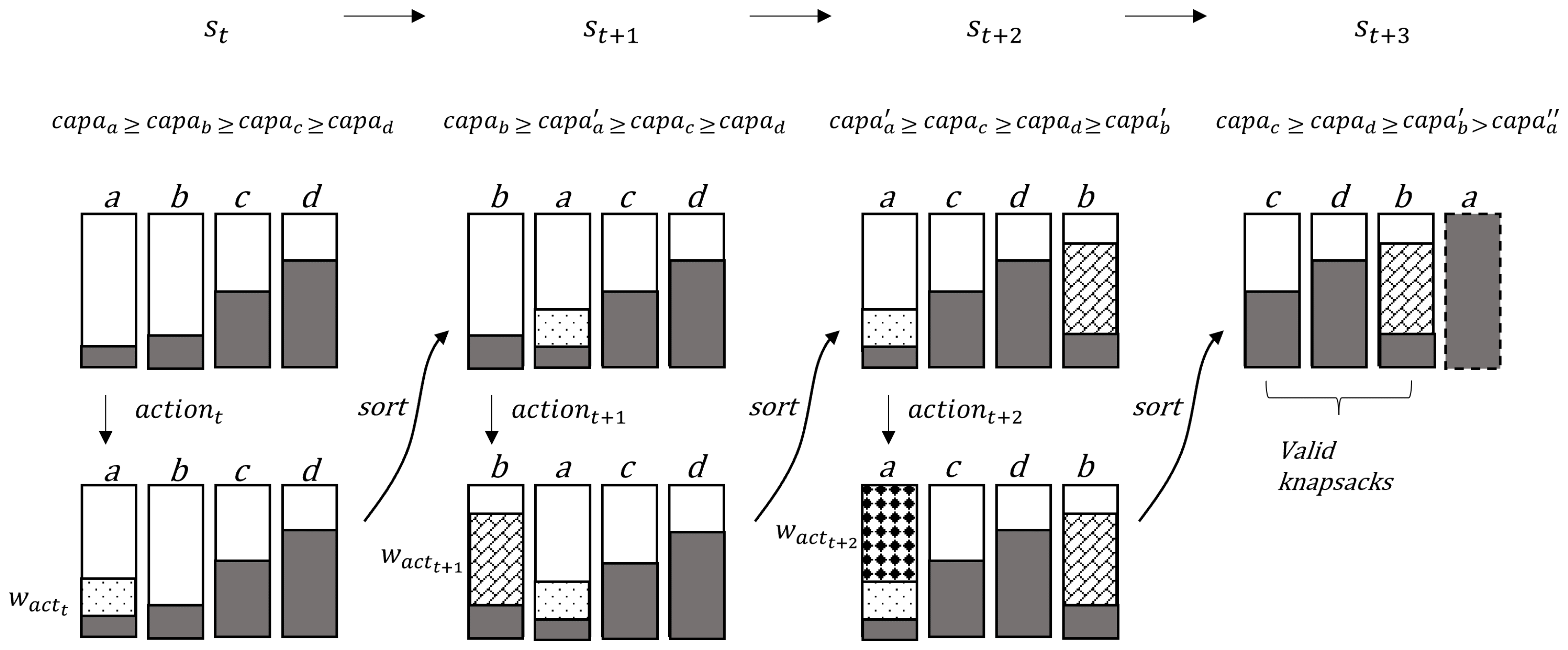
Algorithm 3 is a greedy sort algorithm for the very next state following action in Algorithm 2. This sorts the capacities in the descending order, and it only deals with capacities that are larger than zero. Therefore, the process creates new sorted capacities $c_1$, ⋯, $c_V$ for $V\le M$. Figure 2 shows an example of the sorting process. In state $s_t$, knapsacks are sorted as a, b, c, d according to the initial capacities. The capacities are denoted by $cap{a}_a$, $cap{a}_b$, $cap{a}_c$, and $cap{a}_d$. When an item corresponding to the $actio{n}_t$ is selected and the weight constraint condition is satisfied, $cap{a}_a$ changes from the existing capacity to a value reduced by the weight of the item. Assume that the currently changed capacity of knapsack a is smaller than $cap{a}_b$ and larger than $cap{a}_c$ and $cap{a}_d$. At this point, the order of the knapsacks are sorted so that the subsequent state $s_{t+1}$ would contain the knapsacks’ current capacities that are $c_1=cap{a}_b$, $c_2=cap{a}_a^{{}^{\prime }}$, $c_3=cap{a}_c$, and $c_4=cap{a}_d$. For the following action in state $s_{t+1}$, the capacity of b changes, and knapsacks for $c_j$ are sorted again. When $cap{a}_a^{{}^{\prime \prime }}$ becomes zero in $s_{t+2}$, knapsack a becomes invalid. Then, the sorting process excludes the knapsack and sorts valid knapsacks whose capacities are larger than zero.

Algorithm 2 Training process

Input: K problem instances with N items and R repeat number, N (the number of items), M (the number of knapsacks), C (max capacity) Output: Trained model, solutions of the K instances 1: $Trainin{g}_{max}=K\times R,i=0$ 2: while$i<Trainin{g}_{max}$do      3:       e = i mod K, t = 0 4:       $d=$ random integer number $1\sim N$ 5:       $I=\{1,\cdots ,d\}$ 6:       $c_j=$ random integer number $min(w_n,n\in I)\sim C$ 7:       Sort items indicating I according to the profit over weight 8:       Call Algorithm 3 for greedy sorting capacities 9:       while $min(w_n,n\in I)\le c_1$ do 10:           $u=0$ 11:           while $u<update$ $interval$ do 12:                  Do action a according to the policy ${\pi }_{\theta }\left(a_t\right|s_t)$ 13:                  if $a<\left|I\right|$ then 14:                      if $w_a\le c_1$ then 15:                          $c_1\leftarrow c_1-w_a$ 16:                          $x_{ai}\leftarrow 1$ 17:                    end if 18:                    $I\leftarrow (I\setminus \{a\left\}\right)$ 19:              end if 20:              Call Algorithm 3 21:              $u\leftarrow u+1$ 22:              $t\leftarrow t+1$ 23:         end while 24:         Update global model’s $\theta$ and ${\theta }_v$ using (11) 25:         Copy global model to local model 26:      end while 27:      $i\leftarrow i+1$ 28: end while

Algorithm 3 Greedy sort

Input: Capacities and indices of knapsacks indicating $c_1,\cdots ,c_V$ Output: Sorted information of knapsacks indicating $c_1,\cdots ,c_V$ 1: Sort capacities of knapsacks indicating $c_1,\cdots ,c_V$ 2: j = 1 3: while$j\le V$do 4:       $c_j\leftarrow$ capacity of a knapsack which has the j-th largest capacity 5:       $j\leftarrow j+1$ 6: end while

3.5. Constructed Neural Networks

Our parameterized policy model is DNN based model. The DNN model is made up of one convolution layer with two kernels and two strides, one fully connected layer with 512 nodes, and one output layer for each actor and critic. The fully connected layer’s activation function is Rectified Linear Unit (ReLU), and the actor’s output layer’s activation function is a sigmoid function.

4. Performance Evaluation

The proposed algorithm is programmed using Pytorch. For training the A3C-based DNN model, we use the discount factor $\gamma$ near to 1 and a learning rate of 0.0001. The parameters of the model are initialized as random uniform values within $[-0.08,0.08]$. There are three types of problem instances for training the proposed model: random instances (RI), linear instances (LI), and quadratic instances (QI). Random instances have uniformly random integer values in the range of $[1,10]$ for both profit and weight. Linear instances have the same weight as RI, and profit of them has weight plus random float value in $(0,1)$. Quadratic instances have the same weight as RI, and profit of them has $weight\times (10-weight)+1$. In the problem instances, knapsack has the same capacity in $10,20,40,80,100$. The number of items is 50, and the number of knapsacks is $1,3,5$. To deal with diversified problems, we prepare various models, and each model solves problems of its type. Each model has one type of item set (one of RI, LI, QI), a fixed number of knapsacks, (one of 1, 3, 5), and a fixed maximum capacity C (one of 10, 20, 40, 80, 100). In the case of 5 knapsacks, there are three types of capacity (10, 20, 40) because more than 40 is sufficient to select all items. 1000 data sets are used for each problem instance, and the model’s parameters are updated each five steps, with the process repeated at least 40 times. Every test result is executed on a workstation equipped with an AMD Ryzen 9 5900 X 12-Core Processor 3.70 GHz and 32 GB RAM.

The comparable methods for the test are as follows.

• Greedy algorithm: We use a simple greedy algorithm that finds an item that has maximized profit divided by weight ratio and tries assigning the item to a knapsack with maximized capacity.
• Random solution: We repeat randomly generating solution of each data 1000 times and then select a solution that has a maximum profit ratio.
• Gurobi optimizer: We use a mathematical optimization tool Gurobi for optimized solutions.

4.1. Training Process

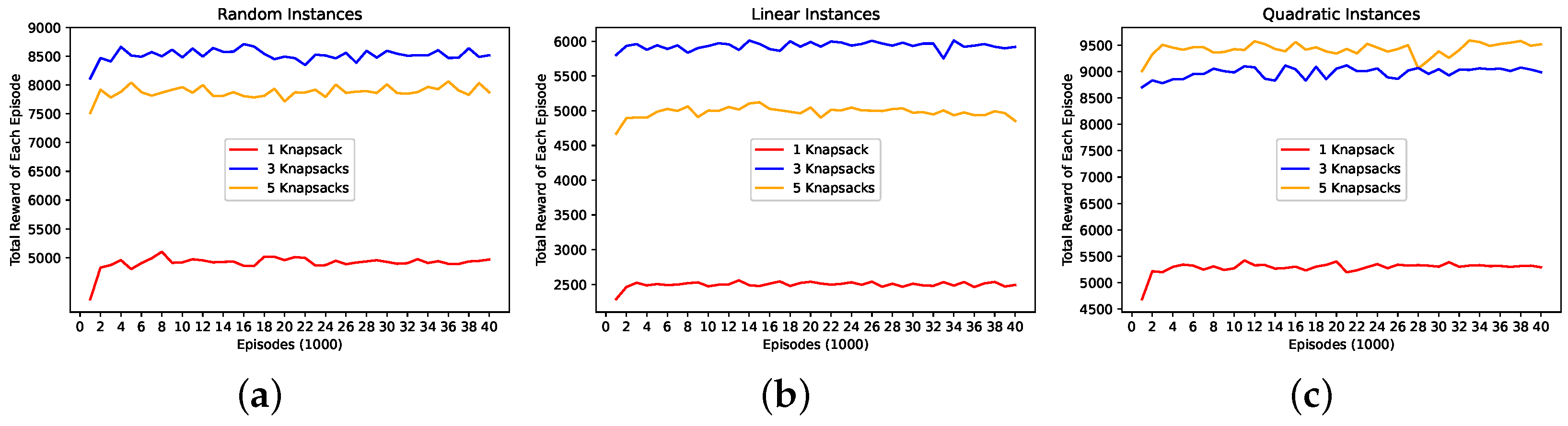
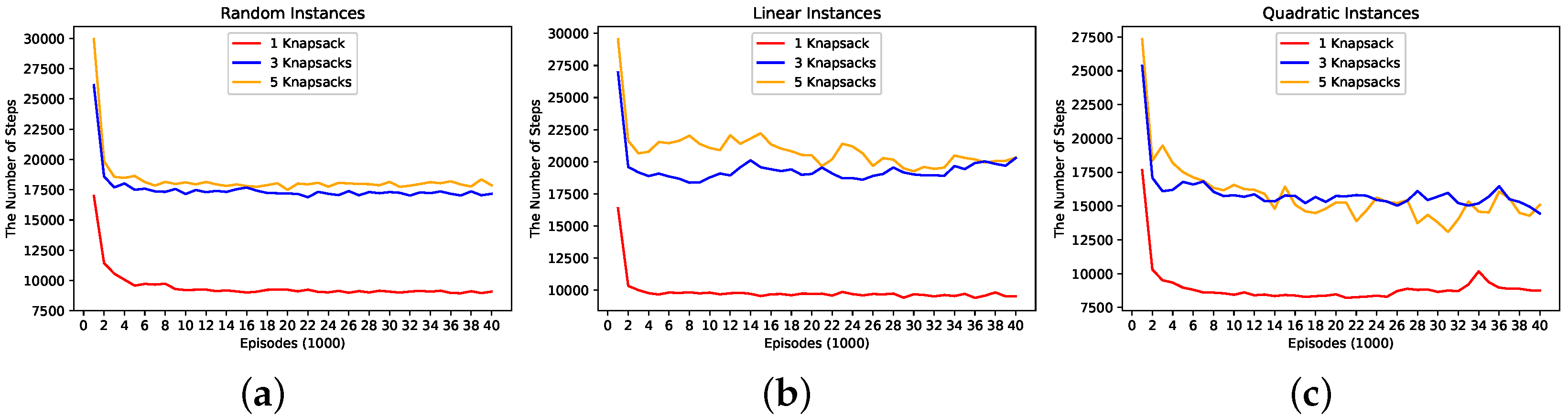
During training the DNN model, we summed a reward at each step in each episode and counted the number of steps to end each episode. Figure 3 and Figure 4 show the reward and the number of steps, respectively, according to the episode in the first 40,000 episodes. The x-axis in both figures represents a unit composed of consecutive 1000 episodes.

Figure 3 represents accumulated rewards after each unit of 1000 episodes proceeded. All three instances show that the accumulated reward during the second unit has a greater value than the reward accumulated during the first unit. Subsequently, oscillation occurs mainly caused by randomly given number of items and size of capacities in each episode. When the emergence of oscillation is considered, it is observed that the accumulated rewards converge to certain values. In such a way, for RI, LI, and QI, respectively, rewards converge to 8000, 5000, and 8500 in three knapsacks, and converge to 8500, 6000, and 9000 in 5 knapsacks, respectively.

Figure 4 represents accumulated number of steps during proceeding each unit of episodes. In Figure 4, it is observed that all three instances get through an enormous number of steps in the initial 1000 episodes. However, in the second 1000 episodes, they get through much less number of steps. In one knapsack, the number of steps for all instances converges to near 10,000. In three knapsacks, each number of steps converges to 17,500 for RI, 20,000 for LI, and values between 15,000 and 17,500 for QI. In five knapsacks, it converges to values between 17,500 and 20,000 for RI, 20,000 for LI, and values between 15,000 and 17,500 for QI.

4.2. Result of Solutions

In Section 4.1, we observed the trained models get better performance in terms of reward and number of steps. In this section, we will verify the performance of the trained models applied to unseen problems. The trained models and baseline methods solved 1000 problems per problem type. The types of problems are discussed in the first paragraph of Section 4. We calculated the average value based on the profits of the selected items in the solutions.

Table 1. Profit ratio of selected items for RI set.

M	N	Capacity	Random	Greedy	Proposed	Optimal
1	50	10	0.1507	0.1727	0.1727	0.1743
		20	0.2064	0.2652	0.2652	0.2672
		40	0.3002	0.3960	0.3958	0.3979
		80	0.4638	0.5853	0.5853	0.5873
		100	0.5354	0.6553	0.6551	0.6573
3	50	10	0.2786	0.3230	0.3256	0.3376
		20	0.4016	0.4855	0.4876	0.4995
		40	0.6138	0.7165	0.7166	0.7293
		80	0.9285	0.9678	0.9678	0.9738
		100	0.9952	0.9985	0.9985	0.9993
5	50	10	0.3665	0.4235	0.4268	0.4530
		20	0.5449	0.6323	0.6323	0.6609
		40	0.8239	0.9029	0.9030	0.9218

,

Table 2. Profit ratio of selected items for LI set.

M	N	Capacity	Random	Greedy	Proposed	Optimal
1	50	10	0.0467	0.0483	0.0483	0.0488
		20	0.0848	0.0893	0.0893	0.0901
		40	0.1587	0.1664	0.1664	0.1675
		80	0.3060	0.3153	0.3156	0.3170
		100	0.3798	0.3893	0.3894	0.3911
3	50	10	0.1238	0.1244	0.1263	0.1299
		20	0.2347	0.2377	0.2398	0.2442
		40	0.4522	0.4555	0.4581	0.4638
		80	0.8720	0.8642	0.8665	0.8830
		100	0.9914	0.9917	0.9929	0.9964
5	50	10	0.1956	0.1920	0.1920	0.2061
		20	0.3776	0.3751	0.3784	0.3920
		40	0.7240	0.7191	0.7208	0.7438

and

Table 3. Profit ratio of selected items for QI set.

M	N	Capacity	Random	Greedy	Proposed	Optimal
1	50	10	0.1010	0.1009	0.1046	0.1049
		20	0.1733	0.1888	0.1934	0.1951
		40	0.2847	0.3393	0.3436	0.3467
		80	0.4679	0.5826	0.5856	0.5879
		100	0.5450	0.6724	0.6749	0.6767
3	50	10	0.2496	0.2502	0.2634	0.2755
		20	0.3977	0.4463	0.4635	0.4760
		40	0.6314	0.7353	0.7351	0.7606
		80	0.9426	0.9869	0.9866	0.9911
		100	0.9970	0.9995	0.9995	0.9998
5	50	10	0.3574	0.3693	0.3693	0.4142
		20	0.5630	0.6284	0.6507	0.6819
		40	0.8478	0.9308	0.9355	0.9550

show the profit of selected items divided by the profit of total items. The optimal result of each instance represents the maximum feasible profit ratio in each knapsack and capacity.

Table 4. The closeness to the optimal solution in RI set.

M	N	Capacity	Random	Greedy	Proposed	Optimal
1	50	10	86.46	99.10	99.10	-
		20	77.24	99.28	99.28	-
		40	75.46	99.52	99.51	-
		80	79.01	99.66	99.66	-
		100	81.49	99.69	99.70	-
		Average	79.93	99.45	99.45	-
3	50	10	82.56	95.70	96.44	-
		20	80.44	97.21	97.62	-
		40	84.21	98.25	98.25	-
		80	95.34	99.38	99.38	-
		100	99.59	99.92	99.92	-
		Average	88.43	98.09	98.32	-
5	50	10	80.93	93.49	94.21	-
		20	82.49	95.68	95.68	-
		40	89.39	97.94	97.95	-
		Average	84.27	95.70	95.95	-
Average			84.32	98.06	98.21	-

,

Table 5. The closeness to the optimal solution in LI set.

M	N	Capacity	Random	Greedy	Proposed	Optimal
1	50	10	95.59	98.76	98.74	-
		20	94.08	99.11	99.11	-
		40	94.75	99.32	99.34	-
		80	96.54	99.46	99.56	-
		100	97.12	99.52	99.54	-
		Average	95.62	99.23	99.26	-
3	50	10	95.34	95.74	97.26	-
		20	96.12	97.30	98.18	-
		40	97.50	98.21	98.78	-
		80	98.76	97.88	98.13	-
		100	99.46	99.48	99.61	-
		Average	97.44	97.72	98.39	-
5	50	10	94.92	93.10	93.10	-
		20	96.33	95.68	96.52	-
		40	97.35	96.69	96.91	-
		Average	96.20	95.16	95.51	-
Average			96.45	97.71	98.06	-

and

Table 6. The closeness to the optimal solution in QI set.

M	N	Capacity	Random	Greedy	Proposed	Optimal
1	50	10	96.22	96.12	99.67	-
		20	88.83	96.71	99.11	-
		40	82.24	97.90	99.13	-
		80	79.71	99.10	99.61	-
		100	80.67	99.35	99.73	-
		Average	85.53	97.84	99.45	-
3	50	10	90.57	90.82	95.61	-
		20	83.62	93.75	97.38	-
		40	83.08	96.67	96.64	-
		80	95.13	99.57	99.54	-
		100	99.73	99.98	99.98	-
		Average	90.43	96.16	97.83	-
5	50	10	86.32	89.20	89.20	-
		20	82.63	92.16	95.46	-
		40	88.80	97.45	97.95	-
		Average	85.92	92.93	94.20	-
Average			87.51	96.06	97.61	-

show the percentage of profit derived from each algorithm over the profit of the optimal solution. The percentage of each field represents how close the derived solution is to the optimal solution.

Table 7. Profit of selected items in RI set.

M	N	Capacity	Random	Greedy	Proposed	Optimal
1	50	10	41.292	47.326	47.326	47.758
		20	56.822	73.034	73.034	73.566
		40	82.118	108.303	108.293	108.825
		80	127.443	160.748	160.748	161.3
		100	147.755	180.763	180.765	181.318
		Average	91.086	114.0348	114.0332	114.5534
3	50	10	76.192	88.319	89.002	92.287
		20	110.333	133.321	133.89	137.154
		40	168.359	196.425	196.437	199.933
		80	255.865	266.714	266.714	268.37
		100	272.998	273.911	273.914	274.129
		Average	176.7494	191.738	191.9914	194.3746
5	50	10	100.253	115.813	116.701	123.873
		20	150.122	174.13	174.13	181.996
		40	226.462	248.135	248.157	253.353
		Average	158.9457	179.3593	179.6627	186.4073
Average			139.693	158.996	159.162	161.836

,

Table 8. Profit of selected items in LI set.

M	N	Capacity	Random	Greedy	Proposed	Optimal
1	50	10	13.893	14.353	14.350	14.533
		20	25.248	26.600	26.600	26.838
		40	47.588	49.880	49.891	50.223
		80	91.610	94.383	94.482	94.896
		100	113.521	116.333	116.355	116.891
		Average	58.372	60.310	60.336	60.676
3	50	10	36.809	36.963	37.552	38.609
		20	69.819	70.676	71.314	72.634
		40	134.866	135.845	136.632	138.321
		80	260.752	258.425	259.095	264.028
		100	297.773	297.832	298.217	299.392
		Average	160.004	159.948	160.562	162.597
5	50	10	58.286	57.168	57.168	61.405
		20	112.250	111.501	112.476	116.531
		40	216.931	215.463	215.970	222.845
		Average	129.156	128.044	128.538	133.594
Average			113.796	114.263	114.623	116.704

and

Table 9. Profit of selected items in QI set.

M	N	Capacity	Random	Greedy	Proposed	Optimal
1	50	10	87.785	87.701	90.937	91.238
		20	150.314	163.655	167.717	169.217
		40	248.873	296.239	299.961	302.608
		80	409.533	509.123	511.738	513.757
		100	476.957	587.385	589.609	591.216
		Average	274.692	328.821	331.992	333.607
3	50	10	216.993	217.575	229.067	239.574
		20	347.519	389.616	404.681	415.581
		40	549.914	639.802	639.619	661.874
		80	825.29	863.778	863.491	867.508
		100	873.759	875.893	875.901	876.105
		Average	562.695	597.333	602.552	612.128
5	50	10	311.933	322.349	322.349	361.385
		20	489.821	546.285	565.848	592.788
		40	741.96	814.227	818.424	835.539
		Average	514.571	560.954	568.874	596.571
Average			440.819	485.664	490.719	501.415

show the total profit of the selected items.

Table 10. Average profit of selected items per capacity in RI.

N	Capacity	Random	Greedy	Proposed	Optimal
50	10	72.579	83.819	84.343	87.973
	20	105.759	126.828	127.018	130.905
	40	158.980	184.288	184.296	187.370
	80	191.654	213.731	213.731	214.835
	100	210.377	227.337	227.340	227.724

,

Table 11. Average profit of selected items per capacity in LI.

N	Capacity	Random	Greedy	Proposed	Optimal
50	10	36.329	36.161	36.357	38.182
	20	69.106	69.592	70.130	72.001
	40	133.128	133.729	134.164	137.130
	80	176.181	176.404	176.788	179.462
	100	205.647	207.083	207.286	208.142

and

Table 12. Average profit of selected items per capacity in QI.

N	Capacity	Random	Greedy	Proposed	Optimal
50	10	205.570	209.208	214.118	230.732
	20	329.218	366.519	379.415	392.529
	40	513.582	583.423	586.001	600.007
	80	617.412	686.451	687.615	690.633
	100	675.358	731.639	732.755	733.661

represent the average profits of the selected items per capacity. Each field of them is an average value of the aggregate profit of the selected items in all knapsacks for a given capacity.

4.2.1. Random Instances

The optimal result in Table 1 shows 0.1743∼0.6573 profit ratio of selected items in a single knapsack. It means the maximized solution in a single knapsack can have a profit ratio up to 0.1743∼0.6573. Furthermore, as shown in Table 4, 99% of the closeness appears in both the proposed algorithm and the greedy algorithm in all sizes of capacity in single knapsacks. In Table 7, it is observed that the proposed algorithm’s average profit of a single knapsack differs by only 0.001 from the greedy algorithm’s. In the 3-knapsack case, in 10 and 20 capacity, the proposed algorithm is superior to the random solution and the greedy algorithm. In the 5-knapsack case, in 10 capacity, the proposed algorithm showed an outstanding result than the greedy algorithm. The proposed algorithm earns a profit of 166 more than the greedy algorithm when solving 1000 problems. In terms of capacity, as shown in Table 10, the average profit of the proposed algorithm has equally highest value or the highest value in the overall capacity.

4.2.2. Linear Instances

In a single knapsack, the profit of the selected item can be up to 0.0488∼0.3911 as shown in Table 2. In terms of closeness to the optimal solution, as the size of capacity becomes larger, the closeness also becomes larger. The proposed algorithm has 98.7% in 10 capacity and 99.5% in 100 capacity. The proposed algorithm outperforms other algorithms in 40, 80, 100 capacity. In the three-knapsack case, except for capacity 80, the proposed algorithm shows outstanding results. Except for capacity 20, the proposed algorithm and the greedy method fall short of the random solution in the five-knapsack case. In capacity 20, the proposed algorithm outperforms the other two algorithms. The average profit of the proposed algorithm has the highest value in the overall capacity as shown in Table 11.

4.2.3. Quadratic Instances

In a single knapsack, the profit ratio of selected items can be up to 0.1049∼0.6767 as shown in Table 3. In terms of closeness to the optimal solution, the proposed algorithm’s result shows 99% in overall capacity, and it outperforms other algorithms. The average profit of the proposed algorithm gets 3.171, 5.219, 7.92 more profit than the greedy algorithms in a single knapsack case, three-knapsack case, and in the five-knapsack case, respectively. When solving 1000 problems, the proposed algorithm earns a profit of 5055 more than the greedy algorithm. In terms of capacity as shown in Table 12, the average profit of the proposed algorithm has the highest value in the overall capacity.

4.3. Computational Time

Table 13. Computation time (seconds) in RI.

M	N	Capacity	Random	Greedy	Proposed	Optimal
		10	42.548	0.094	3.121	10.875
		20	43.171	0.109	4.438	12.043
1	50	40	44.491	0.109	6.256	14.060
		80	47.343	0.125	8.337	16.530
		100	48.260	0.125	8.936	17.406
		10	43.115	0.172	6.846	20.756
		20	45.137	0.172	10.267	21.039
3	50	40	48.254	0.172	11.508	25.326
		80	51.607	0.169	14.087	29.009
		100	52.505	0.172	15.318	27.187
		10	44.645	0.203	13.324	24.618
5	50	20	47.890	0.188	11.789	29.347
		40	50.471	0.188	13.796	32.295
Average			46.880	0.154	9.848	21.576

,

Table 14. Computation time (seconds) in LI.

M	N	Capacity	Random	Greedy	Proposed	Optimal
		10	52.549	0.109	3.396	8.696
		20	53.002	0.141	4.910	9.176
1	50	40	44.479	0.125	6.915	10.281
		80	47.641	0.125	9.117	14.083
		100	48.550	0.109	10.374	14.842
		10	51.214	0.188	9.360	19.139
		20	45.742	0.172	12.804	27.927
3	50	40	47.496	0.172	13.280	32.529
		80	51.170	0.172	14.493	42.591
		100	51.073	0.175	15.415	28.046
		10	44.677	0.203	11.613	33.515
5	50	20	47.423	0.187	14.379	40.987
		40	51.020	0.172	19.191	52.013
Average			48.926	0.158	11.173	25.679

and

Table 15. Computation time (seconds) in QI.

M	N	Capacity	Random	Greedy	Proposed	Optimal
		10	42.438	0.109	3.222	8.800
		20	43.232	0.109	3.719	9.566
1	50	40	44.211	0.125	9.369	10.872
		80	46.144	0.125	8.274	12.444
		100	47.784	0.125	12.986	12.904
		10	43.792	0.172	6.445	16.455
		20	45.239	0.171	9.554	20.504
3	50	40	48.214	0.172	9.661	24.433
		80	51.516	0.172	14.420	22.745
		100	50.897	0.172	15.891	21.201
		10	45.092	0.199	5.801	24.654
5	50	20	47.295	0.203	9.754	46.842
		40	49.980	0.183	13.736	33.331
Average			46.603	0.157	9.449	20.366

shows computation time solving 1000 test problems in RI, LI, and QI, respectively. The proposed method’s results are the second-fastest in the overall tables, trailing only the greedy method. Both the optimal and random solutions fall short of the previous two methods. The proposed algorithm and optimal solution are heavily influenced by the capacity of each knapsack.

4.4. Overall Evaluation

The greedy algorithm is very fast, but its performance was not the best in many cases of the experiments. The greedy algorithm, in particular, would be vulnerable when it encountered instances where profit and weight are correlated, such as LI. The proposed method can provide a more robust solution because it produced excellent results in a variety of situations, including the correlation between profit and weight.

5. Conclusions

In this paper, to solve MKP efficiently, we proposed a DRL-based solution. The proposed method trains the neural model by using A3C algorithm. The experiments show the proposed method achieves higher performance compared to the greedy algorithm and random solution. The results in random, linear, and quadratic instances demonstrated that the proposed algorithm is robust. Consequently, we verified that the proposed method is appropriate for solving real-world MKPs with varying profit, weight, and capacity.

References

- Assi, M.; Haraty, R.A. A Survey of the Knapsack Problem. In Proceedings of the International Arab Conference on Information Technology (ACIT), Werdanye, Lebanon, 28–30 November 2018; pp. 1–6. [Google Scholar] [CrossRef]
- Lahyani, R.; Chebil, K.; Khemakhem, M.; Coelho, L.C. Matheuristics for solving the multiple knapsack problem with setup. Comput. Ind. Eng. 2019, 129, 76–89. [Google Scholar] [CrossRef]
- Kumaraguruparan, N.; Sivaramakrishnan, H.; Sapatnekar, S.S. Residential task scheduling under dynamic pricing using the multiple knapsack method. In Proceedings of the IEEE PES Innovative Smart Grid Technologies (ISGT), Washington, DC, USA, 16–20 January 2012; pp. 1–6. [Google Scholar]
- Ketykó, I.; Kecskés, L.; Nemes, C.; Farkas, L. Multi-user computation offloading as multiple knapsack problem for 5G mobile edge computing. In Proceedings of the European Conference on Networks and Communications (EuCNC), Athens, Greece, 27–30 June 2016; pp. 225–229. [Google Scholar]
- Cappanera, P.; Paganelli, F.; Paradiso, F. VNF placement for service chaining in a distributed cloud environment with multiple stakeholders. Comput. Commun. 2019, 133, 24–40. [Google Scholar] [CrossRef]
- Martello, S.; Toth, P. Knapsack Problems: Algorithms and Computer Implementations; John Wiley & Sons, Inc.: Hoboken, NJ, USA, 1990. [Google Scholar]
- Arulkumaran, K.; Deisenroth, M.P.; Brundage, M.; Bharath, A.A. Deep reinforcement learning: A brief survey. IEEE Signal Process. Mag. 2017, 34, 26–38. [Google Scholar] [CrossRef] [Green Version]
- Lillicrap, T.P.; Hunt, J.J.; Pritzel, A.; Heess, N.; Erez, T.; Tassa, Y.; Silver, D.; Wierstra, D. Continuous control with deep reinforcement learning. arXiv 2015, arXiv:1509.02971. [Google Scholar]
- Silver, D.; Huang, A.; Maddison, C.J.; Guez, A.; Sifre, L.; Van Den Driessche, G.; Schrittwieser, J.; Antonoglou, I.; Panneershelvam, V.; Lanctot, M.; et al. Mastering the game of Go with deep neural networks and tree search. Nature 2016, 529, 484–489. [Google Scholar] [CrossRef] [PubMed]
- Gu, S.; Hao, T. A pointer network based deep learning algorithm for 0–1 knapsack problem. In Proceedings of the International Conference on Advanced Computational Intelligence (ICACI), Xiamen, China, 29–31 March 2018; pp. 473–477. [Google Scholar]
- Afshar, R.R.; Zhang, Y.; Firat, M.; Kaymak, U. A State Aggregation Approach for Solving Knapsack Problem with Deep Reinforcement Learning. In Proceedings of the Asian Conference on Machine Learning (PMLR), Bangkok, Thailand, 18–20 November 2020; pp. 81–96. [Google Scholar]
- Dai, H.; Dai, B.; Song, L. Discriminative embeddings of latent variable models for structured data. In Proceedings of the 33rd International Conference on Machine Learning (PMLR), New York, NY, USA, 19–24 June 2016; pp. 2702–2711. [Google Scholar]
- Dai, H.; Khalil, E.B.; Zhang, Y.; Dilkina, B.; Song, L. Learning combinatorial optimization algorithms over graphs. arXiv 2017, arXiv:1704.01665. [Google Scholar]
- Kundu, O.; Dutta, S.; Kumar, S. Deep-pack: A vision-based 2d online bin packing algorithm with deep reinforcement learning. In Proceedings of the International Conference on Robot and Human Interactive Communication (RO-MAN), New Delhi, India, 14–18 October 2019; pp. 1–7. [Google Scholar]
- Zhang, Z.; Liu, H.; Zhou, M.; Wang, J. Solving Dynamic Traveling Salesman Problems With Deep Reinforcement Learning. IEEE Trans. Neural Netw. Learn. Syst. 2021. [Google Scholar] [CrossRef] [PubMed]
- Nazari, M.; Oroojlooy, A.; Snyder, L.; Takác, M. Reinforcement learning for solving the vehicle routing problem. In Proceedings of the 32nd International Conference on Advances in Neural Information Processing Systems, Montreal, QC, Canada, 3–8 December 2018. [Google Scholar]
- Chen, X.; Tian, Y. Learning to perform local rewriting for combinatorial optimization. In Proceedings of the 33nd International Conference on Advances in Neural Information Processing Systems, Vancouver, BC, Canada, 8–14 December 2019. [Google Scholar]
- Vinyals, O.; Fortunato, M.; Jaitly, N. Pointer networks. arXiv 2015, arXiv:1506.03134. [Google Scholar]
- Bello, I.; Pham, H.; Le, Q.V.; Norouzi, M.; Bengio, S. Neural combinatorial optimization with reinforcement learning. arXiv 2016, arXiv:1611.09940. [Google Scholar]
- Mnih, V.; Badia, A.P.; Mirza, M.; Graves, A.; Lillicrap, T.; Harley, T.; Silver, D.; Kavukcuoglu, K. Asynchronous methods for deep reinforcement learning. In Proceedings of the International Conference on Machine Learning (PMLR), New York, NY, USA, 19–24 June 2016; pp. 1928–1937. [Google Scholar]
- Pisinger, D. An exact algorithm for large multiple knapsack problems. Eur. J. Oper. Res. 1999, 114, 528–541. [Google Scholar] [CrossRef]
- Dell’Amico, M.; Delorme, M.; Iori, M.; Martello, S. Mathematical models and decomposition methods for the multiple knapsack problem. Eur. J. Oper. Res. 2019, 274, 886–899. [Google Scholar] [CrossRef]
- Srinivas, M.; Patnaik, L.M. Genetic algorithms: A survey. Computer 1994, 27, 17–26. [Google Scholar] [CrossRef]
- Khuri, S.; Bäck, T.; Heitkötter, J. The zero/one multiple knapsack problem and genetic algorithms. In Proceedings of the 1994 ACM Symposium on Applied Computing, Phoenix, AZ, USA, 6–8 March 1994; pp. 188–193. [Google Scholar]
- Falkenauer, E. A new representation and operators for genetic algorithms applied to grouping problems. Evol. Comput. 1994, 2, 123–144. [Google Scholar] [CrossRef]
- Fukunaga, A.S. A new grouping genetic algorithm for the multiple knapsack problem. In Proceedings of the 2008 IEEE Congress on Evolutionary Computation, Hong Kong, China, 1–6 June 2008; pp. 2225–2232. [Google Scholar]
- Han, K.H.; Kim, J.H. Quantum-inspired evolutionary algorithm for a class of combinatorial optimization. IEEE Trans. Evol. Comput. 2002, 6, 580–593. [Google Scholar] [CrossRef] [Green Version]
- Hu, H.; Zhang, X.; Yan, X.; Wang, L.; Xu, Y. Solving a new 3d bin packing problem with deep reinforcement learning method. arXiv 2017, arXiv:1708.05930. [Google Scholar]
- Rezoug, A.; Bader-El-Den, M.; Boughaci, D. Application of Supervised Machine Learning Methods on the Multidimensional Knapsack Problem. Neural Process. Lett. 2021, 1–20. [Google Scholar] [CrossRef]
- García, J.; Lalla Ruiz, E.; Voß, S.; Lopez Droguett, E. Enhancing a machine learning binarization framework by perturbation operators: Analysis on the multidimensional knapsack problem. Int. J. Mach. Learn. Cybern. 2020, 11, 1951–1970. [Google Scholar] [CrossRef]
- Laterre, A.; Fu, Y.; Jabri, M.K.; Cohen, A.S.; Kas, D.; Hajjar, K.; Dahl, T.S.; Kerkeni, A.; Beguir, K. Ranked reward: Enabling self-play reinforcement learning for combinatorial optimization. arXiv 2018, arXiv:1807.01672. [Google Scholar]
- Silver, D.; Lever, G.; Heess, N.; Degris, T.; Wierstra, D.; Riedmiller, M. Deterministic policy gradient algorithms. In Proceedings of the International Conference on Machine Learning (PMLR), Beijing, China, 21–26 June 2014; pp. 387–395. [Google Scholar]
- Silver, D. Lectures on Reinforcement Learning. 2015. Available online: https://www.davidsilver.uk/teaching/ (accessed on 11 March 2022).
Figure 1.
State of multiple knapsack problem.
Figure 2.
Capacities of knapsacks in each state.
Figure 3.
DRL training information of reward in episodes. (a) Reward of RI; (b) Reward of LI; (c) Reward of QI.
Figure 4.
DRL training information of step in episodes. (a) Step of RI; (b) Step of LI; (c) Step of QI.