A Study on Reversible Data Hiding Technique Based on Three-Dimensional Prediction-Error Histogram Modification and a Multilayer Perceptron

Abstract

In the past few years, with the development of information technology and the focus on information security, many studies have gradually been aimed at data hiding technology. The embedding and extraction algorithms are mainly used by the technology to hide the data that requires secret transmission into a multimedia carrier so that the data transmission cannot be realized to achieve secure communication. Among them, reversible data hiding (RDH) is a technology for the applications that demand the secret data extraction as well as the original carrier recovery without distortion, such as remote medical diagnosis or military secret transmission. In this work, we hypothesize that the RDH performance can be enhanced by a more accurate pixel value predictor. We propose a new RDH scheme of prediction-error expansion (PEE) based on a multilayer perceptron, which is an extensively used artificial neural network in plenty of applications. The scheme utilizes the correlation between image pixel values and their adjacent pixels to obtain a well-trained multilayer perceptron so that we are capable of achieving more accurate pixel prediction results. Our data mapping method based on the three-dimensional prediction-error histogram modification uses all eight octants in the three-dimensional space for secret data embedding. The experimental results of our RDH scheme show that the embedding capacity greatly increases and the image quality is still well maintained.

1. Introduction

1.1. Background

With the rapid development of information technology, the internet has been ubiquitous in the world. Thanks to the development of optical communication systems (see [1] for more discussions), people can easily communicate with each other and share multimedia messages, including texts, sound, images, videos, etc. Obviously, the internet provides much more impact on human society than any other medium, while at the same time, issues regarding information security have received considerable and critical attention.

Data hiding is an available technique to deal with secure communication so that the secure data is imperceptibly embedded without drawing attention [2]. The multimedia is used as a cover carrier to hide secret data which will be transmitted in the internet. Reversible data hiding (RDH) not only guarantees the safe transmission of data content but also recovers the hidden data as well as the cover images [3,4]. However, most of these RDH algorithms bring permanent distortions to the original carrier during the embedding process, and these distortions are unacceptable in certain applications [5]. In order to achieve information hiding and distortion-free recovery of the original carrier, distortion-free reversible data hiding is considered [4]. This technique enables the receiver to both extract the embedded data correctly and acquire the original carrier without distortion. Generally, RDH is a fragile hiding technology, which is different from digital watermarking. When implementing the RDH mothod, the distortion that occurs during the transmission of the carrier should be avoided. According to the embedding method, the existing image RDH algorithm can be divided into spatial domain, transform domain, and encryption domain RDH scheme [6]. In this paper, we focus on RDH of spatial domain. Its embedding and extraction frameworks are shown in Figure 1. In the embedding side, the sender embeds secret data into the cover image by a reversible embedding algorithm. In the extraction side, the receiver extracts the secret data embedded in the stego-image by a reversible extraction algorithm and achieves distortion-free recovery image exactly the same as the original image. The performance of RDH algorithm depends on two conflicting factors as trade-offs: the embedding distortion between the cover image and the stego-image and the embedding capacity (EC). For the former factor, PSNR (peak-to-noise-ratio) is widely used (refer to [7] for more discussion). A higher PSNR value means that the stego-image is more similar to the original one. For the latter factor, EC stands for the number of bits which can be embedded into the cover image. Therefore, we favor an RDH algorithm which brings higher EC and lower PSNR, while a trade-off of them is usually considered to fit specific applications [6].

1.2. Prediction-Error Expansion

In this subsection, we introduce the RDH paradigm we mainly follow: the prediction-error expansion (PEE) approach, which was first proposed by Thodi and Rodriguez [8]. PEE is a kind of histogram-shifting technique for which histograms of the feature elements (e.g., pixel values, errors between cover pixel values and their predicted values) are shifted to prepare vacant positions for embedding the secret bits. Since the most frequent feature elements determines the EC, and moreover, peaks of the prediction-error histograms usually center at zero, PEE has the advantage over the other histogram-shifting techniques in the spatial domain, especially for the cover image with flat pixel value histogram [9].

PEE can exploit spatial redundancy in the image. The correlation of local neighborhood of each pixel is taken into consideration. Following a certain order of scanning the original image, a predictor is used to make prediction of each pixel. Denote by $\widehat{x}$ the predicted value of a pixel x. The prediction-error of x is defined as $e_x=x-\widehat{x}$. One can expand the prediction-error $e_x$ to be $e_x^{*}=f(e_x,m)$ for some shifting operation f and a to-be-embedded bit $m\in \{0,1\}$. When the context is clear, we omit the parameter m in f to make formula concise. In the stego-image this pixel will be $\tilde{x}=\widehat{x}+e_x^{*}$. As illustrated in [5],

$$e_x^{*}=\left\{\begin{array}{cc}{e}_x+m,\hfill & \mathrm{if}{e}_x=0\hfill \\ e_x-m,\hfill & \mathrm{if}{e}_x=-1\hfill \\ e_x+1,\hfill & \mathrm{if}{e}_x>0\hfill \\ e_x-1,\hfill & \mathrm{if}{e}_x<-1\hfill \end{array}\right.,$$

where $m\in \{0,1\}$ is a to-be-embedded bit. At pixel x at which $e_x\in \{0,-1\}$, a secret bit is embedded, while for pixel x at which $e_x\notin \{0,-1\}$, the pixel value is shifted by 1 or $-1$. With prediction-errors at hand, the prediction-error histogram (PEH) can be created as $h\left(a\right)=|\{i:e_i=a\}|$ for each prediction-error a. Specifically, PEE can be implemented as histogram modification of the PEH, that is, expanding the bins of $-1$ and 0 and shifting the other bins to create space to ensure the reversibility. Such a paradigm has been extended to 2D-PEH (e.g., [10]), where the PEH is defined by $h_2(a,b)=|i:(e_{2i-1},e_{2i})=(a,b)|$, and also 3D-PEH (e.g., [5]), where the PEH is defined as $h_3(a,b,c)=|i:(e_{3i-2},e_{3i-1},e_{3i})=(a,b,c)|$. Here we have $f:{\mathbf{Z}}^3\mapsto \mathcal{P}\left({\mathbf{Z}}^3\right)$ to be a mapping which realizes RDH, where $\mathcal{P}\left(A\right)$ denotes the power set of a set A, such that $f\left(p\right)$ represents the set of marked prediction-errors for a prediction-error p (e.g., $p=(e_{3i-2},e_{3i-1},e_{3i})$ for some i). As long as $f\left(p\right)\ne \varnothing$ for any prediction-error p and $f\left(p\right)\cap f\left(q\right)=\varnothing$ for every two prediction-errors p and q, the reversibility of the mapping can be guaranteed. PEE has attracted considerable attention [5,8,9,10,11,12,13,14,15,16,17,18,19,20,21,22,23,24,25,26,27] since it can maintain low embedding distortion while at the same time provide sufficiently large payload in terms of high EC.

1.3. Our Contribution

As the illustrating example of PEE shows, EC depends on the prediction accuracy of the pixels. When PEE is applied, the data bits are embedded only when the prediction-error is $-1$ or 0. Hence, we have the following hypothesis.

Hypothesis 1.

As the prediction accuracy is improved, the performance of the PEE techniques for RDH is enhanced.

In this paper, we devote our efforts in validating this hypothesis. Specifically, we aim at improving the prediction accuracy in PEE using deep an artificial neural network (ANN), which has been developed rapidly and extensively studied in the past decade. We propose a novel method based on a multilayer perceptron (MLP), which is a well-known ANN consisting of multiple sequential fully connected layers and providing nonlinear mapping between input data and output data with nonlinear activation functions. Moreover, we consider eight octants in the three-dimensional space for embedding, which makes better use of space (c.f. [5] which considers only the first octant for the embedding). We conduct experiments by applying our proposed method on six test images, including Lena, Baboon, Boat, Peppers, Airplane (F-16), and House. The experimental results well support our hypothesis. The EC greatly increases and is 1.9–9.8 times of previous methods. On the other hand, the image quality is still well maintained in terms of low PSNR, which is competitive compared with previous work.

Remark 1.

Our MLP consists of layers of nodes. The nodes between consecutive layers are fully connected by weighted edges. Each node receives input from nodes on the previous layer and sends output by passing the aggregated input to a nonlinear activation function. It has been shown that the well-trained MLP can be used to approximate any smooth and measurable function [28]. The MLP has been proven to be an effective alternative to more traditional statistical techniques [29]. Recently, the MLP has been widely used in many different fields of research (e.g., see [30,31,32,33,34] for more details). Our proposed method applies MLP to the pixel prediction phase of prediction-error histogram modification. We train the MLP network and use it to derive more accurate pixel prediction. Unlike other statistical techniques, the MLP makes no prior assumptions on the data distribution and can be accurately applied even when new or unseen data appear. These features of the MLP make it an attractive alternative when developing numerical models and choosing between statistical methods.

2. Related Work and Comparisons between the Methods

Shi et al. [6] reviewed the recent advances on RDH in the past two decades, including various RDH schemes in image spatial domain, RDH for compressed images, robust RDH which aims at recovering hidden message from the lossily compressed image, RDH for encrypted images and RDH for video and audio. The RDH in image spatial domain is the most investigated subject and strongly related to this paper. We summarize progresses on this subject as below.

• Lossless compression-based methods.
  Most early RDH was implemented based on lossless compression [35,36,37,38,39,40,41,42]. Partial space is released by lossless compressing a feature set of the original image, and the data is embedded using the released space to achieve RDH. The performance of this method depends on the lossless compression algorithm used and the selection of compressed feature sets. The experimental results suggest that the algorithm based on lossless compression will result in greater distortion and poorer embedding effect than the subsequent RDH method.
• Integer-transform-based methods.
  Integer-transform-based methods can be seen in [36,39,41]. In this type of method, the original image is initially divided, so that multiple adjacent pixels can form an embedding unit. Subsequently, the secret information is embedded into each unit using integer transform. However, this type of method usually uses the average value of a pixel block to predict each pixel in the block, so that the image redundancy cannot be well utilized. Moreover, its algorithm cannot control the maximum modification range of each pixel so that the embedded distortion cannot be controlled effectively. Due to two defects mentioned above, the embedding performance of the integer transform-based methods is limited. The performance of this type of method has been significantly improved compared to the lossless compression-based methods; however, it still cannot achieve good embedding performance.
• Two-phase embedding with location maps.
  There are RDH schemes proceeds with two-phases (e.g., [43,44,45]) using location maps which map each pixel to a certain value and also ensure the reversibility of the cover image. In [44], Malik et al. considered even-valued and odd-valued pixels separately and embed the secret data bit for each pixel of the cover image by changing its value by at most 1. Their work improves previous complementary embedding strategy by Chang and Kieu [43] which uses vertical embedding and horizontal embedding separately in two phases. Kumar et al. considered even-valued and odd-valued pixels with location maps as well while the cover image is divided into non-overlapping 2-by-2 blocks of pixels and the secret bits are converted into 2-bit segments and embedded into the blocks by increasing or decreasing the pixel value of the corresponding block by at most 1. Since the second phase embedding has the affect as complement of the first phase embedding, this kind of approach persist the stego-image’s quality while doubling the EC.
• Histogram modification-based methods.
  In this type of method, the original image is mapped to space with a lower dimension at the beginning by using the redundancy of the image. Then generate a histogram by counting the distribution of the low-dimensional space. Finally, the reversible embedding is realized by modifying the histogram. The earliest method having a great impact is proposed by Ni et al. in 2006 [46]. In this method, the secret data is embedded into the pixels with the highest frequency in the image histogram by expanding the histogram. The stego-image with this method maintains high image quality, but the embedding rate is low. Therefore, Lee et al. [47] improved the method of [46], which uses the image difference histogram that the shape rule is similar to Laplace distribution. The histogram of the method experiences a very high peak and rapidly dropping; therefore, it can have a better embedding capacity while maintaining image quality.

2.1. Further Discussion on Histograph Modification-Based Approaches

The method of Ni et al. [46] constitutes a rough framework and foundation for RDH based on histogram modification, and hence has been further developed in the follow-up research [5,8,9,10,11,12,13,14,15,16,17,18,19,20,21,22,23,24,25,26,27,30,48,49,50,51], In these studies, a histogram is first generated from the prediction error of pixels, and then it is modified by expansion or shifting to achieve reversible embedding. Currently, such methods, modifying the prediction error histogram (PEH), are collectively perceived as prediction error expansion (PEE). RDH based on histogram modification has the following two advantages:

• Using histograms, especially PEHs, can effectively utilize image redundancy.
• Modifying the histogram by expansion or shifting can control the maximum modification range of each pixel and the embedding distortion effectively.

From the above points of view, the methods based on histogram modification, especially PEE based on PEH modification, have better embedding performance than other methods. Therefore, we focus on histogram generation and three-dimensional histogram modification. Note that the current RDH methods based on histogram modification mainly include the following aspects:

• Generation method of histogram.
  Combined with PEE, the methods of this research direction mainly aim to generate a sharp and rapidly dropping PEH by using better image prediction methods, e.g., the methods of [12,13,19,20,23,24].
• Modification method of histogram.
  Different from the early expansion methods [8,9,16,24] using a peak in histogram, several authors [15,25,26,27] proposed methods to expand the histogram by adaptively selecting with the frequency of pixels in the image histogram. These methods can significantly reduce the embedding distortion of PEE.
• Selection of embedding location.
  This type of method firstly selects the image area that is more suitable for reversible embedding (usually smooth areas), and then uses the selected area as a new carrier for RDH. The effect of these methods are remarkable. Combining with PEE can effectively reduce the embedding distortion of PEE. Its idea was first proposed by Kamstra et al. [18], and many subsequent works have also applied this method as an auxiliary means to further optimize the embedding performance.
• High-dimensional histogram modification.
  Several authors [10,21] proposed the methods based on high-dimensional histogram modification. They map high-dimensional redundant features of images to two-dimensional space, and then modify the two-dimensional histogram to achieve reversible embedding. In recent works [5,14,17], the methods based on three-dimensional or high-dimensional histogram modification are proposed. By mapping the redundant features of the image to a higher-dimensional space, the embedding capacity is increased and the image quality is maintained. This type of method can greatly improve the embedding performance of existing PEE algorithms.
• Multi-histogram modification.
  In [11,22], the reversible embedding methods based on using multi-histograms are proposed. Compared with the method of using a single histogram, the use of multiple histograms has greater flexibility and can further improve the performance of PEE algorithms.
• PEH for color images.
  In [51], Zhan et al. applied 3D-PEH to color images. Their approach is to predict the pixel values of each RGB channel of a color image and establish the 3D prediction-error histogram. Their results yield low distortion for color images.

Below we summarize two recent progress on the other perspectives on the histogram modification-based methods.

• Histogram-shifting-imitated technique based on human visual system (HVS).
  Kumar et al. take human visual system into consideration [52] and improves previous work using histogram-shifting-imitated reversible data hiding method in [53]. Since human eyes are more sensitive to the changes in lower intensity pixels than higher ones, this approach divide the intensity levels into four groups of equal size and embed less bits in the low intensity pixels for less conceived distortion of the stego-image so that the visual imperceptibility is improved.
• Pixel Value Ordering (PVO).
  Li et al. [20] proposed the pixel value ordering (PVO) technique which is an advancement of PEE. When the cover images are divided into blocks, PVO first sorts pixel values in each block and then computes minimum, maximum, second-minimum and second maximum pixels which are used for data embedding depending on the minimum and maximum prediction errors in the blocks. PVO changes the pixel values only by at most 1; hence, it generates high quality stego-images. Kaur et al. [54] propose RDH technique using PVO and pairwise PEE to improve EC while retain the quality of the stego image. The embedding strategy is performed in two-phases on three-pixel blocks. Pixels are traversed in a zig-zag way and then sorted based on their rhombus means. The key of PVO for increasing EC is that smaller prediction errors are derived after pixels are sorted. Kaur et al. [55] also considered RDH based on PVO for roughly texture images. For more thorough survey on RDH approaches based on PVO can refer to the survey in [54].

2.2. Comparisons and Highlight of Our Approach

According to above discussions, we list the general comparisons of RDH methods in

Table 1. General comparison of RDH methods. ×: poor; $\Delta$: unable to control effectively/limited; ∘: good; ⊚: even better.

RDH Method Types	Image Quality	Embedding Capacity
Lossless-compression	×	×
Integer-transform	$\Delta$	$\Delta$
Two-phased embedding+location maps	∘	∘
Histogram modification	∘	⊚

. As for the histogram modification-based framework which has attracted much attention and is strongly related to our work and covers the PEE paradigm we mainly follow, we highlight in

Table 2. Comparisons of histogram modification-based RDH methods. The image quality is measured by average PSNR (dB) when maximum embedding capacity is attained. Average embedding capacity are measured in bits.

Methods	Characteristics	Image Quality (PSNR (dB))	Embedding Capacity (bits)
Ni et al. [46]	first histogram modification/baseline	$53.04$	$4923.67$
Lee et al. [47]	image-difference histogram	$51.75$	$9729.00$
Li et al. [21]	2D-PEH modification	$51.07$	24,612.50
Cai et al. [5]	3D-PEH modification (1st octant)	$63.72$	$9444.17$
Our method	3D-PEH + MLP Prediction (8 octants)	48.55	48,344.17

our proposed approach by comparisons with other approaches of this type, such as Ni et al. [46], Lee et al. [47], Li et al. [21], and Cai et al. [5], using average experimental results for six gray-scale images. As Table 2 shows, the embedding capacity of our method is much more than the four other methods, while the image quality is a bit sacrificed due to slightly larger image distortion, though it is tolerable since the PSNR is still close to 50dB. Our results reveal that, due to much better prediction accuracy of pixel values, our method is capable of achieving high embedding capacity while suffering only slight image distortion.

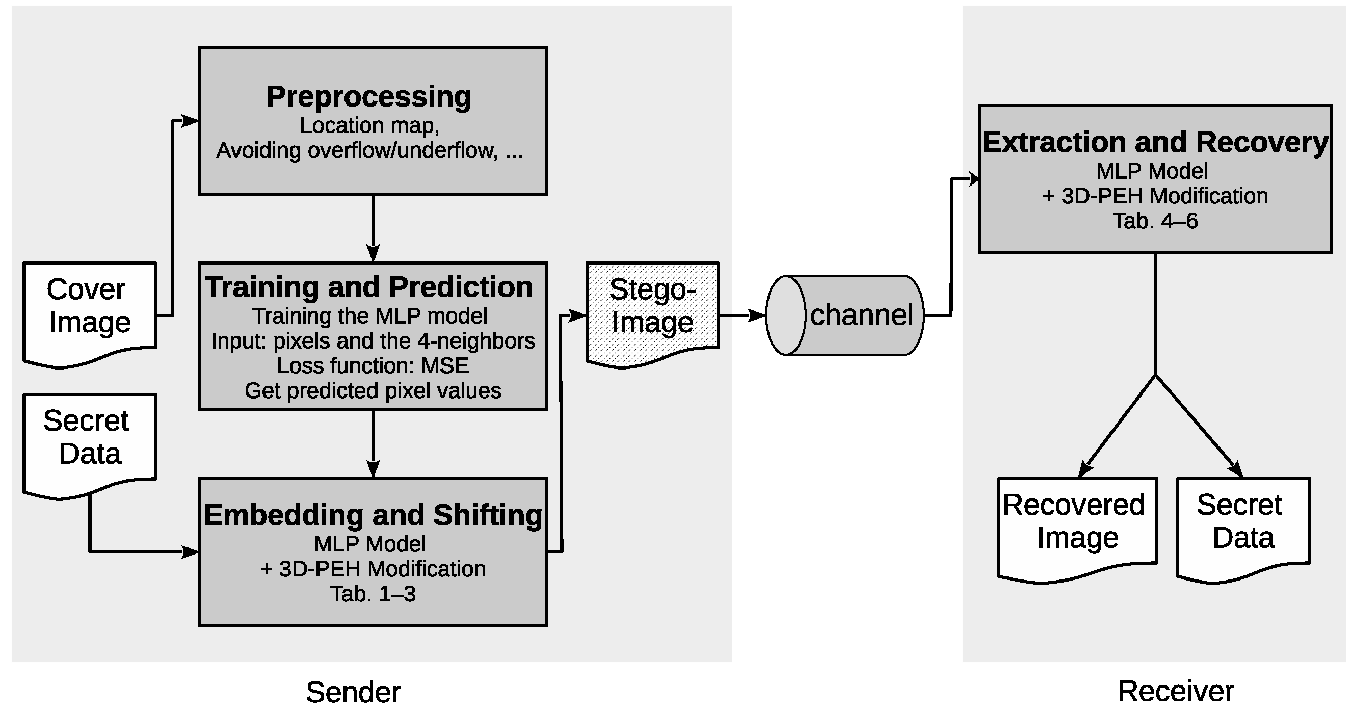
3. The Proposed Approach

In this section, we introduce our reversible data hiding scheme based on 3D-PEH modification and a MLP as the pixel value predictor. As the hypothesis in Section 1 states, we expect the performance of such a RDH scheme can be greatly enhanced by an accurate MLP predictor. The characteristics of the correlation between the image pixel value and the neighboring pixels is used, so that the accuracy of pixel prediction can be hopefully improved due to a better trained MLP model. This then leads to increased embedding capacity. Overall, our proposed method includes four parts: the pre-processing phase, the training and prediction phase, the embedding and shifting phase, and the extraction and recovery phase. The flowchart of the proposed method is shown in Figure 2. We specify the four phases in the following subsections.

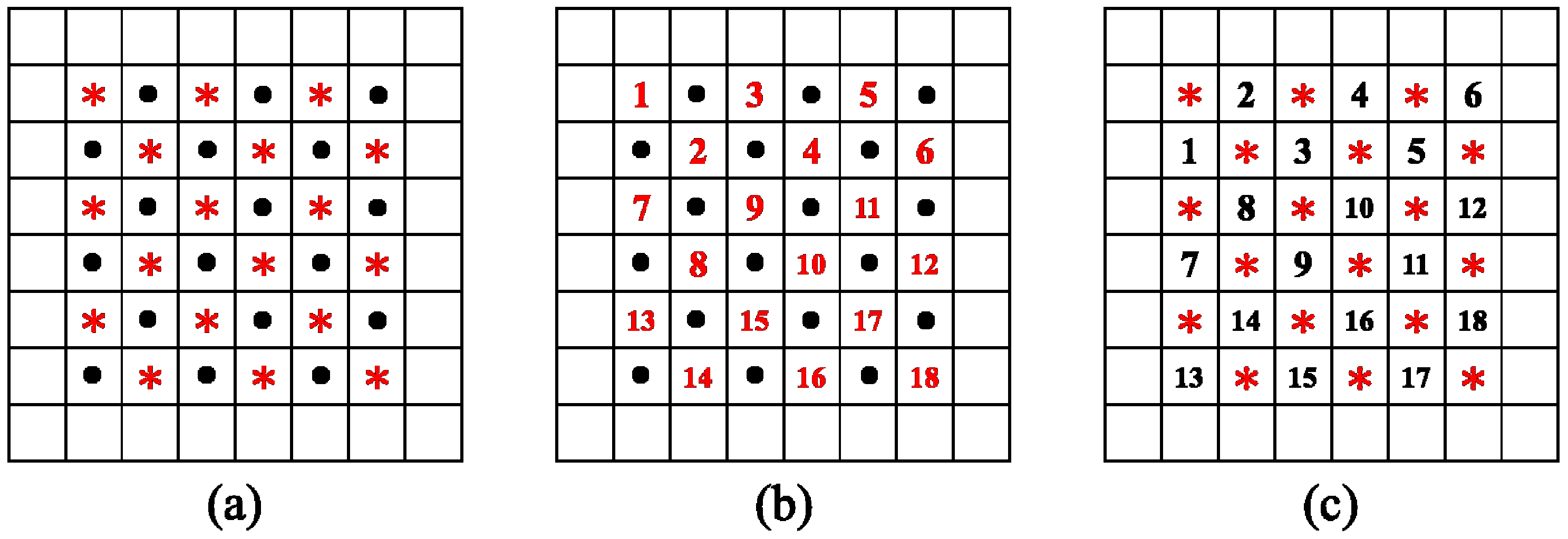
3.1. The Pre-Processing Phase

The pixel values of the cover image will be modified by $+1$ or $-1$ when the secret data embed based on 3D-PEH. Therefore, in order to avoid the overflow and underflow, the cover image will be pre-processed. Amend the pixel with value 0 to 1, and the pixel with value 255 to 254. Meanwhile, a location map is created to record these modified pixel positions. The location map is a binary sequence, which can be losslessly compressed to reduce its size. Then the secret data and the compressed location map are combined (hereinafter referred to as secret data); thereby, the pre-processing phase has been completed. After that, they will be embedded in the pre-processed cover image together.

3.2. The Training and Prediction Phase

The PEE method aims at the correlations between the pixels to derive accurate predictions where the prediction-errors are modified separately. However, the traditional PEE method uses the same algorithm to predict pixels for all images. This results in poor prediction accuracy and the prediction error increases as the image is relatively complex. Therefore, our proposed method, which leverages the power of trained MLP model, can predict the pixels of the cover image and significantly reduces the prediction-error so that the embedding capacity can be hopefully increased.

In the MLP training stage, except for pixels located in borders, the pixels are scanned from left to right and top to bottom to derive the cover sequence $(y_1,\dots ,y_n)$. Consider the four-neighbor tuple $(x_{\mathrm{top}},x_{\mathrm{bottom}},x_{\mathrm{left}},x_{\mathrm{right}}\}$ of a given pixel $y_i$, shown in the left part of the Figure 3. The four-neighbor tuple is used as input data of the neural network, and the desired output value is $y_i$.

The structure of an MLP neural network has one input layer, two hidden layers, and one output layer, as shown in Figure 3. The input of four-neighbor tuples $(x_{\mathrm{top}},x_{\mathrm{bottom}},x_{\mathrm{left}},x_{\mathrm{right}})$ from the cover image is fed into the input layer of the MLP. Between the input and output layers, there have 100 and 200 neurons in two hidden layers, respectively. After the information income is processed by the network, the output layer of the neural network provides one output ${\tilde{y}}_i$ as the predicted value by the MLP, and the corresponding $y_i$ in the cover image is used as reference data. We use the mean squared error (MSE) as the loss function which is calculated by taking the average squared difference between the predicted pixel value and the reference pixel value. The MSE function is defined as the Equation (1). Apparently, there is no prediction errors if and only if the MSE value is 0.

$$\mathrm{MSE}=\frac{1}{N}·\sum _{i=1}^N{({\tilde{y}}_i-y_i)}^2.$$

(1)

Here, N is the number of data points, ${\tilde{y}}_i$ is the value returned by the model, and $y_i$ is the actual value for data point. Based on those input and reference data, the MLP network is then trained with the loss function such that the edge weights of the MLP are optimized to best associate given neighborhoods with the reference pixel values.

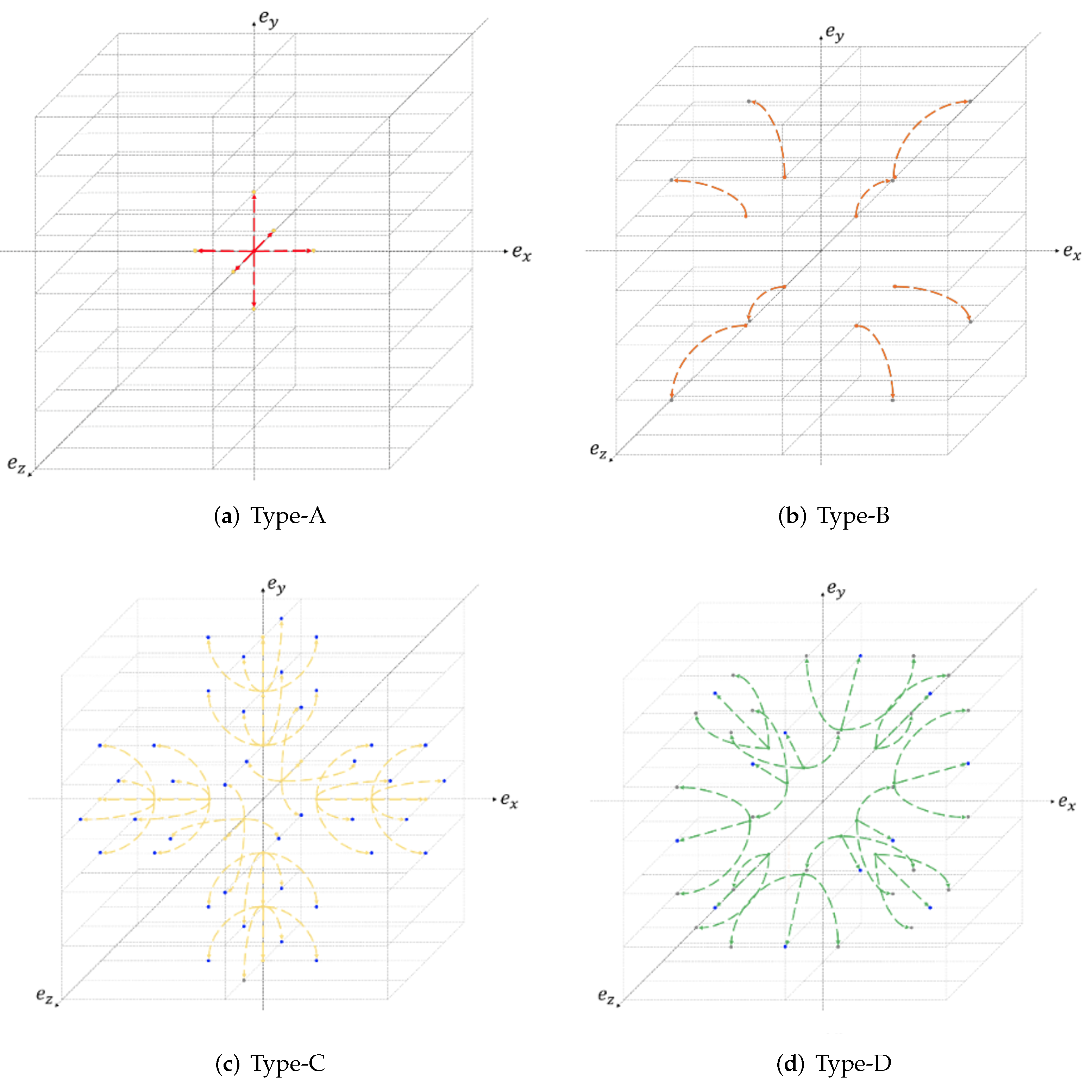
3.3. The Embedding and Shifting Phase

After the training and prediction phase is completed, the scheme enters the embedding and shifting phase. In order to embed the binary secret data in the cover image, the three-dimensional PEH (3D-PEH) modification is used for embedding and shifting. However, in the previous work on 3D-PEH modification, only the points located in the first octant of the three-dimensional coordinate system are modified. This way of hiding secrets did not make use of most of the space in the three-dimensional coordinate system for embedding; hence, the embeddable pixels are relatively less and a less embedding capacity of images is made. Instead, our proposed method embed secret data in eight octants of the three-dimensional space, so that we possibly exploit much more space than previous approaches.

We adopt rhombus prediction and double-layered embedding, the same as the way used in [5,24], for the implementation of the proposed method to generate non-overlapping prediction-error triple $(e_x,e_y,e_z)=(e_{3i-2},e_{3i-1},e_{3i})$ for feasible i (i.e., each pixel in the triple has four neighboring pixels). A 3D-PEH is generated by counting each non-overlapping prediction error triple, and the data embedding is realized by the obtained 3D-PEH modification using the designed reversible mapping. The data embedding procedure is briefly described as follows.

First, adopt double-layered embedding to divide the cover image into two sets denoted as “star”and “dot”(as shown in Figure 4a). The star and dot sets are embedded with half of the secret data, separately. Except for the pixels located in borders, the pixels of the star or dot set are scanned from left to right and top to bottom to derive the cover sequence $(p_1,\dots ,p_n)$. The scan orders for star and dot pixels are shown in Figure 4b,c.

Then, the 4-neighbor pixels of each $p_i$ are introduced to the trained MLP to obtain its predicted value ${\widehat{p}}_i$. The predicted value is used to determine the prediction-error sequence $(e_1,\dots ,e_n)$, and the sequence is divided into the prediction-error triples $e_x,e_y,e_z$. The prediction-error $e_i$ can be obtained as

$$e_i=p_i-{\widehat{p}}_i.$$

(2)

Lastly, modify each prediction-error triple $(e_x,e_y,e_z)$ to be $(e_x^{*},e_y^{*},e_z^{*})$ and get $({\tilde{p}}_x,{\tilde{p}}_y,{\tilde{p}}_z)=({\widehat{p}}_x+e_x^{*},{\widehat{p}}_y+e_y^{*},{\widehat{p}}_z+e_z^{*})$ to embed data based on the 3D-PEH in the method shown in

Table 3. Type A–C of the marked values of prediction-error triple $(e_x,e_y,e_z)$ and cover pixel triple $p_x,p_y,p_z$ in different types of the proposed method with embedding as the data embedding operations on $(e_x,e_y,e_z)$.

Type	$({\mathit{e}}_{\mathit{x}},{\mathit{e}}_{\mathit{y}},{\mathit{e}}_{\mathit{z}})$	Secret Bits	EC (bits)	$({\mathit{e}}_{\mathit{x}}^{*},{\mathit{e}}_{\mathit{y}}^{*},{\mathit{e}}_{\mathit{z}}^{*})$	$({\tilde{\mathit{p}}}_{\mathit{x}},{\tilde{\mathit{p}}}_{\mathit{y}},{\tilde{\mathit{p}}}_{\mathit{z}})$
A	$(e_x,e_y,e_z)=(0,0,0)$	$\left[0\right],\left[0\right],\left[0\right]$ $\left[0\right],\left[0\right],\left[1\right]$ $\left[0\right],\left[1\right],\left[0\right]$ $\left[0\right],\left[1\right],\left[1\right]$ $\left[1\right],\left[0\right],\left[0\right]$ $\left[1\right],\left[0\right],\left[1\right]$	3	$(0,0,0)$ $(0,0,1)$ $(0,1,0)$ $(0,-1,0)$ $(1,0,0)$ $(0,0,-1)$	$(p_x,p_y,p_z)$ $(p_x,p_y,p_z+1)$ $(p_x,p_y+1,p_z)$ $(p_x,p_y-1,p_z)$ $(p_x+1,p_y,p_z)$ $(p_x,p_y,p_z-1)$
A	$(e_x,e_y,e_z)=(0,0,0)$	$\left[1\right],\left[1\right]$	2	$(-1,0,0)$	$(p_x-1,p_y,p_z)$
B	$(e_x,e_y,e_z)=(\pm 1,\pm 1,\pm 1)$	$\left[0\right]$ $\left[1\right]$	1	$(\pm 1,\pm 1,\pm 1)$ $(\pm 2,\pm 2,\pm 2)$	$(p_x,p_y,p_z)$ $(p_x\pm 1,p_y\pm 1,p_z\pm 1)$
C	$e_x\ne 0$, $(e_y,e_z)=(0,0)$	$\left[1\right],\left[1\right],\left[1\right]$	3	$(e_x\pm 1,-1,0)$	$(p_x\pm 1,p_y-1,p_z)$
C	$e_x\ne 0$, $(e_y,e_z)=(0,0)$	$\left[0\right],\left[0\right]$ $\left[0\right],\left[1\right]$ $\left[1\right],\left[0\right]$ $\left[1\right],\left[1\right]$	2	$(e_x\pm 1,0,0)$ $(e_x\pm 1,0,1)$ $(e_x\pm 1,1,0)$ $(e_x\pm 1,0,-1)$	$(p_x\pm 1,p_y,p_z)$ $(p_x\pm 1,p_y,p_z+1)$ $(p_x\pm 1,p_y+1,p_z)$ $(p_x\pm 1,p_y,p_z-1)$
C	$e_y\ne 0$, $(e_x,e_z)=(0,0)$	$\left[1\right],\left[1\right],\left[1\right]$	3	$(-1,e_y\pm 1,0)$	$(p_x-1,p_y\pm 1,p_z)$
C	$e_y\ne 0$, $(e_x,e_z)=(0,0)$	$\left[0\right],\left[0\right]$ $\left[0\right],\left[1\right]$ $\left[1\right],\left[0\right]$ $\left[1\right],\left[1\right]$	2	$(0,e_y\pm 1,0)$ $(0,e_y\pm 1,1)$ $(1,e_y\pm 1,0)$ $(0,e_y\pm 1,-1)$	$(p_x,p_y\pm 1,p_z)$ $(p_x,p_y\pm 1,p_z+1)$ $(p_x\pm 1,p_y\pm 1,p_z)$ $(p_x,p_y\pm 1,p_z-1)$
C	$e_z\ne 0$, $(e_x,e_y)=(0,0)$	$\left[1\right],\left[1\right],\left[1\right]$	3	$(-1,0,e_z\pm 1)$	$(p_x-1,p_y,p_z\pm 1)$
C	$e_z\ne 0$, $(e_x,e_y)=(0,0)$	$\left[0\right],\left[0\right]$ $\left[0\right],\left[1\right]$ $\left[1\right],\left[0\right]$ $\left[1\right],\left[1\right]$	2	$(0,0,e_z\pm 1)$ $(0,1,e_z\pm 1)$ $(1,0,e_z\pm 1)$ $(0,-1,e_z\pm 1)$	$(p_x,p_y,p_z\pm 1)$ $(p_x,p_y+1,p_z\pm 1)$ $(p_x+1,p_y,p_z\pm 1)$ $(p_x,p_y-1,p_z\pm 1)$

,

Table 4. Type D–F of the marked values of prediction-error triple $(e_x,e_y,e_z)$ and cover pixel triple $p_x,p_y,p_z$ in different types of the proposed method with embedding as the data embedding operations on $(e_x,e_y,e_z)$.

Type	$({\mathit{e}}_{\mathit{x}},{\mathit{e}}_{\mathit{y}},{\mathit{e}}_{\mathit{z}})$	Secret Bits	EC (bits)	$({\mathit{e}}_{\mathit{x}}^{*},{\mathit{e}}_{\mathit{y}}^{*},{\mathit{e}}_{\mathit{z}}^{*})$	$({\tilde{\mathit{p}}}_{\mathit{x}},{\tilde{\mathit{p}}}_{\mathit{y}},{\tilde{\mathit{p}}}_{\mathit{z}})$
D	$(e_x,e_y,e_z)=(0,\pm 1,\pm 1)$	$\left[0\right],\left[0\right]$ $\left[0\right],\left[1\right]$ $\left[1\right],\left[0\right]$ $\left[1\right],\left[1\right]$	2	$(0,\pm 1,\pm 1)$ $(0,\pm 2,\pm 2)$ $(1,\pm 2,\pm 2)$ $(-1,\pm 2,\pm 2)$	$(p_x,p_y,p_z)$ $(p_x,p_y\pm 1,p_z\pm 1)$ $(p_x+1,p_y\pm 1,p_z\pm 1)$ $(p_x-1,p_y\pm 1,p_z\pm 1)$
D	$(e_x,e_y,e_z)=(\pm 1,0,\pm 1)$	$\left[0\right],\left[0\right]$ $\left[0\right],\left[1\right]$ $\left[1\right],\left[0\right]$ $\left[1\right],\left[1\right]$	2	$(\pm 1,0,\pm 1)$ $(\pm 2,0,\pm 2)$ $(\pm 2,1,\pm 2)$ $(\pm 2,-1,\pm 2)$	$(p_x,p_y,p_z)$ $(p_x\pm 1,p_y\pm 1,p_z)$ $(p_x\pm 1,p_y\pm 1,p_z+1)$ $(p_x\pm 1,p_y-1,p_z\pm 1)$
D	$(e_x,e_y,e_z)=(\pm 1,\pm 1,0)$	$\left[0\right],\left[0\right]$ $\left[0\right],\left[1\right]$ $\left[1\right],\left[0\right]$ $\left[1\right],\left[1\right]$	2	$(\pm 1,\pm 1,0)$ $(\pm 2,\pm 2,0)$ $(\pm 2,\pm 2,1)$ $(\pm 2,\pm 2,-1)$	$(p_x,p_y,p_z)$ $(p_x\pm 1,p_y\pm 1,p_z)$ $(p_x\pm 1,p_y\pm 1,p_z+1)$ $(p_x\pm 1,p_y\pm 1,p_z-1)$
E	$e_x=0$, $e_y,e_z\notin \{0,\pm 1\}$	$\left[0\right],\left[0\right]$ $\left[0\right],\left[1\right]$	2	$(0,e_y\pm 1,e_z\pm 1)$ $(1,e_y\pm 1,e_z\pm 1)$	$(p_x,p_y\pm 1,p_z\pm 1)$ $(p_x+1,p_y\pm 1,p_z\pm 1)$
E	$e_x=0$, $e_y,e_z\notin \{0,\pm 1\}$	$\left[1\right]$	1	$(-1,e_y\pm 1,e_z\pm 1)$	$(p_x-1,p_y\pm 1,p_z\pm 1)$
E	$e_y=0$, $e_x,e_z\notin \{0,\pm 1\}$	$\left[0\right],\left[0\right]$ $\left[0\right],\left[1\right]$	2	$(e_x\pm 1,0,e_z\pm 1)$ $(e_x\pm 1,1,e_z\pm 1)$	$(p_x\pm 1,p_y,p_z\pm 1)$ $(p_x\pm 1,p_y+1,p_z\pm 1)$
E	$e_y=0$, $e_x,e_z\notin \{0,\pm 1\}$	$\left[1\right]$	1	$(e_x\pm 1,-1,e_z\pm 1)$	$(p_x\pm 1,p_y-1,p_z\pm 1)$
E	$e_z=0$, $e_x,e_y\notin \{0,\pm 1\}$	$\left[0\right],\left[0\right]$ $\left[0\right],\left[1\right]$	2	$(e_x\pm 1,e_y\pm 1,0)$ $(e_x\pm 1,e_y\pm 1,1)$	$(p_x\pm 1,p_y\pm 1,p_z)$ $(p_x\pm 1,p_y\pm 1,p_z+1)$
E	$e_z=0$, $e_x,e_y\notin \{0,\pm 1\}$	$\left[1\right]$	1	$(e_x\pm 1,e_y\pm 1,-1)$	$(p_x\pm 1,p_y\pm 1,p_z-1)$
F	$|e_x|>1$, $(e_y,e_z)=(\pm 1,\pm 1)$	$\left[0\right]$ $\left[1\right]$	1	$(e_x\pm 1,\pm 1,\pm 1)$ $(e_x\pm 1,\pm 2,\pm 2)$	$(p_x\pm 1,p_y,p_z)$ $(p_x\pm 1,p_y\pm 1,p_z\pm 1)$
F	$|e_y|>1$, $(e_x,e_z)=(\pm 1,\pm 1)$	$\left[0\right]$ $\left[1\right]$	1	$(\pm 1,e_y\pm 1,\pm 1)$ $(\pm 2,e_y\pm 1,\pm 2)$	$(p_x,p_y\pm 1,p_z)$ $(p_x\pm 1,p_y\pm 1,p_z\pm 1)$
F	$|e_z|>1$, $(e_x,e_y)=(\pm 1,\pm 1)$	$\left[0\right]$ $\left[1\right]$	1	$(\pm 1,\pm 1,e_z\pm 1)$ $(\pm 2,\pm 2,e_z\pm 1)$	$(p_x,p_y,p_z\pm 1)$ $(p_x\pm 1,p_y\pm 1,p_z\pm 1)$

and

Table 5. Type G of the marked values of prediction-error triple $(e_x,e_y,e_z)$ and cover pixel triple $p_x,p_y,p_z$ in different types of the proposed method with shifting as the data embedding operations on $(e_x,e_y,e_z)$.

Type	$({\mathit{e}}_{\mathit{x}},{\mathit{e}}_{\mathit{y}},{\mathit{e}}_{\mathit{z}})$	Secret Bits	EC (bits)	$({\mathit{e}}_{\mathit{x}}^{*},{\mathit{e}}_{\mathit{y}}^{*},{\mathit{e}}_{\mathit{z}}^{*})$	$({\tilde{\mathit{p}}}_{\mathit{x}},{\tilde{\mathit{p}}}_{\mathit{y}},{\tilde{\mathit{p}}}_{\mathit{z}})$
G	$e_x,e_y,e_z\ne 0$, and $(e_x,e_y,e_z)\notin \mathrm{Type}B,F$	–	–	$(e_x\pm 1,e_y\pm 1,e_z\pm 1)$	$(p_x\pm 1,p_y\pm 1,p_z\pm 1)$

. The 3D-PEH mapping method is divided into seven types: Type A to Type G.

Figure 5 visualizes the mapping how the secret data are embedded. The goal of such visualization is to provide an intuitive way to verify the reversibility of the our proposed method. First of all, there are seven types of embedding in the proposed method, the mapping relationship of Type A, B, …, and G can be visualized as shown in Figure 5. An arrow with the starting point x to the end point y represents the data x transforms to the data y in this mapping. That is, the prediction-error groups $e_x,e_y,e_z$ and the cover pixel groups $p_x,p_y,p_z$ are modified by type A to type F according to the condition of the secret which will be embedded. For example, Type A could hide data by transforming $(0,0,0)$ into $(0,0,0)$, $(0,0,1)$, $(0,1,0)$, $(0,-1,0)$, $(1,0,0)$, $(0,0,-1)$, and $(-1,0,0)$. Therefore, Figure 5a shows the six arrows which starts from $(0,0,0)$ to the destinations $(0,0,0)$, $(0,0,1)$, $(0,1,0)$, $(0,-1,0)$, $(1,0,0)$, $(0,0,-1)$, and $(-1,0,0)$, respectively. Therefore, one can check if the mapping for data hiding is revertible by checking if one point in the mapping diagram can be reached by multiple points.

After the embedding and shifting phase, the stego-image embedded with secret data will be obtained. Then, the stego-image and the trained MLP model are sent to the receiver side through the communication channel.

Example 1.

Consider the cover image $P=${210, 99, 131, 65, 72, 162, 17, 19, 25, 161, 25, 71, 86, 95, 47}, the secret bits $S=\{0,0,0,1,1,0,1,1,1,1,0\}$, and the prediction error $E=\{0,0,0,0,0,0,1,1,-1,1,0,0,0,1,0\}$.

• Step 1:

  1. 

  Get the three bits from $E=\{\mathbf{0},\mathbf{0},\mathbf{0},0,0,0,1,1,-1,1,0,0,0,1,0\}$: $(e_x,e_y,e_z)=(0,0,0)$. This is a Type-A case.

  2. 

  Get three bits from $S=\{\mathbf{0},\mathbf{0},\mathbf{0},1,1,0,1,1,1,1,0\}$ if the first two bits are $\left[0\right],\left[0\right]$. Since the secret bits are $\left[0\right],\left[0\right],\left[0\right]$, we have $(e_x^{*},e_y^{*},e_z^{*})=(0,0,0)$.

  3. 

  Get three units from $P=\{\mathbf{210},\mathbf{99},\mathbf{131},65,72,162,17,19,25,161,25,71,86,95,47\}$ and derive $({\tilde{p}}_x,{\tilde{p}}_y,{\tilde{p}}_z)=(210,99,131)+(0,0,0)=(210,99,131)$.

  The results of this step are $E^{*}=\{0,0,0,\dots \}$ and ${\tilde{p}}_x=\{210,99,131,\dots \}$.
• Step 2:

  1. 

  Get three bits from $E=\{0,0,0,\mathbf{0},\mathbf{0},\mathbf{0},1,1,-1,1,0,0,0,1,0\}$: $(e_x,e_y,e_z)=(0,0,0)$. This is a Type-A case.

  2. 

  Get two bits from $S=\{0,0,0,\mathbf{1},\mathbf{1},0,1,1,1,1,0\}$. Since the secret bits are $\left[1\right],\left[1\right]$, we have $(e_x^{*},e_y^{*},e_z^{*})=(-1,0,0)$.

  3. 

  Get three units from $P=\{210,99,131,\mathbf{65},\mathbf{72},\mathbf{162},17,19,25,161,25,71,86,95,47\}$. and derive $({\tilde{p}}_x,{\tilde{p}}_y,{\tilde{p}}_z)=(65,72,162)+(-1,0,0)=(64,72,162)$.

  The results of this step are $E^{*}=\{0,0,0,-1,0,0,\dots \}$ and ${\tilde{p}}_x=\{210,99,131,64,72,162,\dots \}$.
• Step 3:

  1. 

  Get three bits from $E=\{0,0,0,0,0,0,\mathbf{1},\mathbf{1},-\mathbf{1},1,0,0,0,1,0\}$: $(e_x,e_y,e_z)=(1,1,-1)$. This is a Type-B case.

  2. 

  Get one bit from $S=\{0,0,0,1,1,\mathbf{0},1,1,1,1,0\}$. Since the secret bit is $\left[0\right]$, we have $(e_x^{*},e_y^{*},e_z^{*})=(1,1,-1)$.

  3. 

  Get three units from $P=\{210,99,131,65,72,162,\mathbf{17},\mathbf{19},\mathbf{25},161,25,71,86,95,47\}$ and derive $({\tilde{p}}_x,{\tilde{p}}_y,{\tilde{p}}_z)$= $(17,19,25)+(0,0,0)=(17,19,25)$.

  The results of this step are $E^{*}=\{0,0,0,-1,0,0,1,1,-1,\dots \}$ and ${\tilde{p}}_x=\{210,99,131,64,72,162,17,19,25,\dots \}$.
• Step 4:

  1. 

  Get three bits from $E=\{0,0,0,0,0,0,1,1,-1,\mathbf{1},\mathbf{0},\mathbf{0},0,1,0\}$: $(e_x,e_y,e_z)=(1,0,0)$. This is a Type-C case.

  2. 

  Get three bits from $S=\{0,0,0,1,1,0,\mathbf{1},\mathbf{1},\mathbf{1},1,0\}$ if the secret bits are $\left[1\right],\left[1\right],\left[1\right]$. Since the secret bit is $\left[1\right],\left[1\right],\left[1\right]$, we have $(e_x^{*},e_y^{*},e_z^{*})=(2,-1,0)$.

  3. 

  Get three units from $P=\{210,99,131,65,72,162,17,19,25,\mathbf{161},\mathbf{25},\mathbf{71},86,95,47\}$. and derive $({\tilde{p}}_x,{\tilde{p}}_y,{\tilde{p}}_z)=(161,25,71)+(1,-1,0)=(162,24,71)$

  The results of this step are $E^{*}=\{0,0,0,-1,0,0,1,1,-1,2,-1,0,\dots \}$ and ${\tilde{p}}_x=\{210,99,131,$$64,72,162,17,19,25,162,24,71,\dots \}$.
• Step 5:

  1. 

  Get three bits from $E=\{0,0,0,0,0,0,1,1,-1,1,0,0,\mathbf{0},\mathbf{1},\mathbf{0}\}$: $(e_x,e_y,e_z)=(0,1,0)$. This is a Type-C case.

  2. 

  Get two bits from $S=\{0,0,0,1,1,0,1,1,1,\mathbf{1},\mathbf{0}\}$ if the secret bits are not $\left[1\right],\left[1\right],\left[1\right]$. Since the secret bit is $\left[1\right],\left[0\right]$, we have $(e_x^{*},e_y^{*},e_z^{*})=(1,2,0)$.

  3. 

  Get three units from $P=\{210,99,131,65,72,162,17,19,25,161,25,71,\mathbf{86},\mathbf{95},\mathbf{47}\}$. and derive $({\tilde{p}}_x,{\tilde{p}}_y,{\tilde{p}}_z)=(86,95,47)+(1,1,0)=(87,96,47)$.

  The results of this step are $E^{*}=\{0,0,0,-1,0,0,1,1,-1,2,-1,0,1,2,0\}$ and ${\tilde{p}}_x=\{210,99,131,64,72,162,17,19,25,87,96,47\}$.

3.4. The Extraction and Recovery Phase

Through the communication channel, the stego-image and the trained MLP model are received. Next, we consider the secret data extraction from the stego-image and the stego-image recovery. The scheme then enters the extraction and recovery phase.

In the extraction and recovery stage, the procedure of the secret data extraction and the stego-image recovery is similar to the procedure of embedding and shifting. The secret data extraction process is briefly described as follows.

First, rhombus prediction and double-layered embedding is adopted to divide the stego-image into two sets denoted as “star”and “dot” (as shown in Figure 4a), and half of the secret data will be extracted from the star and dot sets, respectively. Except for the pixels located in borders, the pixels of the star or dot set are scanned from top-left to bottom-right to derive the stego sequence $(p_1^{\prime },\dots ,p_n^{\prime })$.

Then, the 4-neighbor dots of each $p_i^{\prime }$ are introduced to the trained MLP to obtain its predicted value $\widehat{p_i^{\prime }}$. The predicted value is used to determine the prediction-error sequence $(e_1^{\prime },\dots ,e_n^{\prime })$, and the sequence is divided into the prediction-error triples $(e_x^{\prime },e_y^{\prime },e_z^{\prime })$. The prediction-error $e_i^{\prime }$ can be obtained as

$$e_i^{\prime }=p_i^{\prime }-{\widehat{p^{\prime }}}_i.$$

Finally, each recovered triple $(p_x^{\prime },p_y^{\prime },p_z^{\prime })$ is extracted based on the 3D-PEH as the method shown in

Table 6. Type $A^{\prime }$–$C^{\prime }$ of the The extracted secret bits and the recovered values of prediction-error triple $(e_x^{\prime },e_y^{\prime },e_z^{\prime })$ and stego pixel triple $(p_x^{\prime },p_y^{\prime },p_z^{\prime })$ in different types of the proposed method with embedding as the data embedding operations on $(e_x^{\prime },e_y^{\prime },e_z^{\prime })$.

Type	$({\mathit{e}}_{\mathit{x}}^{\prime },{\mathit{e}}_{\mathit{y}}^{\prime },{\mathit{e}}_{\mathit{z}}^{\prime })$	Extracted Secret Bits	$({\mathit{e}}_{\mathit{x}},{\mathit{e}}_{\mathit{y}},{\mathit{e}}_{\mathit{z}})$	$({\mathit{p}}_{\mathit{x}},{\mathit{p}}_{\mathit{y}},{\mathit{p}}_{\mathit{z}})$
$A^{\prime }$	$(e_x^{\prime },e_y^{\prime },e_z^{\prime })=(0,0,0)$ $(e_x^{\prime },e_y^{\prime },e_z^{\prime })=(0,0,1)$ $(e_x^{\prime },e_y^{\prime },e_z^{\prime })=(0,1,0)$ $(e_x^{\prime },e_y^{\prime },e_z^{\prime })=(0,-1,0)$ $(e_x^{\prime },e_y^{\prime },e_z^{\prime })=(1,0,0)$ $(e_x^{\prime },e_y^{\prime },e_z^{\prime })=(0,0,-1)$ $(e_x^{\prime },e_y^{\prime },e_z^{\prime })=(0,-1,0)$	$\left[0\right],\left[0\right],\left[0\right]$ $\left[0\right],\left[0\right],\left[1\right]$ $\left[0\right],\left[1\right],\left[0\right]$ $\left[0\right],\left[1\right],\left[1\right]$ $\left[1\right],\left[0\right],\left[0\right]$ $\left[1\right],\left[0\right],\left[1\right]$ $\left[1\right],\left[1\right]$	$(0,0,0)$	$(p_x^{\prime },p_y^{\prime },p_z^{\prime })$ $(p_x^{\prime },p_y^{\prime },p_z^{\prime }-1)$ $(p_x^{\prime },p_y^{\prime }-1,p_z^{\prime })$ $(p_x^{\prime },p_y^{\prime }+1,p_z^{\prime })$ $(p_x^{\prime }-1,p_y^{\prime },p_z^{\prime })$ $(p_x^{\prime },p_y^{\prime },p_z^{\prime }+1)$ $(p_x^{\prime },p_y^{\prime }+1,p_z^{\prime }+1)$
$B^{\prime }$	$(e_x^{\prime },e_y^{\prime },e_z^{\prime })=(\pm 1,\pm 1,\pm 1)$ $(e_x^{\prime },e_y^{\prime },e_z^{\prime })=(\pm 2,\pm 2,\pm 2)$	$\left[0\right]$ $\left[1\right]$	$(\pm 1,\pm 1,\pm 1)$	$(p_x^{\prime },p_y^{\prime },p_z^{\prime })$ $(p_x^{\prime }\pm 1,p_y^{\prime }\pm 1,p_z^{\prime }\pm 1)$
$C^{\prime }$	$|e_x^{\prime }|>1$, $(e_y^{\prime },e_z^{\prime })=(-1,0)$ $|e_x^{\prime }|>1$, $(e_y^{\prime },e_z^{\prime })=(0,0)$ $|e_x^{\prime }|>1$, $(e_y^{\prime },e_z^{\prime })=(0,1)$ $|e_x^{\prime }|>1$, $(e_y^{\prime },e_z^{\prime })=(1,0)$ $|e_x^{\prime }|>1$, $(e_y^{\prime },e_z^{\prime })=(0,-1)$	$\left[1\right]$, $\left[1\right]$, $\left[1\right]$ $\left[0\right],\left[0\right]$ $\left[0\right],\left[1\right]$ $\left[1\right],\left[0\right]$ $\left[1\right],\left[1\right]$	$(e_x^{\prime }\pm 1,0,0)$	$(p_x^{\prime }\pm 1,p_y^{\prime }+1,p_z^{\prime })$ $(p_x^{\prime }\pm 1,p_y^{\prime },p_z^{\prime })$ $(p_x^{\prime }\pm 1,p_y^{\prime },p_z^{\prime }-1)$ $(p_x^{\prime }\pm 1,p_y^{\prime }-1,p_z^{\prime })$ $(p_x^{\prime }\pm 1,p_y^{\prime },p_z^{\prime }+1)$
$C^{\prime }$	$|e_y^{\prime }|>1$, $(e_x^{\prime },e_z^{\prime })=(-1,0)$ $|e_y^{\prime }|>1$, $(e_x^{\prime },e_z^{\prime })=(0,0)$ $|e_y^{\prime }|>1$, $(e_x^{\prime },e_z^{\prime })=(0,1)$ $|e_y^{\prime }|>1$, $(e_x^{\prime },e_z^{\prime })=(1,0)$ $|e_y^{\prime }|>1$, $(e_x^{\prime },e_z^{\prime })=(0,-1)$	$\left[1\right]$, $\left[1\right]$, $\left[1\right]$ $\left[0\right],\left[0\right]$ $\left[0\right],\left[1\right]$ $\left[1\right],\left[0\right]$ $\left[1\right],\left[1\right]$	$(0,e_y^{\prime }\pm 1,0)$	$(p_x^{\prime }+1,p_y^{\prime }\pm 1,p_z^{\prime })$ $(p_x^{\prime },p_y^{\prime }\pm 1,p_z^{\prime })$ $(p_x^{\prime },p_y^{\prime }\pm 1,p_z^{\prime }-1)$ $(p_x^{\prime }-1,p_y^{\prime }\pm 1,p_z^{\prime })$ $(p_x^{\prime },p_y^{\prime }\pm 1,p_z^{\prime }+1)$
$C^{\prime }$	$|e_z^{\prime }|>1$, $(e_x^{\prime },e_y^{\prime })=(-1,0)$ $|e_z^{\prime }|>1$, $(e_x^{\prime },e_y^{\prime })=(0,0)$ $|e_z^{\prime }|>1$, $(e_x^{\prime },e_y^{\prime })=(0,1)$ $|e_z^{\prime }|>1$, $(e_x^{\prime },e_y^{\prime })=(1,0)$ $|e_z^{\prime }|>1$, $(e_x^{\prime },e_y^{\prime })=(0,-1)$	$\left[1\right]$, $\left[1\right]$, $\left[1\right]$ $\left[0\right],\left[0\right]$ $\left[0\right],\left[1\right]$ $\left[1\right],\left[0\right]$ $\left[1\right],\left[1\right]$	$(0,0,e_z^{\prime }\pm 1)$	$(p_x^{\prime }+1,p_y^{\prime },p_z^{\prime }\pm 1)$ $(p_x^{\prime },p_y^{\prime },p_z^{\prime }\pm 1)$ $(p_x^{\prime },p_y^{\prime }-1,p_z^{\prime }\pm 1)$ $(p_x^{\prime }-1,p_y^{\prime },p_z^{\prime }\pm 1)$ $(p_x^{\prime },p_y^{\prime }+1,p_z^{\prime }\pm 1)$

,

Table 7. Type $D^{\prime }$–$F^{\prime }$ of the the extracted secret bits and the recovered values of prediction-error triple $(e_x^{\prime },e_y^{\prime },e_z^{\prime })$ and stego pixel triple $(p_x^{\prime },p_y^{\prime },p_z^{\prime })$ in different types of the proposed method with embedding as the data embedding operations on $(e_x^{\prime },e_y^{\prime },e_z^{\prime })$.

Type	$({\mathit{e}}_{\mathit{x}}^{\prime },{\mathit{e}}_{\mathit{y}}^{\prime },{\mathit{e}}_{\mathit{z}}^{\prime })$	Extracted Secret Bits	$({\mathit{e}}_{\mathit{x}},{\mathit{e}}_{\mathit{y}},{\mathit{e}}_{\mathit{z}})$	$({\mathit{p}}_{\mathit{x}},{\mathit{p}}_{\mathit{y}},{\mathit{p}}_{\mathit{z}})$
$D^{\prime }$	$(e_x^{\prime },e_y^{\prime },e_z^{\prime })=(0,\pm 1,\pm 1)$ $(e_x^{\prime },e_y^{\prime },e_z^{\prime })=(0,\pm 2,\pm 2)$ $(e_x^{\prime },e_y^{\prime },e_z^{\prime })=(1,\pm 2,\pm 2)$ $(e_x^{\prime },e_y^{\prime },e_z^{\prime })=(-1,\pm 2,\pm 2)$	$\left[0\right],\left[0\right]$ $\left[0\right],\left[1\right]$ $\left[1\right],\left[0\right]$ $\left[1\right],\left[1\right]$	$(0,\pm 1,\pm 1)$	$(p_x^{\prime },p_y^{\prime },p_z^{\prime })$ $(p_x^{\prime },p_y^{\prime }\pm 1,p_z^{\prime }\pm 1)$ $(p_x^{\prime }-1,p_y^{\prime }\pm 1,p_z^{\prime }\pm 1)$ $(p_x^{\prime }+1,p_y^{\prime }\pm 1,p_z^{\prime }\pm 1)$
$D^{\prime }$	$(e_x^{\prime },e_y^{\prime },e_z^{\prime })=(\pm 1,0,\pm 1)$ $(e_x^{\prime },e_y^{\prime },e_z^{\prime })=(\pm 2,0,\pm 2)$ $(e_x^{\prime },e_y^{\prime },e_z^{\prime })=(\pm 2,1,\pm 2)$ $(e_x^{\prime },e_y^{\prime },e_z^{\prime })=(\pm 2,-1,\pm 2)$	$\left[0\right],\left[0\right]$ $\left[0\right],\left[1\right]$ $\left[1\right],\left[0\right]$ $\left[1\right],\left[1\right]$	$(\pm 1,0,\pm 1)$	$(p_x^{\prime },p_y^{\prime },p_z^{\prime })$ $(p_x^{\prime }\pm 1,p_y^{\prime },p_z^{\prime }\pm 1)$ $(p_x^{\prime }\pm 1,p_y^{\prime }-1,p_z^{\prime }\pm 1)$ $(p_x^{\prime }\pm 1,p_y^{\prime }+1,p_z^{\prime }\pm 1)$
$D^{\prime }$	$(e_x^{\prime },e_y^{\prime },e_z^{\prime })=(\pm 1,\pm 1,0)$ $(e_x^{\prime },e_y^{\prime },e_z^{\prime })=(\pm 2,\pm 2,0)$ $(e_x^{\prime },e_y^{\prime },e_z^{\prime })=(\pm 2,\pm 2,1)$ $(e_x^{\prime },e_y^{\prime },e_z^{\prime })=(\pm 2,\pm 2,-1)$	$\left[0\right],\left[0\right]$ $\left[0\right],\left[1\right]$ $\left[1\right],\left[0\right]$ $\left[1\right],\left[1\right]$	$(\pm 1,\pm 1,0)$	$(p_x^{\prime },p_y^{\prime },p_z^{\prime })$ $(p_x^{\prime }\pm 1,p_y^{\prime }\pm 1,p_z^{\prime })$ $(p_x^{\prime }\pm 1,p_y^{\prime }\pm 1,p_z^{\prime }-1)$ $(p_x^{\prime }\pm 1,p_y^{\prime }\pm 1,p_z^{\prime }+1)$
$E^{\prime }$	$e_x^{\prime }=0$, $|e_y^{\prime }|>1$ $e_x^{\prime }=1$, $|e_z^{\prime }|>1$ $e_x^{\prime }=-1$, $(e_y^{\prime },e_z^{\prime })\ne (\pm 2,\pm 2)$	$\left[0\right],\left[0\right]$ $\left[0\right],\left[1\right]$ $\left[1\right]$	$(0,e_y^{\prime }\pm 1,e_z^{\prime }\pm 1)$	$(p_x^{\prime },p_y^{\prime }\pm 1,p_z^{\prime }\pm 1)$ $(p_x^{\prime }-1,p_y^{\prime }\pm 1,p_z^{\prime }\pm 1)$ $(p_x^{\prime },p_y^{\prime }\pm 1,p_z^{\prime }\pm 1)$
$E^{\prime }$	$e_y^{\prime }=0$, $|e_x^{\prime }|>1$ $e_y^{\prime }=1$, $|e_y^{\prime }|>1$ $e_y^{\prime }=-1$, $(e_x^{\prime },e_z^{\prime })\ne (\pm 2,\pm 2)$	$\left[0\right],\left[0\right]$ $\left[0\right],\left[1\right]$ $\left[1\right]$	$(e_x^{\prime }\pm 1,0,e_z^{\prime }\pm 1)$	$(p_x^{\prime }\pm 1,p_y^{\prime },p_z^{\prime }\pm 1)$ $(p_x^{\prime }\pm 1,p_y^{\prime }-1,p_z^{\prime }\pm 1)$ $(p_x^{\prime }\pm 1,p_y^{\prime }+1,p_z^{\prime }\pm 1)$
$E^{\prime }$	$e_z^{\prime }=0$, $|e_x^{\prime }|>1$ $e_z^{\prime }=1$, $|e_y^{\prime }|>1$ $e_z^{\prime }=-1$, $(e_x^{\prime },e_y^{\prime })\ne (\pm 2,\pm 2)$	$\left[0\right],\left[0\right]$ $\left[0\right],\left[1\right]$ $\left[1\right]$	$(e_x^{\prime }\pm 1,e_y^{\prime }\pm 1,0)$	$(p_x^{\prime }\pm 1,p_y^{\prime }\pm 1,p_z^{\prime })$ $(p_x^{\prime }\pm 1,p_y^{\prime }\pm 1,p_z^{\prime }-1)$ $(p_x^{\prime }\pm 1,p_y^{\prime }\pm 1,p_z^{\prime }+1)$
$F^{\prime }$	$|e_x^{\prime }|>2$, $(e_y^{\prime },e_z^{\prime })=(\pm 1,\pm 1)$ $|e_x^{\prime }|>2$, $(e_y^{\prime },e_z^{\prime })=(\pm 2,\pm 2)$	$\left[0\right]$ $\left[1\right]$	$(e_x^{\prime }\pm 1,\pm 1,\pm 1)$	$(p_x^{\prime }\pm 1,p_y^{\prime },p_z^{\prime })$ $(p_x^{\prime }\pm 1,p_y^{\prime }\pm 1,p_z^{\prime }\pm 1)$
$F^{\prime }$	$|e_y^{\prime }|>2$, $(e_x^{\prime },e_z^{\prime })=(\pm 1,\pm 1)$ $|e_y^{\prime }|>2$, $(e_x^{\prime },e_z^{\prime })=(\pm 2,\pm 2)$	$\left[0\right]$ $\left[1\right]$	$(\pm 1,e_y^{\prime }\pm 1,\pm 1)$	$(p_x^{\prime },p_y^{\prime }\pm 1,p_z^{\prime })$ $(p_x^{\prime }\pm 1,p_y^{\prime }\pm 1,p_z^{\prime }\pm 1)$
$F^{\prime }$	$|e_z^{\prime }|>2$, $(e_x^{\prime },e_y^{\prime })=(\pm 1,\pm 1)$ $|e_z^{\prime }|>2$, $(e_x^{\prime },e_y^{\prime })=(\pm 2,\pm 2)$	$\left[0\right]$ $\left[1\right]$	$(\pm 1,\pm 1,e_z^{\prime }\pm 1)$	$(p_x^{\prime },p_y^{\prime },p_z^{\prime }\pm 1)$ $(p_x^{\prime }\pm 1,p_y^{\prime }\pm 1,p_z^{\prime }\pm 1)$

and

Table 8. Type $G^{\prime }$ of the The extracted secret bits and the recovered values of prediction-error triple $(e_x^{\prime },e_y^{\prime },e_z^{\prime })$ and stego pixel triple $p_x^{\prime },p_y^{\prime },p_z^{\prime }$ in different types of the proposed method with no embedded data bit on $(e_x^{\prime },e_y^{\prime },e_z^{\prime })$.

Type	$({\mathit{e}}_{\mathit{x}}^{\prime },{\mathit{e}}_{\mathit{y}}^{\prime },{\mathit{e}}_{\mathit{z}}^{\prime })$	Extracted Secret Bits	$({\mathit{e}}_{\mathit{x}},{\mathit{e}}_{\mathit{y}},{\mathit{e}}_{\mathit{z}})$	$({\mathit{p}}_{\mathit{x}},{\mathit{p}}_{\mathit{y}},{\mathit{p}}_{\mathit{z}})$
$G^{\prime }$	$|e_x^{\prime }|>1$, $|e_y^{\prime }|>1$, $|e_z^{\prime }|>1$, $(e_x^{\prime },e_y^{\prime },e_z^{\prime })\notin TypeB,F$	no embedded data bit	$(e_x^{\prime }\pm 1,e_y^{\prime }\pm 1,e_z^{\prime }\pm 1)$	$(p_x^{\prime }\pm 1,p_y^{\prime }\pm 1,p_z^{\prime }\pm 1)$

. The 3D-PEH recovery method is divided into seven types: Type $A^{\prime }$ to Type $G^{\prime }$. Besides, $(e_x^{\prime },e_y^{\prime },e_z^{\prime })$ should be the prediction-errors between the “marked pixels” (in the stego-image) and the prediction of the “marked pixels”. When the prediction-error $e_i^{\prime }$ is 1, the recovered value is $p_i=p_i^{\prime }-1$, and when the prediction-error $e_i^{\prime }$ is $-1$, the recovered value is $p_i=p_i^{\prime }+1$.

The secret data bits are extracted by type $A^{\prime }$ to type $G^{\prime }$ according to the condition of the prediction-error group and the stego pixel group $(p_x^{\prime },p_y^{\prime },p_z^{\prime })$ is recovered to the recover pixel groups that have the same pixel values as the cover pixel groups $(p_x,p_y,p_z)$. In addition, the type $G^{\prime }$ has no embedded data bits, so only recover the stego pixel groups to the recover pixel groups without secret data extraction.

Through the extraction and recovery phase, the secret data and the recovered image are obtained.

Example 2.

Let $P^{{}^{\prime }}=\{210,99,131,64,72,162,17,19,25,162,24,71,87,96,47\}$, and $E^{{}^{\prime }}=\{0,0,0,-1,0,0,1,1,-1,2,-1,0,1,2,0\}$.

• Step 1:

  1. 

  Get the three bits from $E^{{}^{\prime }}=\{\mathbf{0},\mathbf{0},\mathbf{0},-1,0,0,1,1,-1,2,-1,0,1,2,0\}$: $(e_x^{{}^{\prime }},e_y^{{}^{\prime }},e_z^{{}^{\prime }})=(0,0,0)$. This is a Type-$A^{{}^{\prime }}$ case. The extracted secret bits are $(0,0,0)$.

  2. 

  Get three bits from $P^{{}^{\prime }}=\{\mathbf{210},\mathbf{99},\mathbf{131},64,72,162,17,19,25,162,24,71,87,96,47\}$. Then, we can derive $(p_x,p_y,p_z)=(210,99,131)$.

  The results of this step are $S=\{0,0,0,\dots \}$ and $P=\{210,99,131,\dots \}$.
• Step 2:

  1. 

  Get the three bits from $E^{{}^{\prime }}=\{0,0,0,-\mathbf{1},\mathbf{0},\mathbf{0},1,1,-1,2,-1,0,1,2,0\}$: $(e_x^{{}^{\prime }},e_y^{{}^{\prime }},e_z^{{}^{\prime }})=(-1,0,0)$. This is a Type-$A^{{}^{\prime }}$ case. The extracted secret bits are $\left[1\right],\left[1\right]$.

  2. 

  Get three bits from $P^{{}^{\prime }}=\{210,99,131,\mathbf{64},\mathbf{72},\mathbf{162},17,19,25,162,24,71,87,96,47\}$. Then, we can derive $(p_x,p_y,p_z)=(64+1,72,162)=(65,72,162)$.

  The results of this step are $S=\{0,0,0,1,1,\dots \}$ and $P=\{210,99,131,65,72,162\dots \}$.
• Step 3:

  1. 

  Get the three bits from $E^{{}^{\prime }}=\{0,0,0,-1,0,0,\mathbf{1},\mathbf{1},-\mathbf{1},2,-1,0,1,2,0\}$: $(e_x^{{}^{\prime }},e_y^{{}^{\prime }},e_z^{{}^{\prime }})=(1,1,-1)$. This is a Type-$B^{{}^{\prime }}$ case. The extracted secret bits are $\left[0\right]$.

  2. 

  Get three bits from $P^{{}^{\prime }}=\{210,99,131,64,72,162,\mathbf{17},\mathbf{19},\mathbf{25},162,24,71,87,96,47\}$. Then, we can derive $(p_x,p_y,p_z)=(17,19,25)$.

  The results of this step are $S=\{0,0,0,1,1,0,\dots \}$ and $P=\{210,99,131,65,72,162,17,19,25\dots \}$.
• Step 4:

  1. 

  Get the three bits from $E^{{}^{\prime }}=\{0,0,0,-1,0,0,1,1,-1,\mathbf{2},-\mathbf{1},\mathbf{0},1,2,0\}$: $(e_x^{{}^{\prime }},e_y^{{}^{\prime }},e_z^{{}^{\prime }})=(2,-1,0)$. This is a Type-$C^{{}^{\prime }}$ case. The extracted secret bits are $\left[1\right],\left[1\right],\left[1\right]$.

  2. 

  Get three bits from $P^{{}^{\prime }}=\{210,99,131,64,72,162,17,19,25,\mathbf{162},\mathbf{24},\mathbf{71},87,96,47\}$. Then, we can derive $(p_x,p_y,p_z)=(162-1,24+1,71)=(161,25,71)$.

  The results of this step are $S=\{0,0,0,1,1,0,1,1,1,\dots \}$ and $P=\{210,99,131,65,72,162,17,19,25,161,25,71\dots \}$.
• Step 5:

  1. 

  Get the three bits from $E^{{}^{\prime }}=\{0,0,0,-1,0,0,1,1,-1,2,-1,0,\mathbf{1},\mathbf{2},\mathbf{0}\}$: $(e_x^{{}^{\prime }},e_y^{{}^{\prime }},e_z^{{}^{\prime }})=(1,2,0)$. This is a Type-$C^{{}^{\prime }}$ case. The extracted secret bits are $\left[1\right],\left[0\right]$.

  2. 

  Get three bits from $P^{{}^{\prime }}=\{210,99,131,64,72,162,17,19,25,162,24,71,\mathbf{87},\mathbf{96},\mathbf{47}\}$. Then, we can derive $(p_x,p_y,p_z)=(87-1,96-1,47)=(86,95,47)$.

  The results of this step are $S=\{0,0,0,1,1,0,1,1,1,1,0\}$ and $P=\{210,99,131,65,72,162,17,19,25,161,25,71,86,95,47\}$.

4. Computational Complexity

Assume that the image has height M and width N respectively. In the pre-processing phase (where a lossless compression is used for the location map; however, we can assume that it can be done in time linearly in the number of pixels if we do not require the space usage as small as possible), training-and-prediction phase, embedding-and-shifting phase and extraction and recovery phase, the computational complexity is basically $O\left(MN\right)$ because there are $O\left(MN\right)$ pixels to be scanned for a constant number of times. We remark here that though the structure of the MLP neural network is fixed so that this part contributes a constant factor in the complexity, such a constant factor hidden in the asymptotic notation can actually be huge. More specifically, for each input data point (i.e., a set of four pixels) fed to the input layer of the MLP neural network in one iteration, there are $100\times 200$ multiplications required to compute the activation of all the neurons.

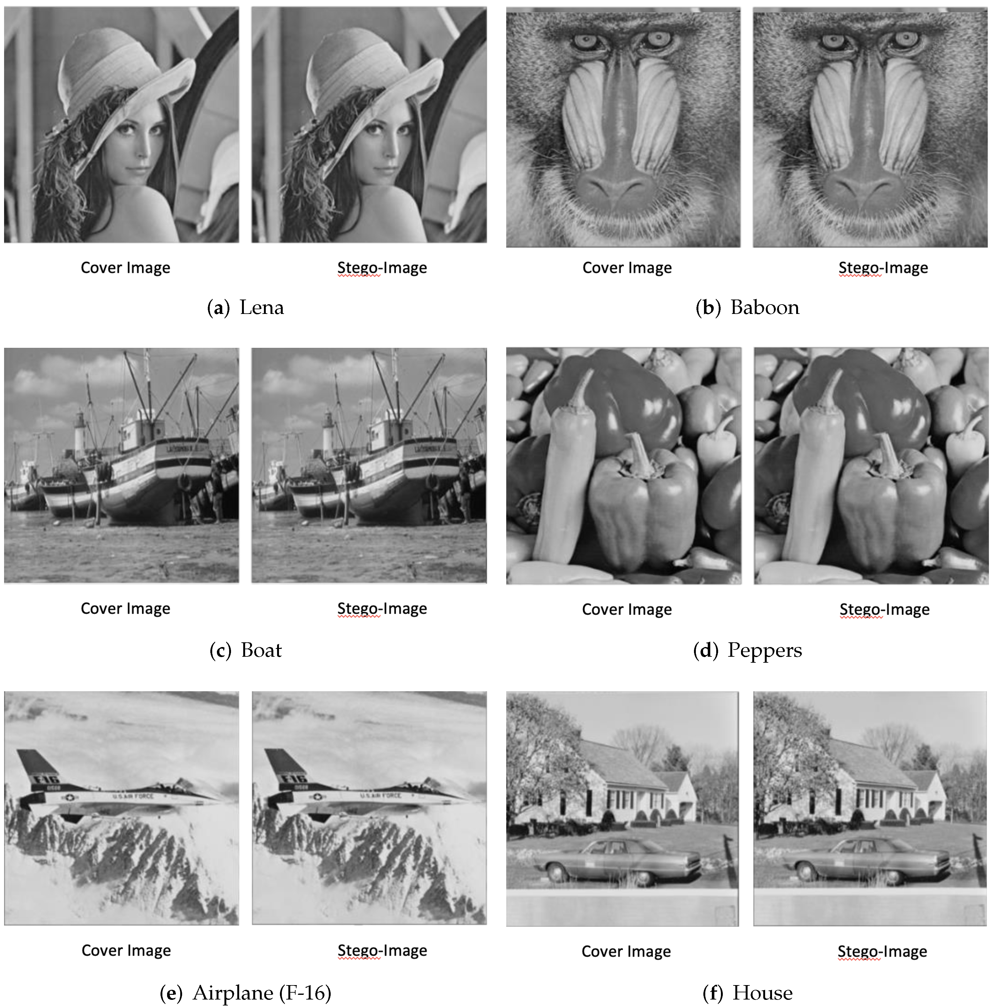
5. Experimental Results

The experimental results are shown in this section. Six grayscale images of size 512-by-512, including Lena, Baboon, Boat, Peppers, Airplane (F-16), and House, are used in our experiments. The cover images and the stego-images which are embedded 10,000 bits of secret data are shown in Figure 6. In addition, the variations in image quality under different embedding capacities are compared (as shown in Figure 7). The most common strategy to measure the image quality is the calculation of Peak Signal to Noise Ratio (PSNR) function which is defined as

$$\begin{array}{ccc}\hfill \mathrm{PSNR}& =& 10·{log}_{10}\left(\frac{255·255}{MSE}\right),\hfill \\ \hfill \mathrm{MSE}& =& \frac{1}{MN}·\sum _{i=1}^M\sum _{j=1}^N{(x_{i,j}-x_{i,j}^{\prime })}^2.\hfill \end{array}$$

The results of the testing image (Lena) is presented in Figure 7. In addition, from the line chart can be observed that when the embedding capacity is less than 60,000 bits, the PSNR will decrease steadily. However, when the embedding capacity is more than 60,000 bits, PSNR will begin to decline relatively quickly.

5.1. Performance Comparison between the Proposed Method and Baseline Approaches

In this subsection, the proposed method is compared with the previously mentioned schemes. The compared results divide into two parts: maximum embedding capacity and embedding capability in different embedding capacities. The comparison results show that the proposed method has better embedding capacity, and the image qualities are still maintained well.

5.1.1. Maximum Embedding Capacity

We compared the embedding capacity and the image quality when the cover image was embedded once from beginning to end. The comparison is between the proposed method and the methods of Ni et al. [46], Lee et al. [47], Li et al. [21], and Cai et al. [5]. Shown in

Table 9. Comparison of maximum embedding capacity (bits) for six test images between the proposed method and the methods of Ni et al. [46], Lee et al. [47], Li et al. [21], and Cai et al. [5].

Image	Ni et al.	Lee et al.	Li et al.	Cai et al.	Our Method
Lena	2785	10,139	24,255	7964	59,751
Baboon	2717	4069	9885	990	19,136
Boat	5796	7193	17,295	2923	37,938
Peppers	2753	8591	19,687	3040	35,402
Aiprplain (F-16)	8155	15,797	39,843	21,300	66,465
House	7336	12,585	36,710	20,448	71,373
Average	4923.67	9729.00	24,612.50	9444.17	48,344.17

is the comparison of maximum embedding capacity for six test images between the proposed method and the other schemes. In addition, the

Table 10. Comparison of PSNR (dB) between the proposed method and the methods of Ni et al. [46], Lee et al. [47], Li et al. [21], and Cai et al. [5] for maximum embedding capacity.

Image	Ni et al.	Lee et al.	Li et al.	Cai et al.	Our Method
Lena	53.70	51.72	51.60	62.16	48.64
Baboon	51.96	51.35	51.34	70.84	48.26
Boat	51.97	51.52	51.47	66.26	48.41
Peppers	52.49	51.60	51.51	65.92	48.39
Aiprplain (F-16)	54.21	52.16	51.90	58.27	48.75
House	53.91	52.14	51.83	58.86	48.84
Average	53.04	51.75	51.07	63.72	48.55

is the comparison of PSNR for maximum embedding capacity between the proposed method and the other schemes.

From the results in Table 9, whether in a smooth image (like image Lena) or in a complex image (like image Baboon), the proposed method has a better embedding capacity.

According to Table 10, the average PSNR of the stego-image among the previous schemes [5,21,46,47] and the proposed method are 53.04 dB, 51.75 dB, 51.61 dB, 63.72 dB, and 48.55 dB, respectively. Clearly, the larger the embedding capacity is, the lower the quality of the image we get. Although the PSNR of the proposed method is lower than other methods, the embedding capacity of it is much more than other methods. According to the above results, when the cover image is only embedded once, our proposed method can have the maximum embedding capacity and maintain good image quality.

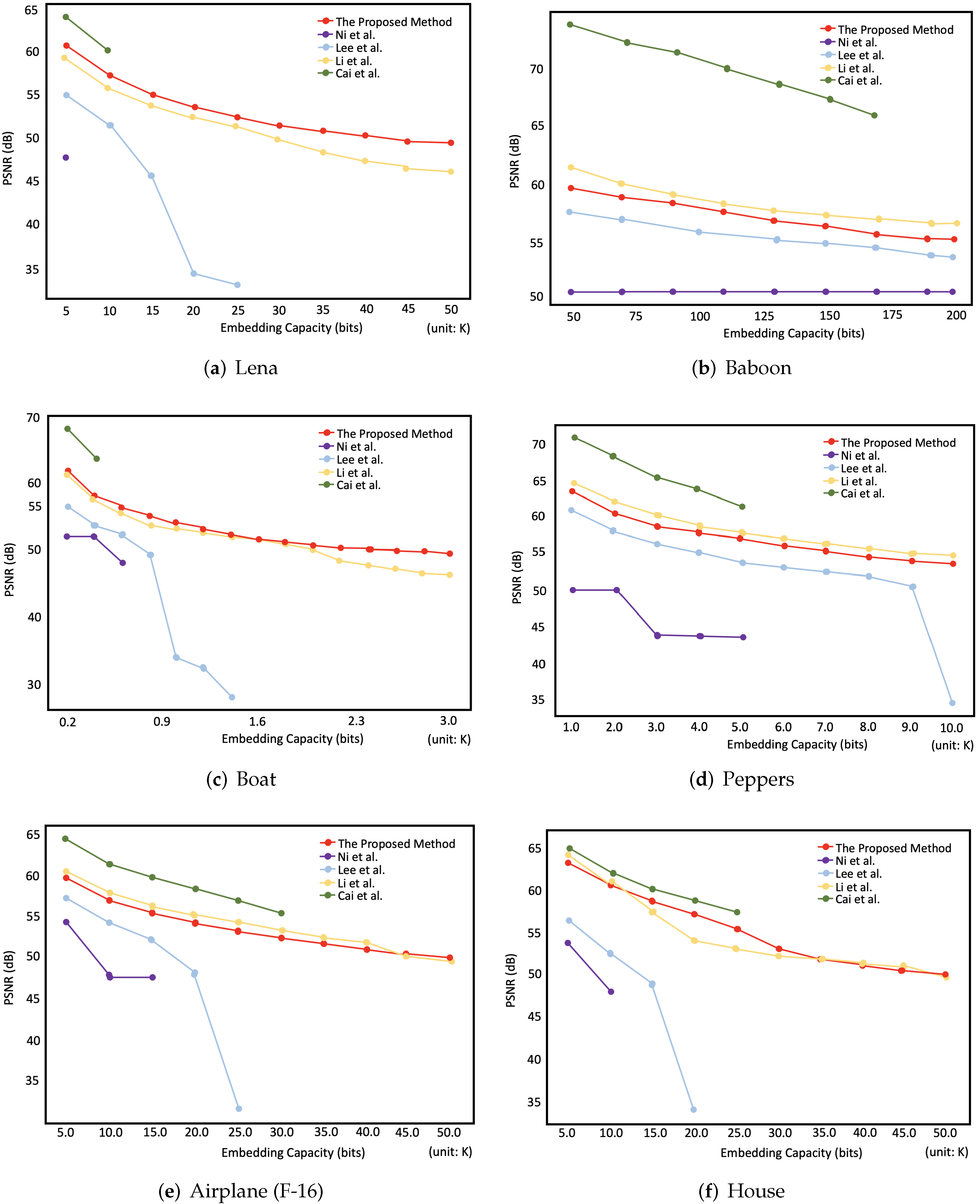
5.1.2. Embedding Capability in Different Embedding Capacities

In this section, the variations in image quality under different embedding capacities between the proposed method and the methods of Ni et al. [46], Lee et al. [47], Li et al. [21], and Cai et al. [5] are compared. The image quality comparison for six test images in different embedding capacities between the proposed method and the other schemes are shown in

Table 11. Comparison of PSNR (dB) between the proposed method and the methods of Ni et al. [46], Lee et al. [47], Li et al. [21], and Cai et al. [5] for a capacity of 1000 bits.

Image	Ni et al.	Lee et al.	Li et al.	Cai et al.	Our Method
Lena	53.75	63.17	66.84	71.30	69.62
Baboon	50.47	55.81	58.59	70.78	57.90
Boat	52.07	60.28	64.63	70.96	64.97
Peppers	50.14	61.14	64.93	70.94	63.61
Aiprplain (F-16)	54.46	63.29	66.68	71.28	66.21
House	54.11	67.52	72.41	72.32	68.51
Average	52.50	61.87	65.68	71.26	65.14

,

Table 12. Comparison of PSNR (dB) between the proposed method and the methods of Ni et al. [46], Lee et al. [47], Li et al. [21], and Cai et al. [5] for a capacity of 5,000 bits.

Image	Ni et al.	Lee et al.	Li et al.	Cai et al.	Our Method
Lena	47.81	55.14	59.50	54.14	60.59
Baboon	44.41	47.23	53.89	–	52.52
Boat	51.99	52.98	56.55	–	57.27
Peppers	44.08	53.96	57.82	61.52	57.00
Airplane (F-16)	54.31	57.34	60.50	64.29	59.86
House	53.98	56.60	64.53	65.28	63.48
Average	49.43	53.88	58.80	63.81	58.45

and

Table 13. Comparison of PSNR (dB) between the proposed method and the methods of Ni et al. [46], Lee et al. [47], Li et al. [21], and Cai et al. [5] for a capacity of 10,000 bits.

Image	Ni et al.	Lee et al.	Li et al.	Cai et al.	Our Method
Lena	–	51.79	55.90	60.32	57.15
Baboon	–	–	50.93	–	50.62
Boat	48.24	46.25	53.35	–	54.00
Peppers	–	48.66	54.53	–	54.11
Airplane (F-16)	48.10	54.47	57.87	61.43	57.18
House	48.35	52.80	61.09	62.25	60.68
Average	48.23	50.79	55.61	61.33	55.62

. In addition, the performance comparisons between the proposed method and other related researches are shown in Figure 8 as line graphs.

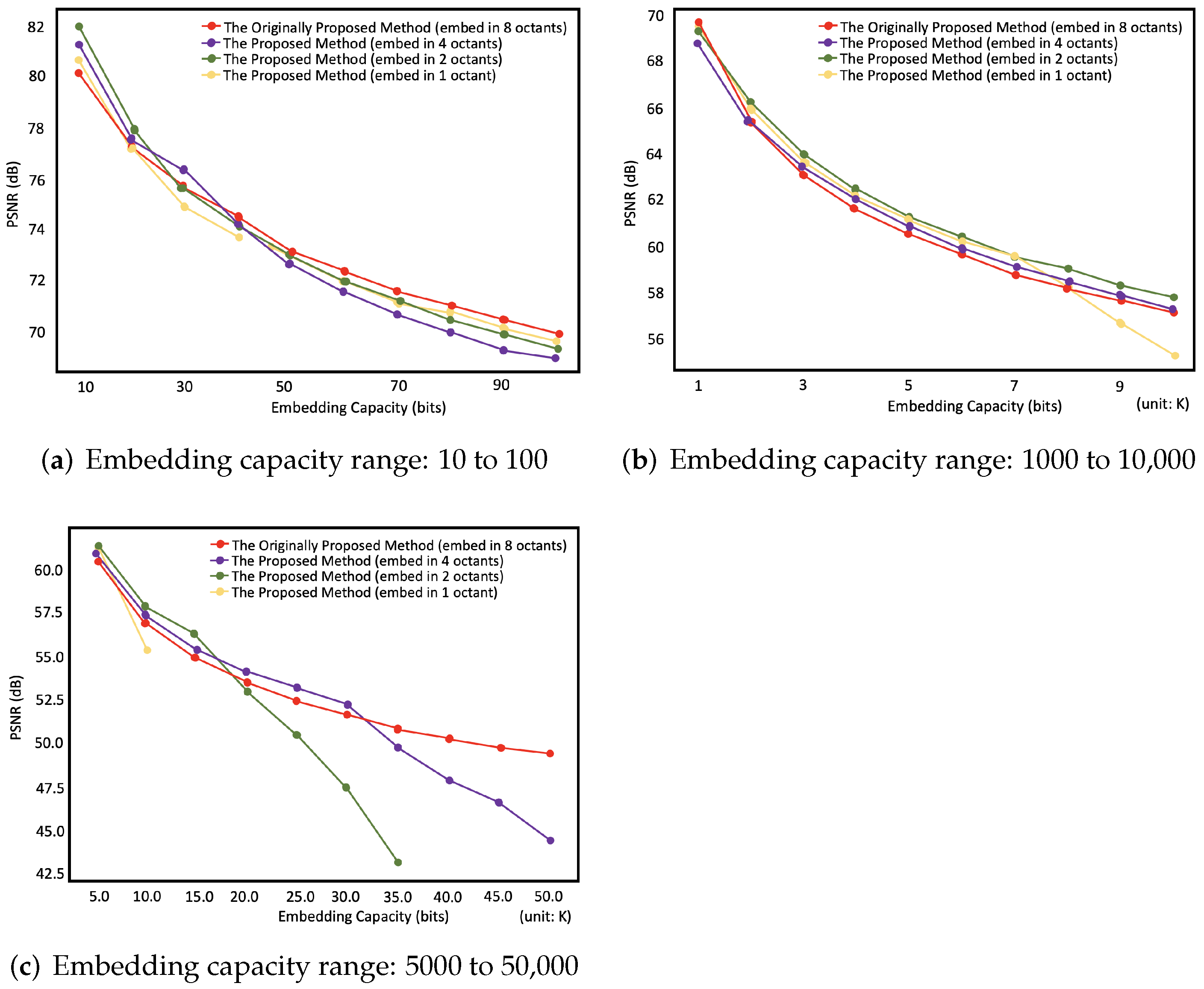
5.2. Comparison between the Proposed Method and the Different Embedding Methods with Different Octant Embed Number

In this subsection, the variations in image quality under different embedding capacities between the proposed method and the different embedding methods are compared. The different embedding methods are generated by reducing the octant embed number of the 3D-PEH in the proposed method. The comparison results are shown in Figure 9.

According to the above results, when the bits of embedded secret data are few, the distortion of the image can be slightly reduced by embedding the secret in fewer octants. Thus, the reducing effect is limited. Conversely, when the bits of embedded secret data is larger, the better quality of the image can be kept by embedding secret in more octants of the 3D-PEH. It can be expected that the more bits of embedded secret data, the larger gap between different embedding methods occurs. Therefore, we consider embedding secret data in eight octants in the proposed method.

6. Conclusions

Machine learning, especially deep learning, has made significant progress in many research areas and applications such as visual recognition, image classification and image processing, etc. However, to the best of our knowledge, no deep learning approaches have been successfully applied to RDH schemes which require images to be completely restored and secret information to be extracted. This motivates us to apply such approaches to RDH. In this paper, we propose a reversible data hiding scheme based on three-dimensional prediction-error histogram modification and MLP networks. We utilize a trained MLP neural network to predict pixel values and combining with PEE to achieve RDH. In addition, the proposed method of modifying the three-dimensional prediction-error histogram can better utilize the space in the three-dimensional coordinates for data embedding. Evaluation of the quality and embedding capacity of the stego-images shows that the proposed method still maintains a good PSNR and increases the maximum embedding capacity which is 1.9–9.8 times of previous methods. Nevertheless, the proposed method still has its disadvantages. Specifically, training the neural network and predicting pixels bit-by-bit are both time-consuming. Developing methods to enhance the efficiency of the proposed method, such as reducing the training time and predicting multiple bits at once, deserves to be further investigated in future works. Moreover, this work focused on proposing a novel reversible data hiding scheme which trains multilayer perceptrons by utilizing the correlation between image pixel values and their adjacent pixels so that the accurate pixel predictions can be achieved. There should be a trade-off between the performance and the fragility. For a future research direction, it is worthy to discuss the impact of fragility caused by transmission errors.

References

1. Yu, J.; Zhang, J. Recent progress on high-speed optical transmission. Digit. Commun. Netw. 2016, 2, 65–76. [Google Scholar] [CrossRef] [Green Version]
2. Wang, C.; Wu, N.; Tsai, C.; Hwang, M. A high quality steganographic method with pixel-value differencing and modulus function. J. Syst. Softw. 2008, 81, 150–158. [Google Scholar] [CrossRef]
3. Alattar, A.M. Reversible watermark using the difference expansion of a generalized integer transformation. IEEE Trans. Image Process. 2004, 13, 1147–1156. [Google Scholar] [CrossRef] [PubMed]
4. Shi, Y.Q. Reversible data hiding. In Proceedings of the International Workshop on Digital Watermarking (IWDW’04), Seoul, Korea, 30 October–1 November 2004; pp. 1–12. [Google Scholar]
5. Cai, S.; Li, X.; Liu, J.; Guo, Z. A new reversible data hiding scheme exploiting high-dimensional prediction-error histogram. In Proceedings of the IEEE International Conference on Image Processing (ICIP’16), Phoenix, AZ, USA, 25–28 September 2016; pp. 2732–2736. [Google Scholar]
6. Shi, Y.Q.; Li, X.; Zhang, X.; Wu, H.T.; Ma, B. Reversible data hiding: Advances in the past two decades. IEEE Access 2016, 4, 3210–3237. [Google Scholar] [CrossRef]
7. Almohammad, A.; Ghinea, G. Stego image quality and the reliability of PSNR. In Proceedings of the 2nd International Conference on Image Processing Theory, Tools and Applications (IPTA’10), Paris, France, 7–10 July 2010; pp. 215–220. [Google Scholar]
8. Thodi, D.M.; Rodriguez, J.J. Expansion embedding techniques for reversible watermarking. IEEE Trans. Image Process. 2007, 16, 721–730. [Google Scholar] [CrossRef] [PubMed]
9. Honga, W.; Chen, T.S.; Shiua, C.W. Reversible data hiding for high quality images using modification of prediction errors. J. Syst. Softw. 2009, 82, 1833–1842. [Google Scholar] [CrossRef]
10. Ou, B.; Li, X.; Zhao, Y.; Ni, R.; Shi, Y.Q. Pairwise prediction-error expansion for efficient reversible data hiding. IEEE Trans. Image Process. 2013, 22, 5010–5021. [Google Scholar] [CrossRef] [PubMed]
11. Caciula, I.; Coltuc, D. Improved control for low bit-rate reversible watermarking. In Proceedings of the IEEE International Conference on Acoustics, Speech and Signal Processing (ICASSP’14), Florence, Italy, 4–9 May 2014; pp. 7425–7429. [Google Scholar]
12. Dragoi, I.C.; Coltuc, D. Local-prediction-based difference expansion reversible watermarking. IEEE Trans. Image Process. 2014, 23, 1779–1790. [Google Scholar] [CrossRef]
13. Dragoi, I.; Coltuc, D. On local prediction based reversible watermarking. IEEE Trans. Image Process. 2015, 24, 1244–1246. [Google Scholar] [CrossRef]
14. Gui, X.; Li, X.; Yang, B. High-dimensional histogram utilization for reversible data hiding. In Proceedings of the International Workshop on Digital Watermarking (IWDW’14), Taipei, Taiwan, 1–4 October 2014; pp. 243–253. [Google Scholar]
15. Hwang, H.J.; Kim, H.J.; Sachnev, V.; Joo, S.H. Reversible watermarking method using optimal histogram pair shifting based on prediction and sorting. KSII Trans. Internet Inf. Syst. 2010, 4, 655–670. [Google Scholar] [CrossRef]
16. Hu, Y.; Lee, H.K.; Li, J. DE-based reversible data hiding with improved overflow location map. IEEE Trans. Circuits Syst. Video Technol. 2008, 19, 250–260. [Google Scholar]
17. Jiang, R.; Zhang, W.; Hou, D.; Wang, H.; Yu, N. Reversible data hiding for 3D mesh models with three-dimensional prediction-error histogram modification. Multimed. Tools Appl. 2018, 77, 5263–5280. [Google Scholar] [CrossRef]
18. Kamstra, L.; Heijmans, H.J.A.M. Reversible data embedding into images using wavelet techniques and sorting. IEEE Trans. Image Process. 2005, 14, 2082–2090. [Google Scholar] [CrossRef]
19. Luo, L.; Chen, Z.; Chen, M.; Zeng, X.; Xiong, Z. Reversible image watermarking using interpolation technique. IEEE Trans. Inf. Forensics Secur. 2009, 5, 187–193. [Google Scholar]
20. Li, X.; Li, J.; Li, B.; Yang, B. High-fidelity reversible data hiding scheme based on pixel-value-ordering and prediction-error expansion. Signal Process. 2013, 93, 198–205. [Google Scholar] [CrossRef]
21. Li, X.; Zhang, W.; Gui, X.; Yang, B. A novel reversible data hiding scheme based on two-dimensional difference-histogram modification. IEEE Trans. Inf. Forensics Secur. 2013, 8, 1091–1110. [Google Scholar]
22. Li, X.; Zhang, W.; Gui, X.; Yang, B. Efficient reversible data hiding based on multiple histograms modification. IEEE Trans. Inf. Forensics Secur. 2015, 10, 2016–2027. [Google Scholar] [CrossRef]
23. Qin, C.; Chang, C.C.; Huang, Y.H.; Liao, L.T. An inpainting-assisted reversible steganographic scheme using a histogram shifting mechanism. IEEE Trans. Circuits Syst. Video Technol. 2012, 23, 1109–1118. [Google Scholar] [CrossRef]
24. Sachnev, V.; Kim, H.J.; Nam, J.; Suresh, S.; Shi, Y.Q. Reversible watermarking algorithm using sorting and prediction. IEEE Trans. Circuits Syst. Video Technol. 2009, 19, 989–999. [Google Scholar] [CrossRef]
25. Xuan, G.; Shi, Y.Q.; Chai, P.; Cui, X.; Ni, Z.C.; Tong, X.F. Optimum histogram pair based image lossless data embedding. In Proceedings of the International Workshop on Digital Watermarking (IWDW’07), Guangzhou, China, 3–5 December 2007; pp. 264–278. [Google Scholar]
26. Xuan, G.; Tong, X.; Teng, J.; Zhang, X.; Shi, Y.Q. Optimal histogram-pair and prediction-error based image reversible data hiding. In Proceedings of the International Workshop on Digital Watermarking (IWDW’12), Shanghai, China, 31 October–3 November 2012; pp. 368–383. [Google Scholar]
27. Wang, J.; Ni, J.; Zhang, X.; Shi, Y.Q. Rate and distortion optimization for reversible data hiding using multiple histogram shifting. IEEE Trans. Cybern. 2016, 47, 315–326. [Google Scholar] [CrossRef]
28. Hornik, K.; Stinchcombe, M.; White, H. Multilayer feedforward networks are universal approximators. Neural Netw. 1989, 2, 359–366. [Google Scholar] [CrossRef]
29. Schalkoff, R.J. Pattern Recognition: Statistical. Structural and Neural Approaches; Wiley: New York, NY, USA, 2007. [Google Scholar]
30. Salgado, C.M.; Dam, R.S.F.; Salgado, W.L.; Werneck, R.R.A.; Pereira, C.M.N.A.; Schirru, R. The comparison of different multilayer perceptron and general regression neural networks for volume fraction prediction using MCNPX code. Appl. Radiat. Isot. 2020, 162, 109170. [Google Scholar] [CrossRef] [PubMed]
31. Sharifzadeh, F.; Akbarizadeh, G.; Kavian, Y.S. Ship classification in SAR images using a new hybrid CNN–MLP classifier. J. Indian Soc. Remote Sens. 2019, 47, 551–562. [Google Scholar] [CrossRef]
32. Heidari, A.A.; Faris, H.; Aljarah, I.; Mirjalili, S. An efficient hybrid multilayer perceptron neural network with grasshopper optimization. Soft Comput. 2019, 23, 7941–7958. [Google Scholar] [CrossRef]
33. Fath, A.H.; Madanifar, F.; Abbasi, M. Implementation of multilayer perceptron (MLP) and radial basis function (RBF) neural networks to predict solution gas-oil ratio of crude oil systems. Petroleum 2020, 6, 80–91. [Google Scholar] [CrossRef]
34. Janani, V.; Maadhuryaa, N.; Pavithra, D.; Sree, S.R. Dengue prediction using (MLP) multilayer perceptron—A machine learning approach. Int. J. Res. Eng. Sci. Manag. 2020, 3, 226–231. [Google Scholar]
35. Fridrich, J.; Goljan, M.; Du, R. Invertible authentication. In Security and Watermarking of Multimedia Contents III; SPIE: Bellingham, WA, USA, 2001; Volume 4314, pp. 197–208. [Google Scholar]
36. Goljan, M.; Fridrich, J.; Du, R. Distortion-free data embedding for images. In Proceedings of the International Workshop on Information Hiding (IHW’01), Pittsburgh, PA, USA, 25–27 April 2001; pp. 27–41. [Google Scholar]
37. Goljan, M.; Fridrich, J.; Du, R. Lossless data embedding: New paradigm in digital watermarking. EURASIP J. Adv. Signal Process. 2002, 2002, 185–196. [Google Scholar]
38. Xuan, G.; Chen, J.; Zhu, J.; Shi, Y.Q.; Ni, Z.; Su, W. Lossless data hiding based on integer wavelet transform. In Proceedings of the IEEE Workshop on Multimedia Signal Processing (MMSP’02), St. Thomas, VI, USA, 9–11 December 2002; pp. 312–315. [Google Scholar]
39. Xuan, G.; Zhu, J.; Chen, J.; Shi, Y.Q.; Ni, Z.; Su, W. Distortionless data hiding based on integer wavelet transform. Electron. Lett. 2002, 38, 1646–1648. [Google Scholar] [CrossRef]
40. Celik, M.U.; Sharma, G.; Tekalp, A.M.; Saber, E. Reversible data hiding. In Proceedings of the IEEE International Conference on Image Processing (ICIP’02), Rochester, NY, USA, 22–25 September 2002; pp. 157–160. [Google Scholar]
41. Celik, M.; Sharma, G.; Tekalp, A.; Saber, E. Lossless generalized-LSB data embedding. IEEE Trans. Image Process. 2005, 14, 253–266. [Google Scholar] [CrossRef] [PubMed]
42. Celik, M.U.; Sharma, G.; Tekalp, A.M. Lossless watermarking for image authentication: A new framework and an implementation. IEEE Trans. Image Process. 2006, 15, 1042–1049. [Google Scholar] [CrossRef] [PubMed]
43. Chang, C.C.; Kieu, T.D. A reversible data hiding scheme using complementary embedding strategy. Inf. Sci. 2010, 180, 3045–3058. [Google Scholar] [CrossRef]
44. Malik, A.; Singh, S.; Kumar, R. Recovery based high capacity reversible data hiding scheme using even-odd embedding. Multimed. Tools Appl. 2018, 77, 15803–15827. [Google Scholar] [CrossRef]
45. Kumar, R.; Chand, S.; Singh, S. A reversible data hiding scheme using pixel location. Int. Arab J. Inf. Technol. 2018, 15, 763–768. [Google Scholar]
46. Ni, Z.; Shi, Y.Q.; Ansari, N.; Su, W. Reversible data hiding. IEEE Trans. Circuits Syst. Video Technol. (TCSVT’06) 2006, 16, 354–362. [Google Scholar]
47. Lee, S.K.; Suh, Y.H.; Ho, Y.S. Reversible image authentication based on watermarking. In Proceedings of the IEEE International Conference on Multimedia and Expo (ICME’06), Toronto, ON, Canada, 9–12 July 2006; pp. 1321–1324. [Google Scholar]
48. Lin, S.J.; Chung, W.H. The scalar scheme for reversible information-embedding in gray-scale signals: Capacity evaluation and code constructions. IEEE Trans. Inf. Forensics Secur. 2012, 7, 1155–1167. [Google Scholar] [CrossRef] [Green Version]
49. Zhang, X. Reversible data hiding with optimal value transfer. IEEE Trans. Multimed. 2012, 15, 316–325. [Google Scholar] [CrossRef]
50. Zhang, W.; Hu, X.; Li, X.; Yu, N. Recursive histogram modification: Establishing equivalency between reversible data hiding and lossless data compression. IEEE Trans. Image Process. 2013, 22, 2775–2785. [Google Scholar] [CrossRef]
51. Zhan, Y.; Su, Y.; Wang, X.; Pei, Q. Three-dimensional prediction-error histograms based reversible data hiding algorithm for color images. Multimed. Tools Appl. 2019, 78, 35289–35311. [Google Scholar] [CrossRef]
52. Kumar, R.; Chand, S.; Singh, S. An improved histogram-shifting-imitated reversible data hiding based on HVS characteristics. Multimed. Tools Appl. 2018, 77, 13445–13457. [Google Scholar] [CrossRef]
53. Wang, Z.H.; Lee, C.F.; Chang, C.Y. Histogram-shifting-imitated reversible data hiding. J. Syst. Softw. 2013, 86, 315–323. [Google Scholar] [CrossRef]
54. Kaur, G.; Singh, S.; Rani, R.; Kumar, R. A comprehensive study of reversible data hiding (RDH) schemes based on pixel value ordering (PVO. Arch. Comput. Methods Eng. 2020, 28, 3517–3568. [Google Scholar] [CrossRef]
55. Kaur, G.; Singh, S.; Rani, R. PVO based reversible data hiding technique for roughly textured images. Multidimens. Syst. Signal Process. 2021, 32, 533–558. [Google Scholar] [CrossRef]
Figure 1. The embedding and extraction frameworks of the spatial domain RDH.
Applsci 12 02502 g001
Figure 2. The flowchart of our method.
Applsci 12 02502 g002
Figure 3. The structure of our MLP neural network.
Applsci 12 02502 g003
Figure 4. (a) Star/dot pixels partition. (b) Scan order for star pixels. (c) Scan order for dot pixels.
Applsci 12 02502 g004
Figure 5. The 3D-PEH mappings for the proposed scheme.
Applsci 12 02502 g005aApplsci 12 02502 g005b
Figure 6. The cover images and the stego-images (embed 10,000 bits).
Applsci 12 02502 g006
Figure 7. PSNR (dB) and embedding capacity (bits) of the proposed scheme, for image Lena.
Applsci 12 02502 g007
Figure 8. Performance comparisons among the proposed method and other approaches on different images.
Applsci 12 02502 g008
Figure 9. PSNR with different embedding methods and capacity ranges for the image Lena.
Applsci 12 02502 g009