
Long-Range Correlations and Natural Time Series Analyses from Acoustic Emission Signals

 , , , , , , and
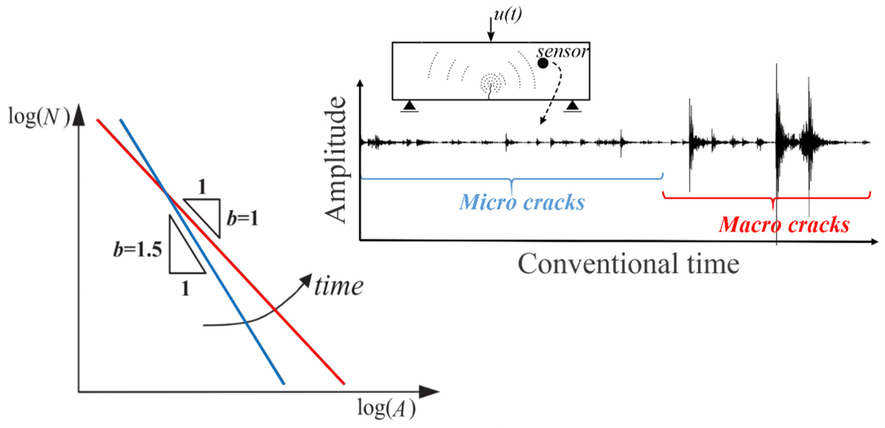
Abstract
:1. Introduction
2. Theoretical Background
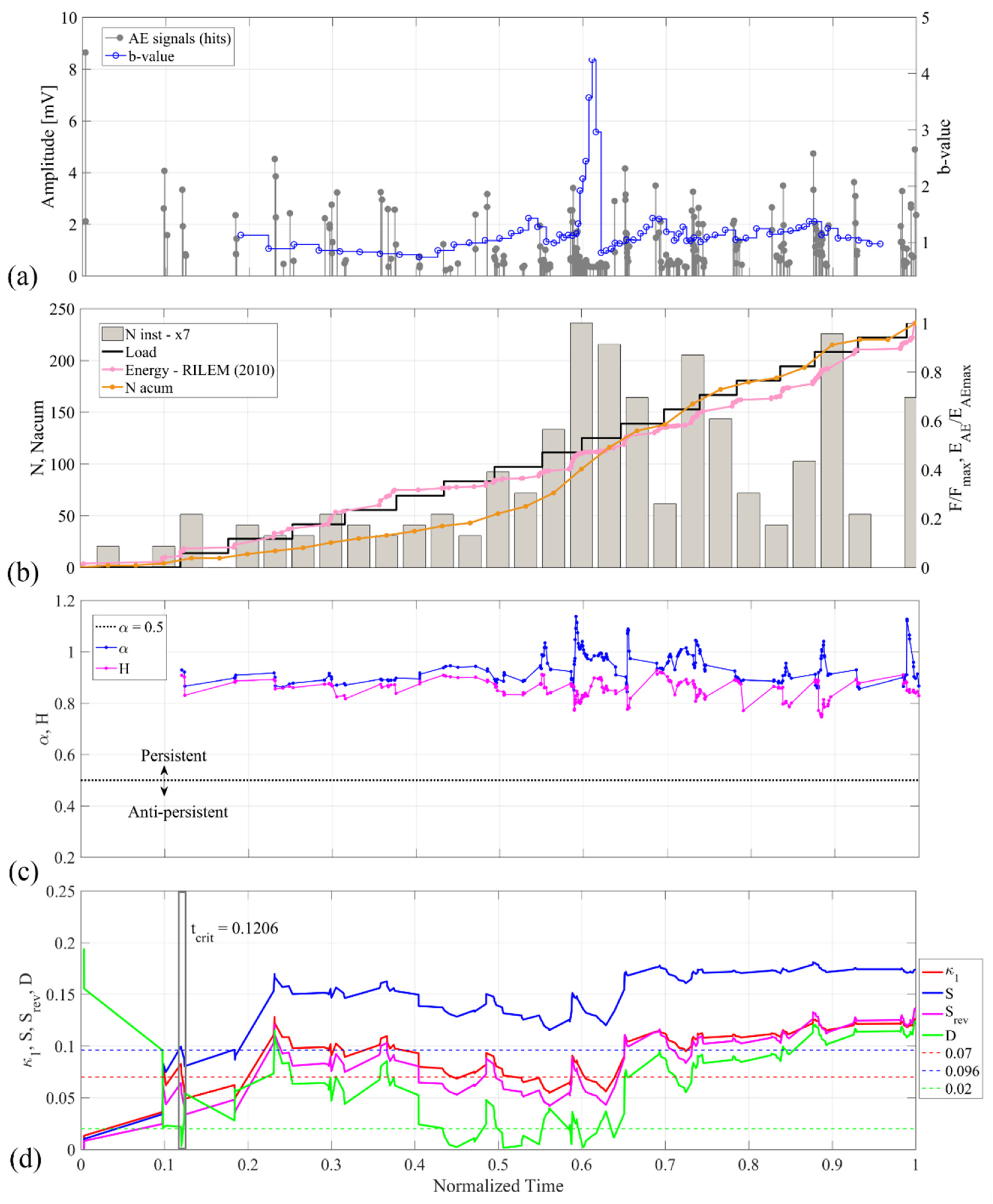
2.1. b-Value Analysis
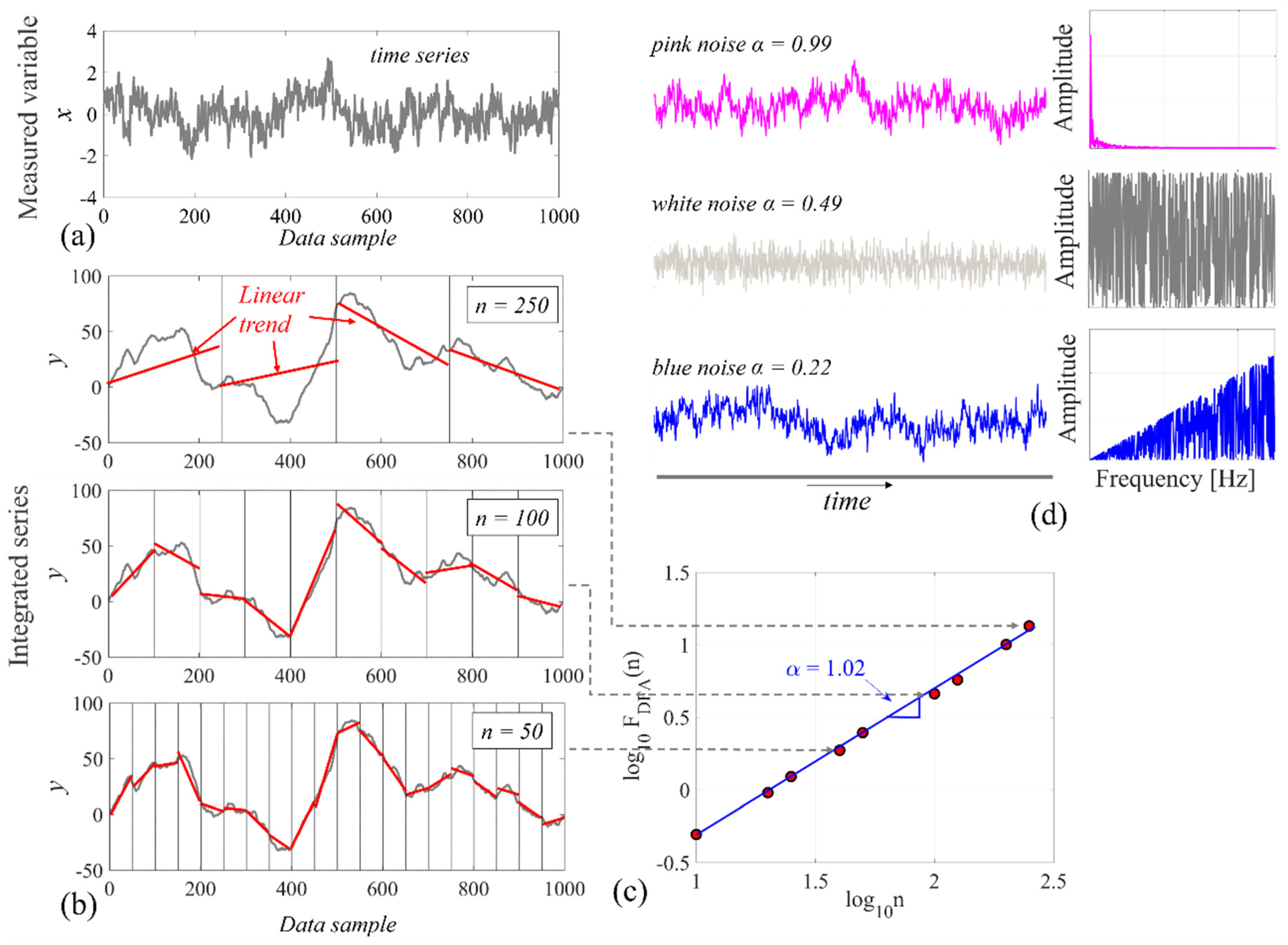
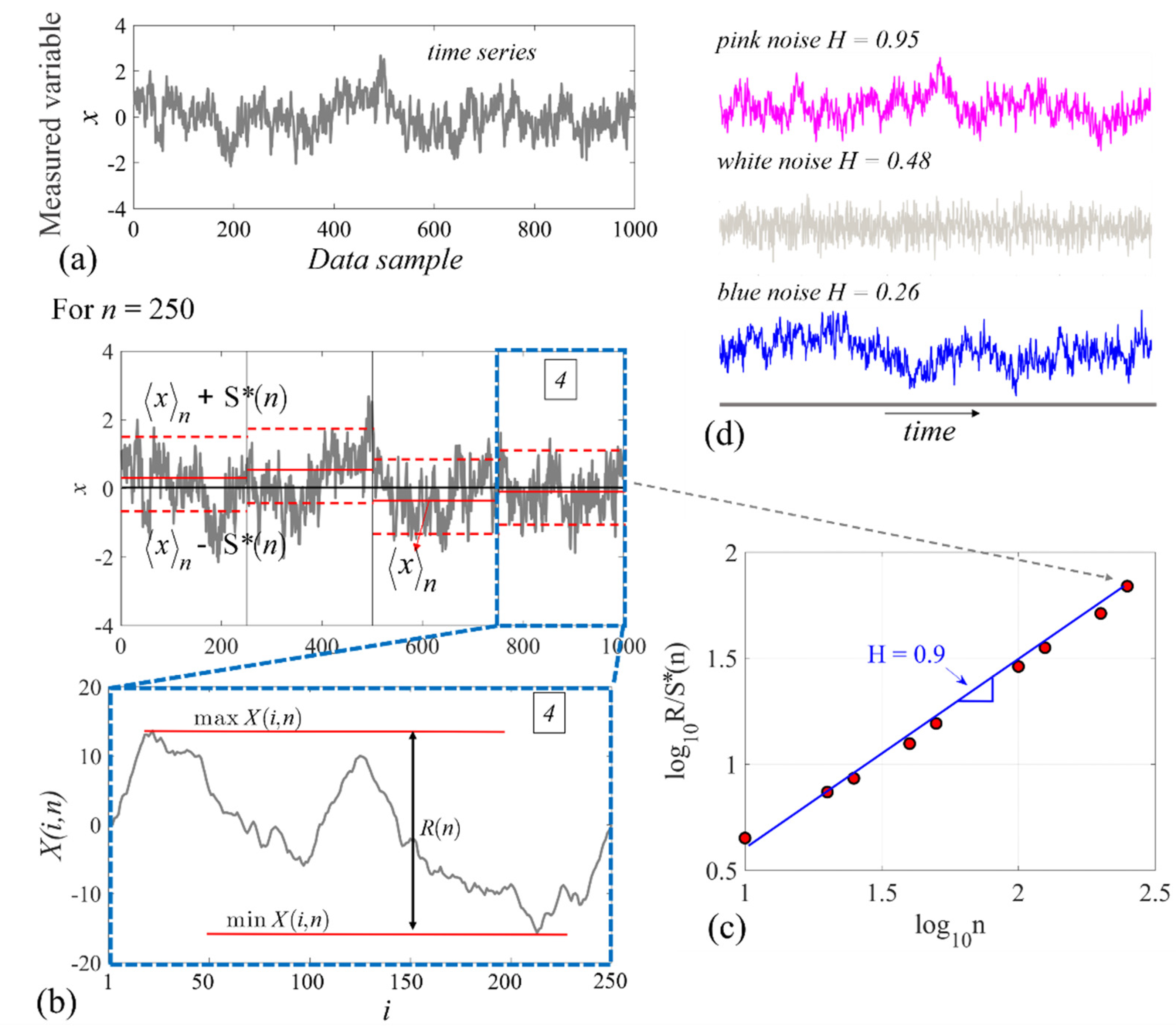
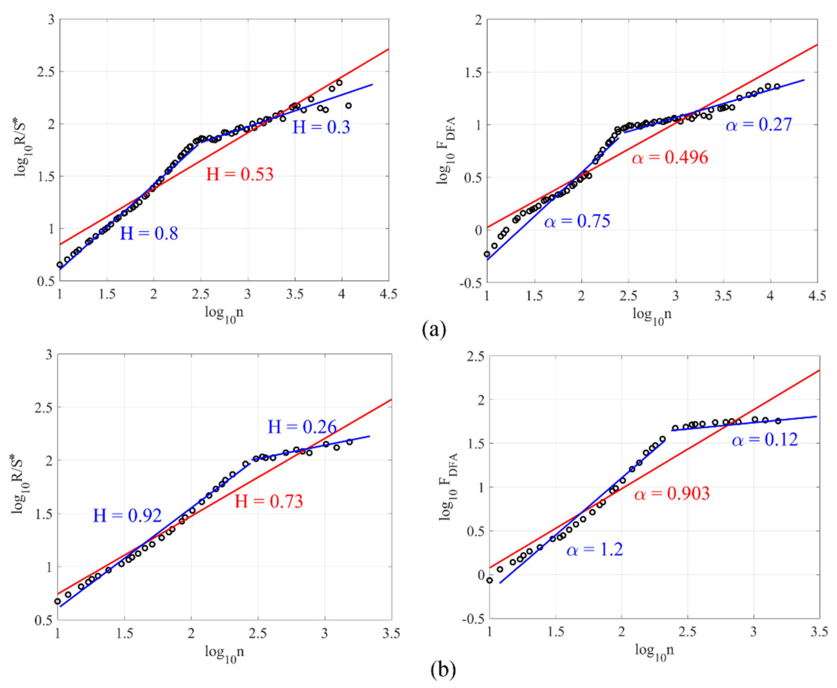
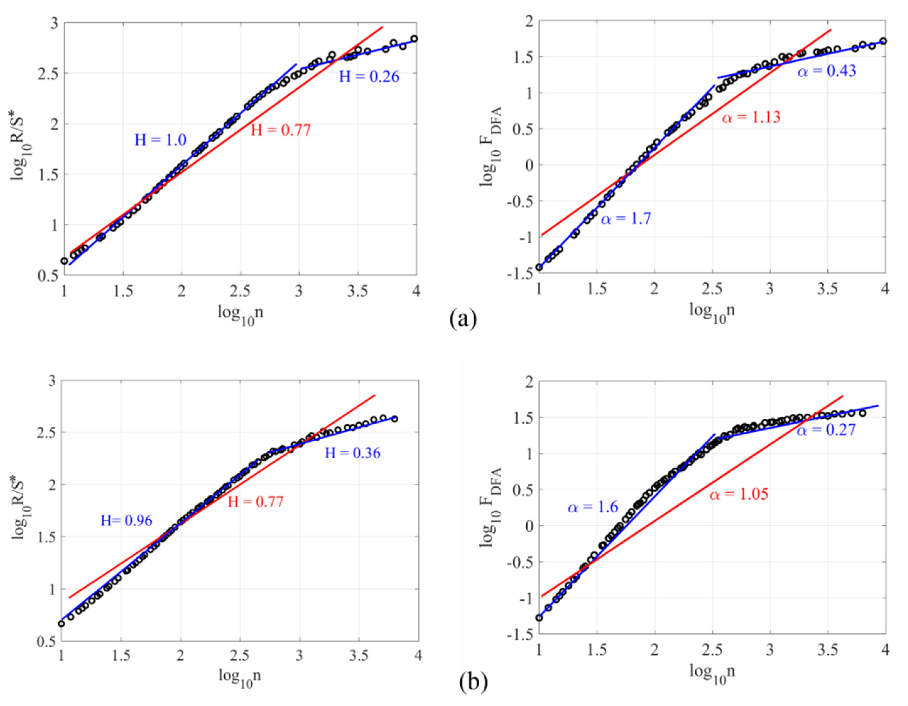
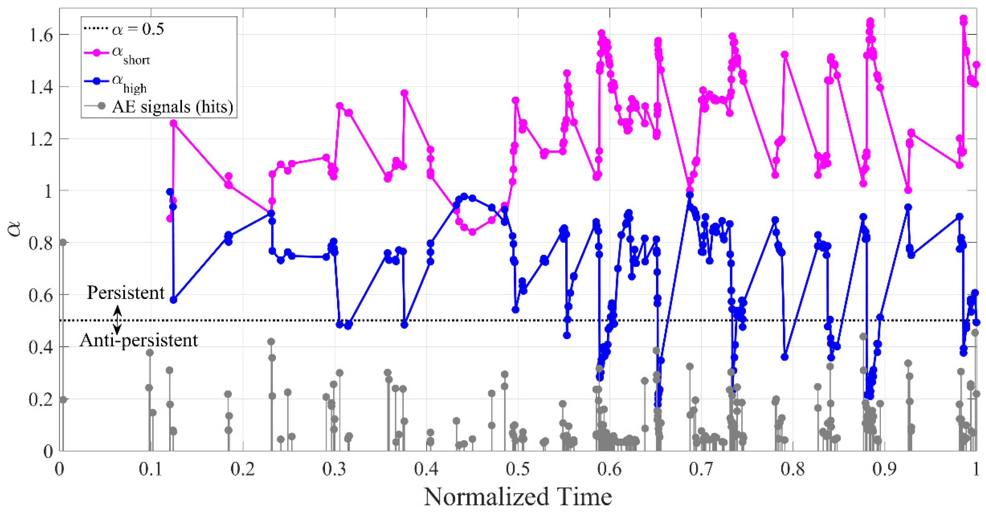
2.2. Long-Range Correlations Measures (DFA and Hurst)
- Integrate the series , obtaining , where and stands for the average of , see Figure 2b.
- Divide into non-overlapping windows of equal length n.
- Calculate the average fluctuation FDFA of the integrated series around the trend series . Explicitly, .
- Repeat step 4 for a broad range of scales (sizes of n) to provide a relationship between FDFA and n, i.e., FDFA(n).
- Plot log FDFA(n) versus log(n) (see Figure 2c). If there is an obvious linear relationship between them, the slope of its least-squares fit estimates the scaling exponent .
- Take the mean of the n-th window, marked as the solid red lines in Figure 3b.
- Sum the differences from the mean to get the cumulative total at each data point, from the beginning of the period to any desired point, i.e., , Figure 3b.
- Calculate the local range as the maximum fluctuation of the sum of the deviation from the mean, where and are the maximum and minimum values of , respectively, and (Figure 3b).
- Take the standard deviation over the window to normalize the range relative to the input fluctuations in the series (dashed red lines in Figure 3b).
- Rescale the range, that is, calculate .
- Finally, calculate the mean value of the rescaled range for all windows, nw (four in the case of Figure 3b):
- Although this work is focused only on first-order fitting functions, as suggested in [43], higher-order fitting curves can also be used.
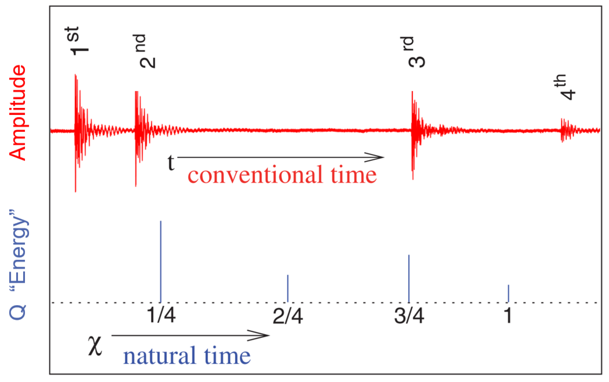
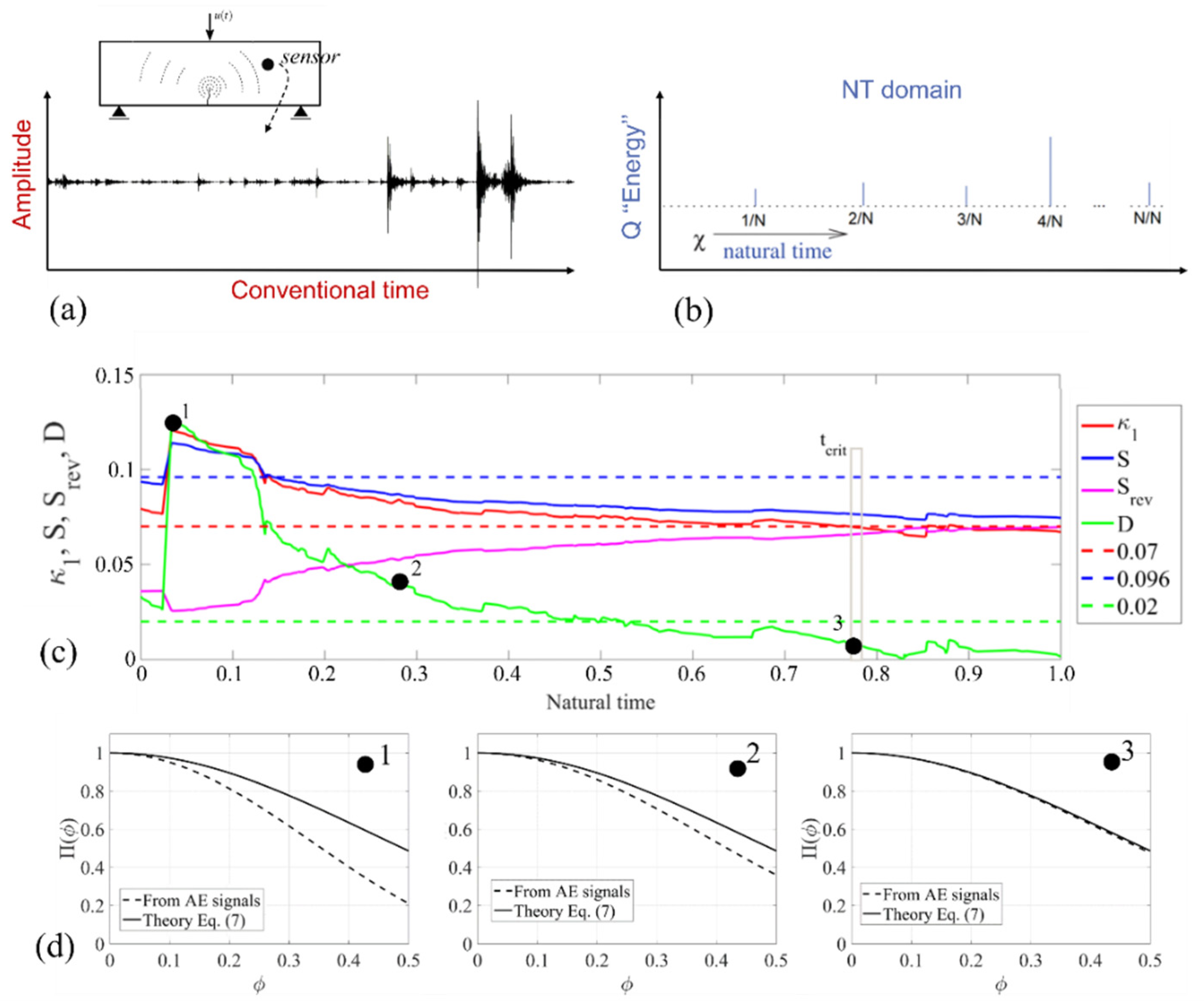
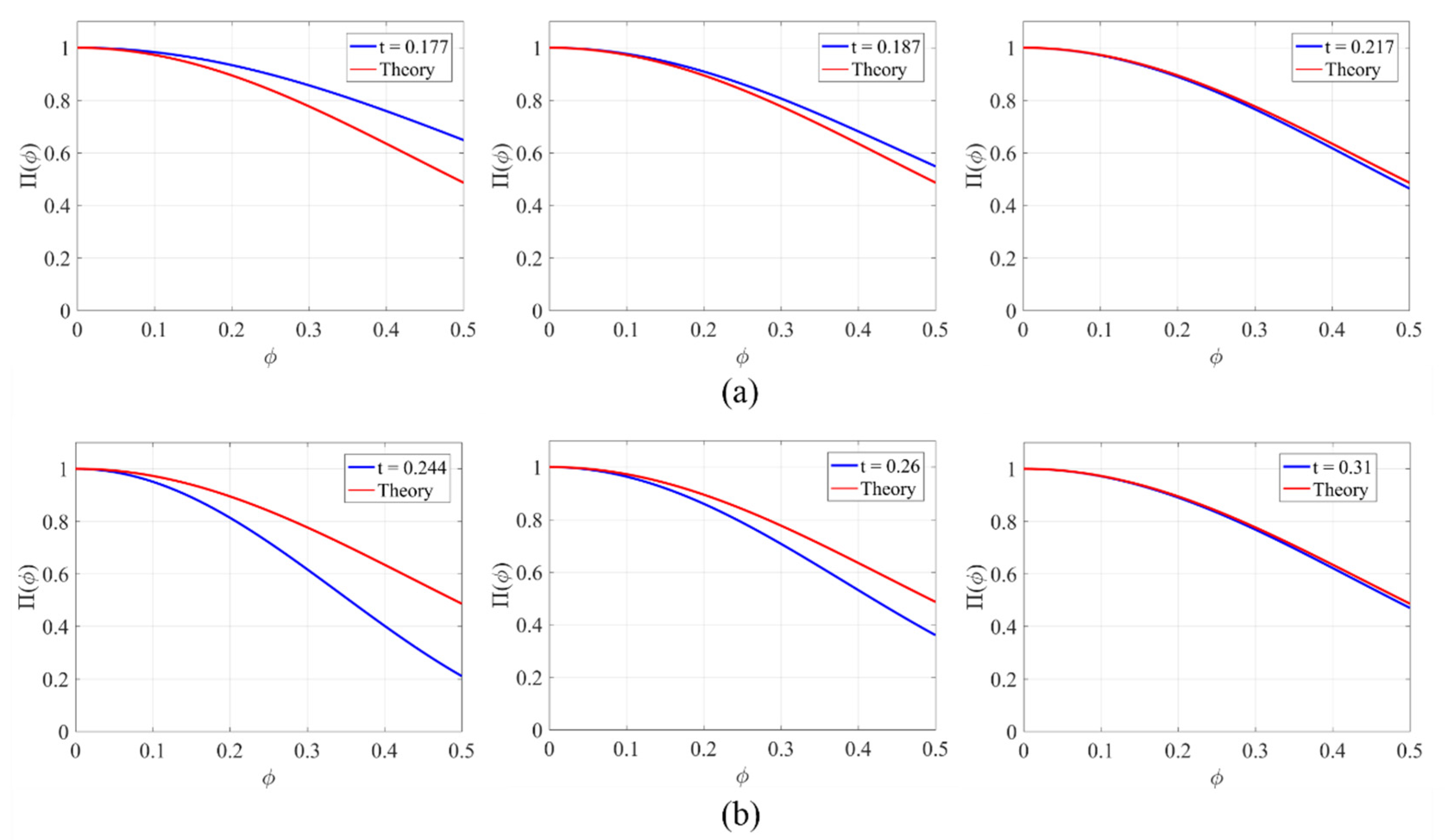
2.3. Natural-Time Analysis
- The “average” distance becomes smaller than 10−2.
- The variance , when descending from above, approaches 0.070;
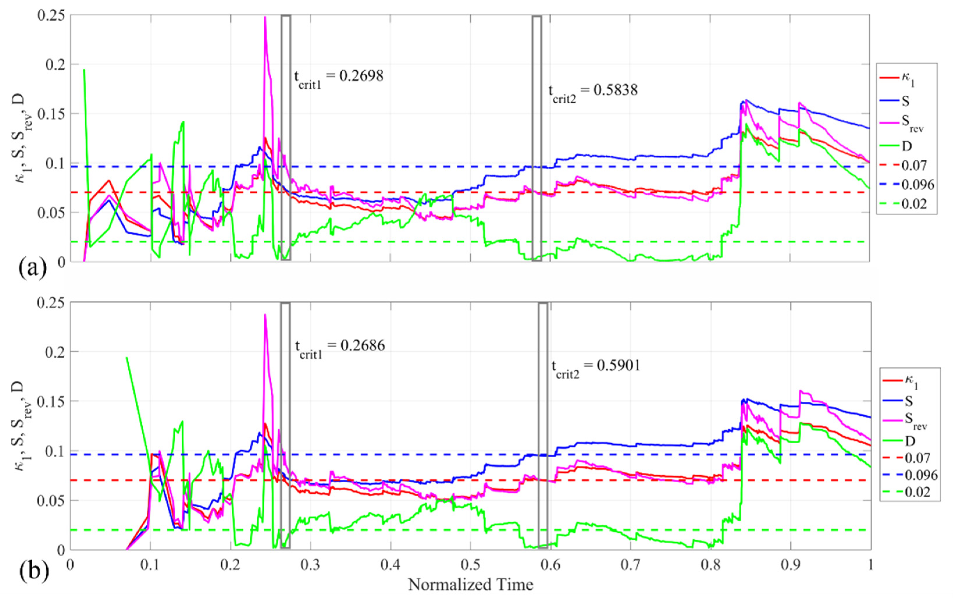
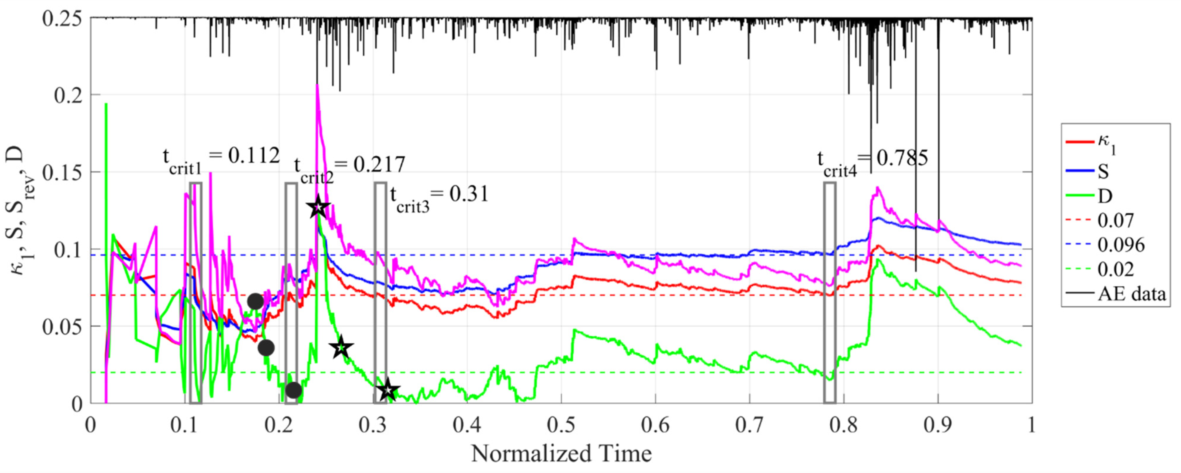
3. Applications
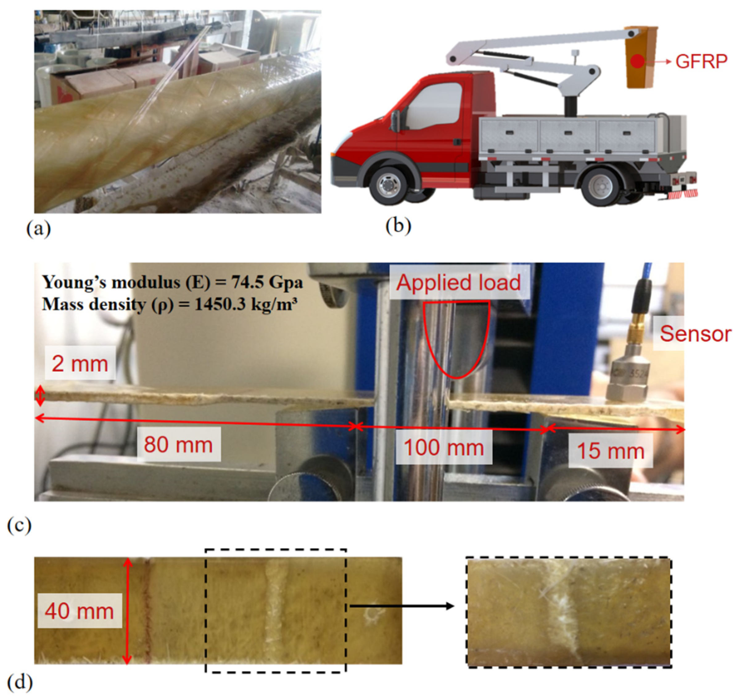
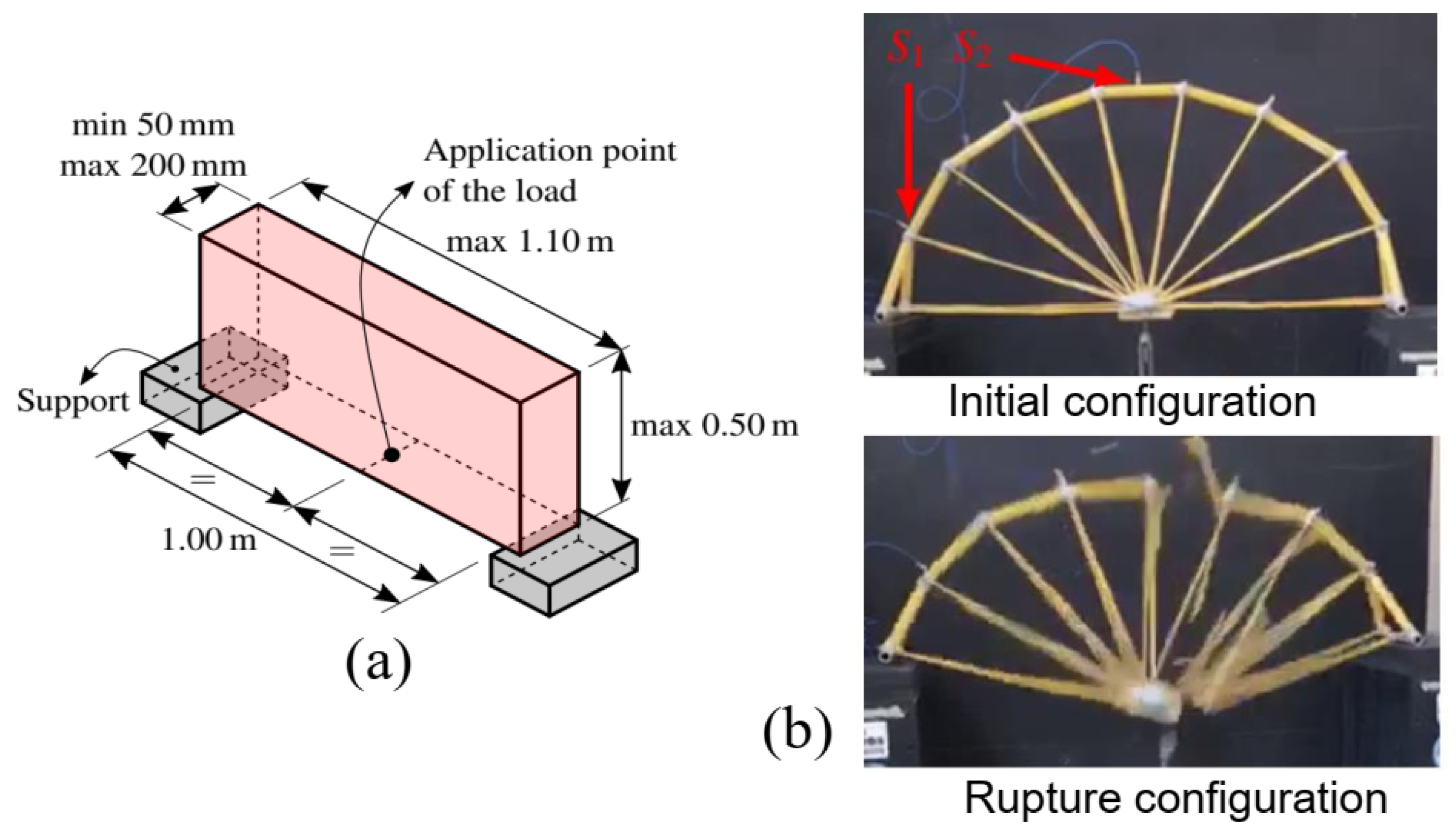
3.1. Three-Point Bending Test of a Glass Fiber-Reinforced Polymeric Plate
3.1.1. Test Description
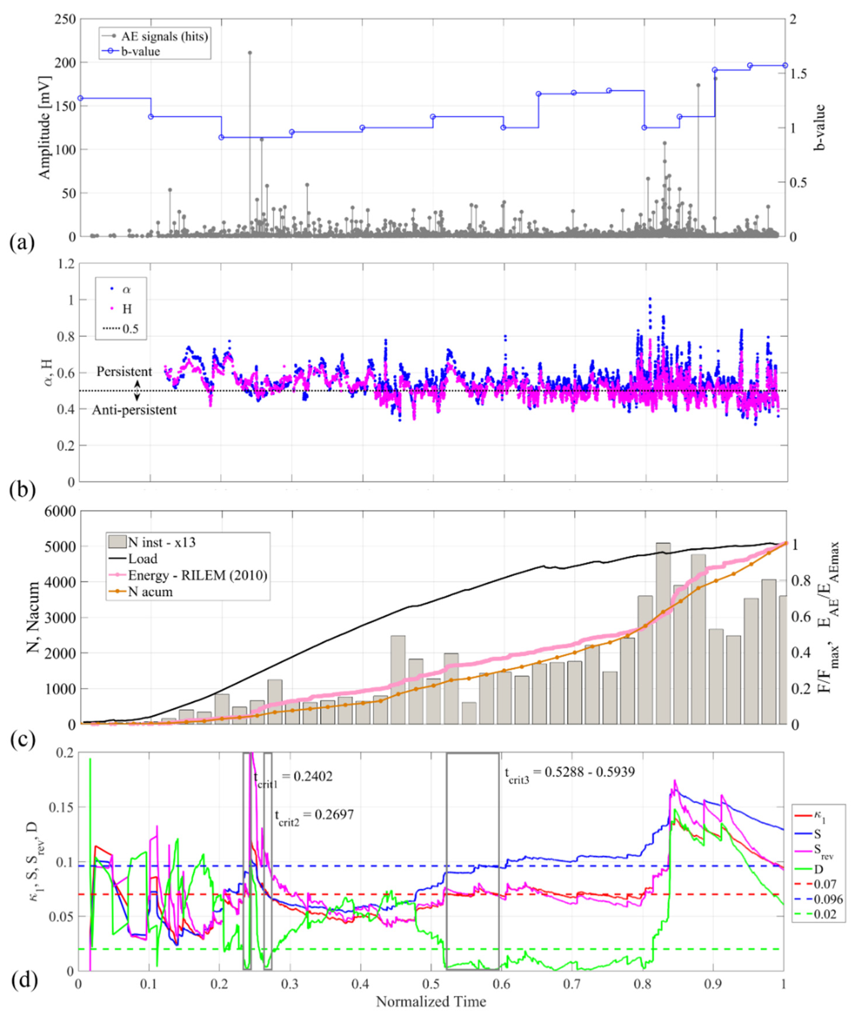
3.1.2. Results
3.1.3. Discussion
3.2. “Spaghetti” Bridge Model
3.2.1. Test Description
3.2.2. Results
3.2.3. Discussion
4. Conclusions
- Both the Hurst and DFA exponents yielded very similar results, which indicate that no high-order trends are present in the data.
- For both applications, the DFA parameter that was calculated for the whole dataset was inconclusive. However, when considered separately, the low () and high () state levels indicated a critical region where one converged to extreme anti-persistent correlations, and the other, to extreme persistent ones. That highlights these parameters’ usefulness in indicating the criticality of the structure.
- The analysis in the natural time domain showed that the convergence of the order parameters and the entropies could predict the structure’s entry in a critical stage, whether it is calculated from the AE energy or from counting the ruptured samples.
- The indexes that were analyzed here, among others used the b-value which led to identifying when the damage process approaches a critical regime. In this situation, an unstable behavior is imminent and it is characterized by an increment in the global AE activity and in the amplitude of the AE signals. However, it is worth pointing out that it may also happen that, after reaching a critical phase with a large emission of energy, if the conditions of the damage continue to evolve in the structure, another stable one follows, which can be followed by another critical one, etc. Therefore, reaching a critical phase can always be correlated with local instability, but it is not always necessarily correlated with global structural failure. See, e.g., Ref. [14].
Author Contributions
Funding
Institutional Review Board Statement
Informed Consent Statement
Acknowledgments
Conflicts of Interest
Nomenclature
| N | Cumulative number of events/hits |
| A | Signal amplitude |
| Amax | Maximum signal amplitude |
| b | b-value parameter |
| D, d | Fractal dimension |
| FDFA | Average fluctuations in DFA |
| n | Window size |
| α | Angular coefficient of log FDFA x log n |
| Nmax | Total number of points in the series |
| x | A time series |
| y | Integrate the time series |
| X | Sum the differences from the mean in Hurst analysis |
| R | Local range |
| S* | Standard deviation |
| nw | Total number of windows |
| H | Hurst exponent |
| nmin | Smallest window size |
| nmax | Largest window size |
| χ | Natural time |
| Q | Energy of the individual event |
| p | Normalized energy (Q) |
| κ1 | Natural time χ’s variance |
| S | Entropy in natural time |
| Srev | Time-reversal entropy |
| <D> | “Average” distance |
| ω | Natural angular frequency |
| ϕ | Frequency in natural time |
| Π | Normalized power spectrum |
| Su | Entropy of uniform noise |
| E | Young’s modulus |
| p | Mass density |
| αshort | Short-term windows |
| αhigh | Long-term windows |
References
- Nemat-Nasser, S.; Hori, M. Micromechanics: Overall Properties of Heterogeneous Materials (North-Holland Series in Applied Mathematics and Mechanics); Elsevier: Amsterdam, The Netherlands, 1999. [Google Scholar]
- Torquato, S. Random Heterogeneous Materials: Microstructure and Macroscopic Properties; Springer: New York, NY, USA, 2013. [Google Scholar]
- Gross, D.; Seelig, T. Fracture Mechanics—With an Introduction to Micromechanics; Mechanical Engineering Series; Springer: Berlin/Heidelberg, Germany, 2006. [Google Scholar]
- Kachanov, L. Time of the rupture process under creep conditions. Izvestiia Akademii Nauk SSSR 1957, 8, 26–31. [Google Scholar]
- Chaboche, J. Continuum damage mechanics: Present state and future trends. Nucl. Eng. Des. 1987, 105, 19–33. [Google Scholar] [CrossRef]
- Voyiadjuis, G.Z. Handbook of Damage Mechanics, Nano to Macro Scale for Materials and Structures; Springer: Berlin/Heidelberg, Germany, 2014. [Google Scholar]
- Daniels, H.E. The statistical theory of the strength of bundles of threads I. Proc. R. Soc. Lond. 1945, 183, 405–435. [Google Scholar]
- Hansen, A.; Hemmer, P.C.; Pradhan, S. The Fiber Bundle Model: Modeling Failure in Materials (Statistical Physics of Fracture and Breakdown); Wiley-VCH Verlag GmbH & Co. KGaA: Weinheim, Germany, 2015; ISBN 978-3-527-41214-3. [Google Scholar]
- Jenabidehkordi, A. Computational methods for fracture in rock: A review and recent advances. Front. Struct. Civ. Eng. 2019, 13, 273–287. [Google Scholar] [CrossRef]
- Grosse, C.U.; Ohtsu, M. Acoustic Emission Testing; Springer: Berlin/Heidelberg, Germany, 2008. [Google Scholar]
- Aki, K. Scaling law of seismic spectrum. J. Geophys. Res. 1967, 72, 1217–1231. [Google Scholar] [CrossRef]
- Carpinteri, A.; Lacidogna, G.; Puzzi, S. From criticality to final collapse: Evolution of the b-value from 1.5 to 1.0. Chaos Solitons Fractals 2009, 41, 843–853. [Google Scholar] [CrossRef]
- Carpinteri, A.; Lacidogna, G.; Accornero, F. Fluctuations of 1/f Noise in Damaging Structures Analyzed by Acoustic Emission. Appl. Sci. 2018, 8, 1685. [Google Scholar] [CrossRef] [Green Version]
- Carpinteri, A.; Lacidogna, G.; Corrado, M.; Di Battista, E. Cracking and Crackling in Concrete-Like Materials: A Dynamic Energy Balance. Eng. Fract. Mech. 2016, 155, 130–144. [Google Scholar] [CrossRef]
- Alava, M.J.; Nukala, P.K.V.V.; Zapperi, S. Statistical models of fracture. Adv. Phys. 2006, 55, 349–476. [Google Scholar] [CrossRef] [Green Version]
- Xu, D.; Liu, P.; Chen, Z.; Cai, Q.; Leng, J. Dynamic feature evaluation on streaming acoustic emission data for adhesively bonded joints for composite wind turbine blade. Struct. Health Monit. 2021. [Google Scholar] [CrossRef]
- Wilson, K.G. Problems in Physics with Many Scales of Length. Sci. Am. 1979, 241, 140–157. [Google Scholar] [CrossRef]
- Tainter, J.A. The Collapse of Complex Societies, New Studies in Archaeology; Cambridge University Press: Cambridge, UK, 1988; ISBN 978-0-521-38673-9. [Google Scholar]
- Rosser, J.B. The Rise and Fall of Catastrophe Theory Applications in Economics: Was the Baby Thrown Out with the Bathwater. J. Econ. Dyn. Control. 2007, 31, 3255–3280. [Google Scholar] [CrossRef]
- Rundle, J.B.; Turcotte, D.L.; Shcherbakov, R.; Klein, W.; Sammis, C. Statistical physics approach to understanding the multiscale dynamics of earthquake fault systems. Rev. Geophys. 2003, 41, 1019–1041. [Google Scholar] [CrossRef] [Green Version]
- Turcotte, D.L.; Newman, W.I.; Shcherbakov, R. Micro and Macroscopic Models of Rock Fracture. Geophys. J. Int. 2003, 152, 718–728. [Google Scholar] [CrossRef] [Green Version]
- Hurst, H.E. Long-term storage capacity of reservoirs. Trans. Am. Soc. Civ. Eng. 1951, 116, 770–808. [Google Scholar] [CrossRef]
- Peng, C.K.; Buldyrev, S.V.; Havlin, S.; Simons, M.; Stanley, H.E.; Goldberger, A.L. Mosaic Organization of DNA Nucleotides. Phys. Rev. E 1994, 49, 1685–1689. [Google Scholar] [CrossRef] [Green Version]
- Varotsos, P.A.; Sarlis, N.V.; Skordas, E.S. Spatio-temporal complexity aspects on the interrelation between seismic electric signals and seismicity. Pract. Athens Acad. 2001, 76, 294–321. [Google Scholar]
- Potirakis, S.M.; Karadimitrakis, A.; Eftaxias, K. Natural time analysis of critical phenomena: The case of pre-fracture electromagnetic emissions. Chaos 2013, 23, 023117. [Google Scholar] [CrossRef]
- Friedrich, L.; Colpo, A.; Maggi, A.; Becker, T.; Lacidogna, G.; Iturrioz, I. Damage process in glass fiber reinforced polymer specimens using acoustic emission technique with low frequency acquisition. Compos. Struct. 2021, 256, 113105. [Google Scholar] [CrossRef]
- Tanzi, R.B.N.; Sobczyk, M.; Becker, T.; González, L.A.S.; Vantadori, S.; Iturrioz, I.; Lacidogna, G. Damage Evolution Analysis in a “Spaghetti” Bridge Model Using the Acoustic Emission Technique. Appl. Sci. 2021, 11, 2718. [Google Scholar] [CrossRef]
- Sagasta, F.; Zitto, M.E.; Piotrkowski, R.; Benavent-Climent, A.; Suarez, E.; Gallego, A. Acoustic emission energy b-value for local damage evaluation in reinforced concrete structures subjected to seismic loadings. Mech. Syst. Signal Processing 2018, 102, 262–277. [Google Scholar] [CrossRef]
- Richter, C.F. Elementary Seismology; W. H. Freeman and Company: London, UK, 1958. [Google Scholar]
- Carpinteri, A.; Lacidogna, G.; Niccolini, G. Fractal analysis of damage detected in concrete structural elements under loading. Chaos Solitons Fractals 2009, 42, 2047–2056. [Google Scholar] [CrossRef]
- Varotsos, P.A.; Sarlis, N.V.; Skordas, E.S. Detrended fluctuation analysis of the magnetic and electric field variations that precede rupture. Chaos Interdiscip. J. Nonlinear Sci. 2009, 19, 023114. [Google Scholar] [CrossRef] [PubMed] [Green Version]
- Kantelhardt, J.W.; Koscielny-Bunde, E.; Rego, H.H.A.; Havlin, S.; Bunde, A. Detecting long-range correlations with detrended fluctuation analysis. Phys. A Stat. Mech. Its Appl. 2001, 295, 441–454. [Google Scholar] [CrossRef] [Green Version]
- Mandelbrot, B.B. The Fractal Geometry of Nature; W. H. Freeman and Company: New York, NY, USA, 1982. [Google Scholar]
- Filho, A.M.; da Silva, M.F.; Zebende, G.F. Autocorrelation and cross-correlation in time series of homicide and attempted homicide. Phys. A Stat. Mech. Its Appl. 2014, 400, 12–19. [Google Scholar] [CrossRef] [Green Version]
- Coronado, A.V.; Carpena, P. Size Effects on Correlation Measures. J. Biol. Phys. 2005, 31, 121–133. [Google Scholar] [CrossRef] [Green Version]
- Talkner, P.; Weber, R.O. Power spectrum and detrended fluctuation analysis: Application to daily temperatures. Phys. Rev. E 2000, 62, 150–160. [Google Scholar] [CrossRef] [Green Version]
- Rigoli, L.M.; Lorenz, T.; Coey, C.; Kallen, R.; Jordan, S.; Richardson, M.J. Co-actors Exhibit Similarity in Their Structure of Behavioural Variation That Remains Stable Across Range of Naturalistic Activities. Sci. Rep. 2020, 10, 6308. [Google Scholar] [CrossRef] [Green Version]
- Hu, K.; Ivanov, P.C.; Chen, Z.; Carpena, P.; Stanley, H.E. Effect of trends on detrended fluctuation analysis. Phys. Rev. E Stat. Nonlin. Soft. Matter. Phys. 2001, 64, 011114. [Google Scholar] [CrossRef] [Green Version]
- Landa, E.; Morales, I.O.; Fossion, R.; Stránský, P.; Velázquez, V.; Vieyra, J.C.L.; Frank, A. Criticality and long-range correlations in time series in classical and quantum systems. Phys. Rev. E 2011, 84, 016224. [Google Scholar] [CrossRef]
- Damouras, S.; Chang, M.D.; Sejdić, E.; Chau, E. An empirical examination of detrended fluctuation analysis for gait data. Gait Posture 2010, 31, 336–340. [Google Scholar] [CrossRef] [PubMed]
- Mariani, M.C.; Asante, P.K.; Bhuiyan, M.A.M.; Beccar-Varela, M.P.; Jaroszewicz, S.; Tweneboah, O.K. Long-Range Correlations and Characterization of Financial and Volcanic Time Series. Mathematics 2020, 8, 441. [Google Scholar] [CrossRef] [Green Version]
- Bassingthwaighte, J.B.; Raymond, G.M. Evaluating rescaled range analysis for time series. Ann. Biomed. Eng. 1994, 22, 432–444. [Google Scholar] [CrossRef] [PubMed]
- Li, J.; Chen, Y. Rescaled range (R/S) analysis on seismic activity parameters. Acta Seismol. Sin. 2001, 14, 148–155. [Google Scholar] [CrossRef]
- Varotsos, P.A.; Sarlis, N.V.; Skordas, E.S. Long-range correlations in the electric signals that precede rupture. Phys. Rev. E 2002, 66, 011902. [Google Scholar] [CrossRef] [PubMed] [Green Version]
- Hausdorff, J.M.; Mitchell, S.L.; Firtion, R.; Peng, C.-K.; Cudkowitz, M.E.; Wei, J.Y.; Goldberger, A.L. Altered fractal dynamics of gait: Reduced stride-interval correlations with aging and Huntington’s disease. J. Appl. Physiol. 1997, 82, 262–269. [Google Scholar] [CrossRef]
- Jordan, K.; Challis, J.H.; Newell, K.M. Long range correlations in the stride interval of running. Gait Posture 2006, 24, 120–125. [Google Scholar] [CrossRef]
- Niccolini, G.; Manuello, A.; Marchis, E.; Carpinteri, A. Signal frequency distribution and natural-time analysis from acoustic emission monitoring of an arched structure in the Castle of Racconigi. Nat. Hazards Earth Syst. Sci. 2017, 1025–1032. [Google Scholar] [CrossRef] [Green Version]
- Varotsos, P.A.; Panayiotis, A.; Sarlis, N.V.; Skordas, E.S. Natural Time Analysis: The New View of Time; Springer: Berlin/Heidelberg, Germany, 2011. [Google Scholar] [CrossRef]
- Loukidis, A.; Perez-Oregon, J.; Pasiou, E.D.; Sarlis, N.V.; Triantis, D. Similarity of fluctuations in critical systems: Acoustic emissions observed before fracture. Phys. A Stat. Mech. Appl. 2021, 566, 125622. [Google Scholar] [CrossRef]
- Ramírez-Rojas, A.; Flores-Márquez, E.L. Order parameter analysis of seismicity of the Mexican Pacific coast. Phys. A Stat. Mech. Appl. 2013, 392, 2507–2512. [Google Scholar] [CrossRef]
- Shannon, C.E. A mathematical theory of communication. Bell Syst. Tech. J. 1948, 27, 379–423. [Google Scholar] [CrossRef] [Green Version]
- Potirakis, S.M.; Mastrogiannis, D. Critical features revealed in acoustic and electromagnetic emissions during fracture experiments on LiF. Phys. A Stat. Mech. Appl. 2017, 485, 11–12. [Google Scholar] [CrossRef]
- Daniel, S.H. Seismic electric signals (SES) and earthquakes: A review of an updated VAN method and competing hypotheses for SES generation and earthquake triggering. Phys. Earth Planet. Inter. 2020, 302, 106484. [Google Scholar]
- Varotsos, P.A.; Panayiotis, A.; Sarlis, N.V.; Skordas, E.S. Long-range correlations in the electric signals that precede rupture: Further investigations. Phys. Rev. E 2003, 67, 021109. [Google Scholar] [CrossRef] [Green Version]
- Varotsos, P.A.; Tanaka, H.K.; Sarlis, N.V.; Skordas, E.S. Similarity of fluctuations in correlated systems: The case of seismicity. Phys. Rev. E 2005, 72, 041103. [Google Scholar] [CrossRef] [Green Version]
- Varotsos, P.A.; Sarlis, N.V.; Skordas, E.S.; Tanaka, H.K.; Lazaridou, M.S. Attempt to distinguish long-range temporal correlations from the statistics of the increments by natural time analysis. Phys. Rev. E 2006, 74, 021123. [Google Scholar] [CrossRef]
- Niccolini, G.; Potirakis, S.M.; Lacidogna, G.; Borla, O. Criticality Hidden in Acoustic Emissions and in Changing Electrical Resistance during Fracture of Rocks and Cement-Based Materials. Materials 2020, 13, 5608. [Google Scholar] [CrossRef]
- Akovali, G. Handbook of Composite Fabrication; Rapra Tech Ltd.: Shrewsbury, UK, 2001. [Google Scholar]
- Imap. Available online: https://imap.com.br (accessed on 20 March 2020).
- RILEM Technical Committee. Recommendation of RILEM TC 212-ACD: Acoustic emission and related NDE techniques for crack detection and damage evaluation in concrete: Test method for classification of active cracks in concrete structures by acoustic emission. Mater. Struct. 2010, 43, 1187–1189. [Google Scholar]
- Skordas, E.S.; Christopoulos, S.R.G.; Sarlis, N.V. Detrended fluctuation analysis of seismicity and order parameter fluctuations before the M7.1 Ridgecrest earthquake. Nat. Hazards 2020, 100, 697–711. [Google Scholar] [CrossRef]
- Carpinteri, A.; Niccolini, G.; Lacidogna, G. Time Series Analysis of Acoustic Emissions in the Asinelli Tower during Local Seismic Activity. Appl. Sci. 2018, 8, 1012. [Google Scholar] [CrossRef] [Green Version]
- Kanamori, H.; Anderson, D.L. Theoretical basis of some empirical relationships in seismology. Bull. Seismol. Soc. Am. 1975, 65, 1073–1095. [Google Scholar]
- Hloupis, G.; Stavrakas, I.; Pasiou, E.D.; Triantis, D.; Kourkoulis, S.K. Natural Time Analysis of Acoustic Emissions in Double Edge Notched Tension (DENT) Marble Specimens. Procedia Eng. 2015, 109, 248–256. [Google Scholar] [CrossRef] [Green Version]
- Hloupis, G.; Stavrakas, I.; Vallianatos, F.; Triantis, D. A preliminary study for prefailure indicators in acoustic emissions using wavelets and natural time analysis. Proc. Inst. Mech. Eng. Part L J. Mater. Des. Appl. 2016, 230, 780–788. [Google Scholar] [CrossRef]
- Lin, A.-J.; Shang, P.-J.; Zhou, H.-C. Effects of Exponential Trends on Correlations of Stock Markets. Math. Probl. Eng. 2014, 2014, 340845. [Google Scholar] [CrossRef] [Green Version]
- Silva, F.E.; Gonçalves, L.L.; Fereira, D.B.B.; Rebello, J.M.A. Characterization of failure mechanism in composite materials through fractal analysis of acoustic emission signals. Chaos Solitons Fractals 2005, 26, 481–494. [Google Scholar] [CrossRef] [Green Version]
- Loukidis, A.; Pasiou, E.D.; Sarlis, N.V.; Triantis, D. Fracture analysis of typical construction materials in natural time. Phys. A Stat. Mech. Appl. 2020, 547, 123831. [Google Scholar] [CrossRef]
- González, S.L.A.; Morsch, I.B.; Masuero, J.R. Didactic Games in Engineering Teaching—Case: Spaghetti Bridges Design and Building Contest. In Proceedings of the 18th International Congress of Mechanical Engineering (COBEM 2005), Ouro Preto, MG, Brazil, 6–11 November 2005. [Google Scholar]


Publisher’s Note: MDPI stays neutral with regard to jurisdictional claims in published maps and institutional affiliations. |
© 2022 by the authors. Licensee MDPI, Basel, Switzerland. This article is an open access article distributed under the terms and conditions of the Creative Commons Attribution (CC BY) license (https://creativecommons.org/licenses/by/4.0/).
Share and Cite
Friedrich, L.F.; Cezar, É.S.; Colpo, A.B.; Tanzi, B.N.R.; Sobczyk, M.; Lacidogna, G.; Niccolini, G.; Kosteski, L.E.; Iturrioz, I. Long-Range Correlations and Natural Time Series Analyses from Acoustic Emission Signals. Appl. Sci. 2022, 12, 1980. https://doi.org/10.3390/app12041980
Friedrich LF, Cezar ÉS, Colpo AB, Tanzi BNR, Sobczyk M, Lacidogna G, Niccolini G, Kosteski LE, Iturrioz I. Long-Range Correlations and Natural Time Series Analyses from Acoustic Emission Signals. Applied Sciences. 2022; 12(4):1980. https://doi.org/10.3390/app12041980
Chicago/Turabian StyleFriedrich, Leandro Ferreira, Édiblu Silva Cezar, Angélica Bordin Colpo, Boris Nahuel Rojo Tanzi, Mario Sobczyk, Giuseppe Lacidogna, Gianni Niccolini, Luis Eduardo Kosteski, and Ignacio Iturrioz. 2022. "Long-Range Correlations and Natural Time Series Analyses from Acoustic Emission Signals" Applied Sciences 12, no. 4: 1980. https://doi.org/10.3390/app12041980