Article

Data-Driven Approach to Modeling Biohydrogen Production from Biodiesel Production Waste: Effect of Activation Functions on Model Configurations

by
SK Safdar Hossain
1,*,
Bamidele Victor Ayodele
2,3,*,
Zaid Abdulhamid Alhulaybi
1 and
Muhammad Mudassir Ahmad Alwi
4
1
Department of Chemical Engineering, College of Engineering, King Faisal University, P.O. Box 380, Al-Ahsa 31982, Saudi Arabia
2
Department of Chemical Engineering, Universiti Teknologi PETRONAS, Seri Iskandar 32610, Perak, Malaysia
3
Center of Contaminant Control & Utilization (CenCou), Institute of Contaminant Management for Oil and Gas, Universiti Teknologi PETRONAS, Seri Iskandar 32610, Perak, Malaysia
4
Department of Materials Engineering, College of Engineering, King Faisal University, P.O. Box 380, Al-Ahsa 31982, Saudi Arabia
*
Authors to whom correspondence should be addressed.
Appl. Sci. 2022, 12(24), 12914; https://doi.org/10.3390/app122412914
Submission received: 9 November 2022 / Revised: 4 December 2022 / Accepted: 13 December 2022 / Published: 15 December 2022

Abstract

:

Featured Application

This study explored the feasibility of various multilayer perceptron configurations for modeling biohydrogen production from biodiesel production waste. Based on the best model, knowledge of how various parameters influence biohydrogen production can be employed in designing an optimized bioreactor that could maximize production processes.

Abstract

Biodiesel production often results in the production of a significant amount of waste glycerol. Through various technological processes, waste glycerol can be sustainably utilized for the production of value-added products such as hydrogen. One such process used for waste glycerol conversion is the bioprocess, whereby thermophilic microorganisms are utilized. However, due to the complex mechanism of the bioprocess, it is uncertain how various input parameters are interrelated with biohydrogen production. In this study, a data-driven machine-learning approach is employed to model the prediction of biohydrogen from waste glycerol. Twelve configurations consisting of the multilayer perceptron neural network (MLPNN) and the radial basis function neural network (RBFNN) were investigated. The effect of using different combinations of activation functions such as hyperbolic tangent, identity, and sigmoid on the model’s performance was investigated. Moreover, the effect of two optimization algorithms, scaled conjugate gradient and gradient descent, on the model performance was also investigated. The performance analysis of the models revealed that the manner in which the activation functions are combined in the hidden and outer layers significantly influences the performance of various models. Similarly, the model performance was also influenced by the nature of the optimization algorithms. The MLPNN models displayed better predictive performance compared to the RBFNN models. The RBFNN model with softmax as the hidden layer activation function and identity as the outer layer activation function has the least predictive performance, as indicated by an R2 of 0.403 and a RMSE of 301.55. While the MLPNN configuration with the hyperbolic tangent as the hidden layer activation function and the sigmoid as the outer layer activation function yielded the best performance as indicated by an R2 of 0.978 and a RMSE of 9.91. The gradient descent optimization algorithm was observed to help improve the model’s performance. All the input variables significantly influence the predicted biohydrogen. However, waste glycerol has the most significant effects.

1. Introduction

The quest for energy transition to a carbon-neutral economy has increased strategies to end all fossil fuel-related carbon emissions by the middle of the 21st century [1]. Reducing energy-related carbon dioxide (CO2) emissions is a top priority in the struggle against global warming [2]. More efforts are being made towards the realization of cutting carbon emissions and alleviating the consequences of climate change [3,4,5]. Nevertheless, the energy industry must be decarbonized in order to achieve the set target. To achieve the carbon neutrality target, renewable energy initiatives have been reported to play a vital role and have the potential to provide up to 90% of the required carbon reductions [1,6]. In view of these renewable energy sources such as, solar, wind, hydro, tidal, geothermal, and biomass, have been extensively explored and reported to have a significant contribution towards attaining carbon neutrality in the future [7,8].
Among the various renewable energy sources, biomass has been reported to have great potential to facilitate the actualization of the carbon neutrality target [9]. According to a recent report, if present agricultural practices underwent the anticipated improvements, 1 billion dry tonnes of biomass may be available for energy use per year [10]. That will amount to approximately 14 quadrillion British thermal units annually by 2030. Therefore, biomass has been projected as an important source of sustainable energy in the future [11]. From biomass resources, liquid biofuels like bioethanol and biodiesel can be produced [12]. Besides, the by-product (or waste) from biomass processing can be sustainably utilized to produce value-added products such as hydrogen. The primary byproduct of biodiesel processing is glycerol, with yields of around 10% (w/w) [13]. Consequently, around 1.05 pounds of glycerol are generated for every gallon of biodiesel, which could be a huge source of hydrogen production.
An extensive review by Schwengber et al. [14] revealed that hydrogen can be produced from glycerol through different technological pathways such as steam reforming, partial oxidation reforming, auto thermal reforming, aqueous phase reforming, and supercritical water reforming. Some of these processes are energy-intensive and facilitate catalyst deactivation by sintering and carbon deposition. Alternatively, a non-energy-intensive process can be employed to produce hydrogen from glycerol. This process involves the use of thermophilic microorganisms to directly convert glycerol to hydrogen. However, one of the drawbacks of this process is the influence of media compositions on thermophilic biohydrogen production from waste glycerol. To overcome this challenge, authors such as Sittijunda and Reungsang [15] employed a response surface optimization strategy to optimize the process parameters in order to maximize biohydrogen production. Although optimum conditions were obtained for biohydrogen production, it is uncertain to what extent each of the parameters influence biohydrogen production. This uncertainty can be attributed to the complex bioreaction mechanisms from the conversion of glycerol to the formation of hydrogen. This puzzle can be solved using a data-driven modeling approach by employing machine learning algorithms such as an artificial neural network.
Different types of machine-learning algorithms have been employed to model various processes involving hydrogen production. Hossain et al. [16] employed Gaussian process regression to model bioethanol production from fountain grass. The findings revealed that an optimized Gaussian process regression successfully modeled the prediction of bioethanol production from fountain grass with an R2 of 0.993. The pH of the medium was reported to have a significant influence on bioethanol production. In comparison to the support vector machine regression, the Gaussian process regression was found to have a better performance when employed to model hydrogen production from waste effluent from bioprocesses. Machine learning algorithms are also robust in evaluating the interaction of process parameters and their effect on the process output, as reported by Hossain et al. [17]. However, a comparative analysis of different machine learning algorithms for modeling hydrogen production by co-gasification of biomass and coal revealed that the artificial neural network (ANN) algorithm offers superior performance. To the best of the authors’ knowledge, the application of multilayer perceptron and radial basis function neural networks as well as the effect of activation functions on the network configuration for modeling the prediction of biohydrogen from biodiesel production waste has not been reported in the literature. Based on these premises, this study focuses on the application of different architectures of multilayer perceptron neural networks in comparison with selected radial basis function neural networks for the modeling of biohydrogen production from biodiesel production waste, with a particular focus on the effect of activation functions on model configurations.

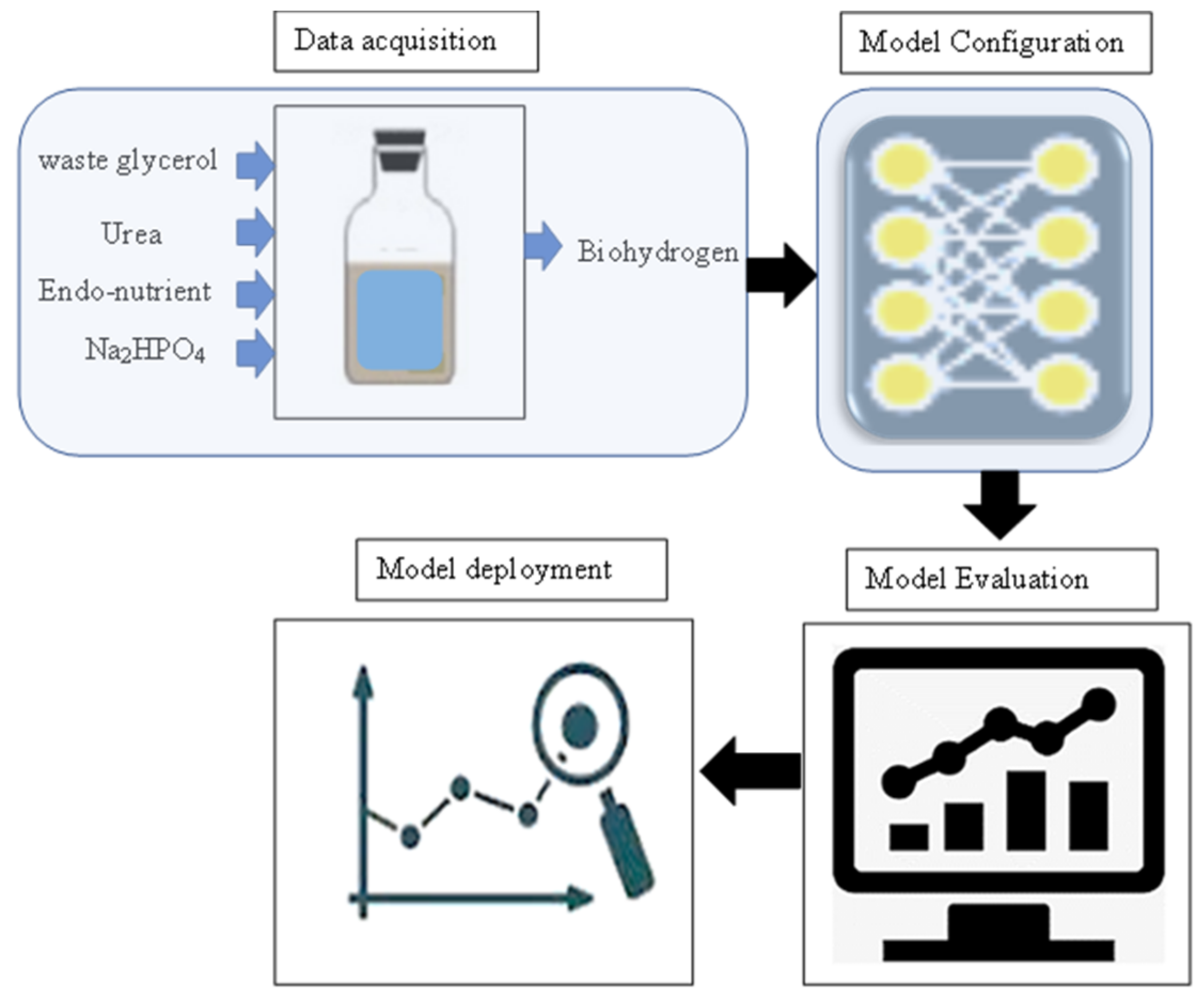
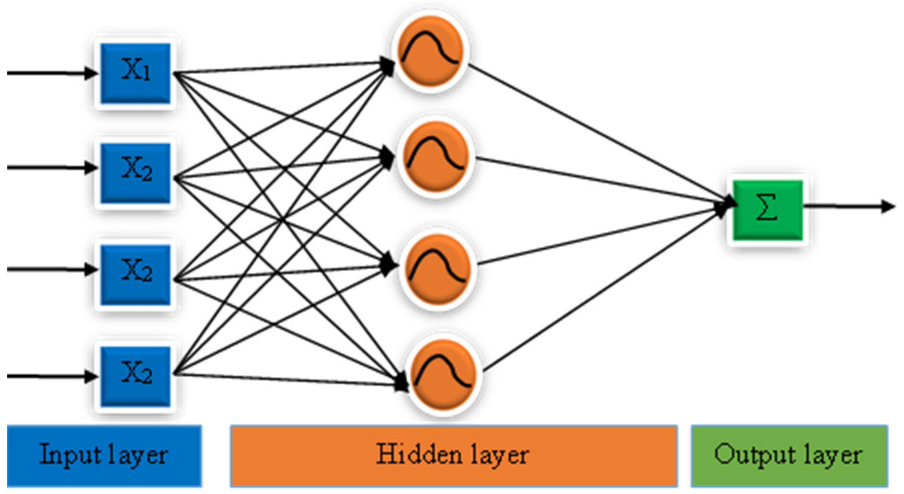
2. Experimental and Model Configuration

The overall process flow for the modeling of biohydrogen production from waste glycerol is depicted in Figure 1. Typically, there are four stages for the prediction of biohydrogen production namely: data acquisition, model configuration, model evaluation, and model deployment.
The data acquisition stage involved experiments on biohydrogen production. In the experimental batch run, waste glycerol was utilized as the substrate. The experimental runs were performed in a 100-mL serum bottle as described by Sittijunda and Reungsang [15]. The fermentation medium in the serum bottle consisted of waste glycerol, urea, Na2HPO4, Endo-nutrient, and inoculum. According to the design, the concentrations of each medium element were changed. The experiment was designed to investigate the effect of Urea Endo-nutrient, Na2HPO4, and the amount of waste glycerol per liter of the medium on biohydrogen production. Experimental data consisting of 29 runs in batch mode, was employed for training various models used in this study.
In the configuration stage, a multilayer perceptron neural network, denoted MLPNN, and a radial basis function neural network, denoted RBFNN (Figure 2), were employed. The MLPNN is a form of feed-forward neural network configured to achieve optimal performance [18]. The network configuration consists of three distinct types of layers, which include an input layer, an output layer, and a hidden layer [19]. The signal to be processed was brought into the system at the input layer. While the output layer facilitated the prediction of the targeted parameters. In an MLPNN, the true computational engine was comprised of an arbitrary number of interconnected hidden layers that were located between the input and output layers [20]. An MLPNN functions similarly to a feed-forward network in that data flows forward from the input layer to the output layer [21]. The neurons of the MLPNN were often trained using a technique known as backpropagation learning [22]. Since MLPNNs were designed to be able to approximate any continuous function, they may be able to tackle problems that cannot be separated linearly. Typically, the configuration of the MLPNN consisted of three steps namely: variable selection, partitioning of the datasets for training and testing, and architecture specification. In step 1, the variables (both dependent and independent) were selected and loaded into the IBM Neural Network Modeller (IBM SPSS Version 22 environment). The datasets were subsequently partitioned in such a way that 70% was used for training and 30% for testing. The activation function for the hidden and outer layers was subsequently selected. This was important because how successfully the network model learns the training dataset will depend on the activation function that was used for the hidden layer. The kind of predictions the model can produce will depend on the activation function that is used for the output layer. Therefore, the activation function for any neural network model must be carefully selected. The effect of combining various activation functions on the model’s performance was investigated. The activation functions investigated included hyperbolic, sigmoid, and identity functions. Scaled conjugate gradient and gradient descent were employed as the optimization algorithms for training. The learning rate of the model, which controls how much the weights are adjusted at each update, was initially set at 0.1. The learning rate changed as the training proceeded for the MLPNN, whereas the values remained unchanged for the RBFNN. The learning rate reduction, in epochs, was set to 10, which is the number of epochs of the training sample required to reduce the initial learning rate to its lower boundary. A detailed description of the various configurations of the MLPNN is summarized in Table 1.
The RBFNN, whose architecture was a form of feed-forward neural network that was robust in addressing issues with function [23], universal approximation and quicker learning pace of RBFNN set them apart from other neural networks. The RBFNN consisted of the input layer, the hidden layer, and the output layer [24]. Similar to the MLPNN, the RBFNN configuration involved the selection of a variable, the partitioning of the dataset, and the setting of the architecture. The dataset was split into two proportions for: training (70%) and testing (30%). During the training, once the computed error reaches the appropriate values or the required number of training iterations has been reached, the RBFNN model’s training will be stopped. Two configurations of the RBFNN, which utilized the ordinary radial basis activation function and the standard radial basis activation function, were employed in this study. Equation (1) was used to determine the output of the ith activation function in the hidden layer of the network as a function of the distance between the input vectors and the center [25].
i ( x c i ) = exp ( x c i 2 2 σ j 2 )
where the symbol ‖ ‖ denotes the Euclidean norms, ci denotes the center of the hidden neurons, σ denotes the width of the hidden neuron [26].
The RBFNN was often trained in using two steps. The first step entailed the determination of centers and widths using a pre-defined algorithm. The second step involved the determination of interconnected weights between the hidden layer and the output layer by minimizing the root mean square over the entire data set.
The coefficient of determination (R2), root mean squared errors (RMSE), and the sum of squares error (SSE) were used to model performance. The level of importance ( ϑ i k ) analysis using the Garson modified algorithm (Equation (2) was performed on the best model to determine to what extent the input variables influence the predicted model output [27].
ϑ i k =   j = 1 L ( w i j v i j r = 1 N w r j ) i = 1 N ( j = 1 l ( w i j v i j r = 1 N w r j ) )
where i and k are the input and output vectors, respectively, the sum of the weights linking the input layer (i) and the j neuron can be represented as r = 1 N w r j , the total number of vectors input into the model is represented as N, and the total number of neurons in the hidden layer is denoted as L. The weights that represent the connection between j neuron and the k input are denoted as w v r j .

3. Results and Discussion

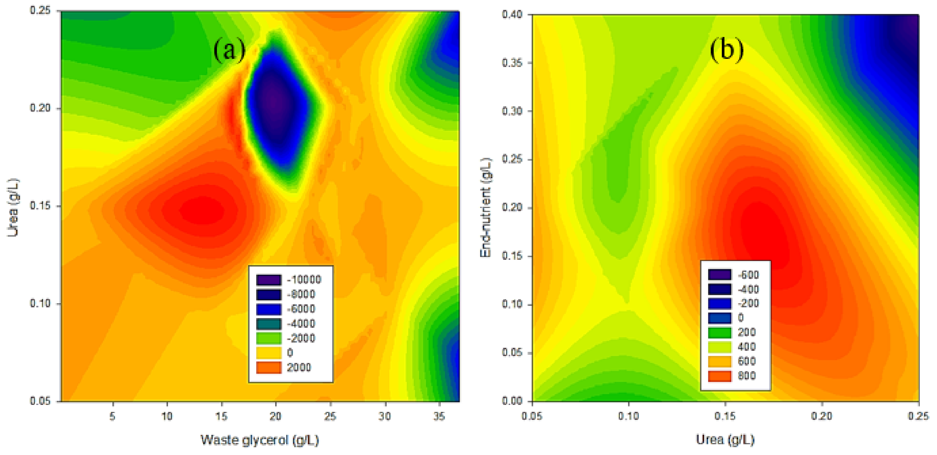
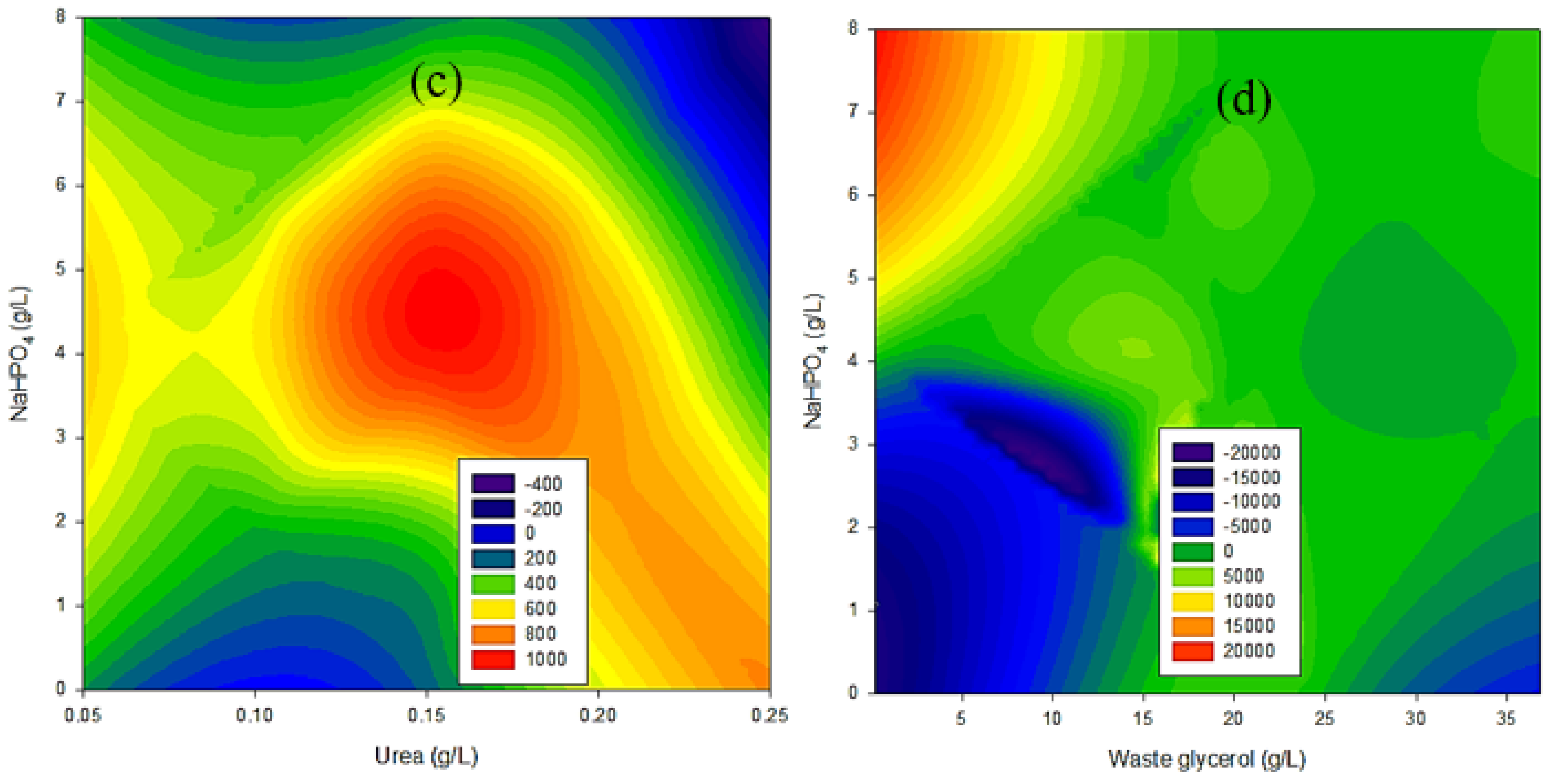
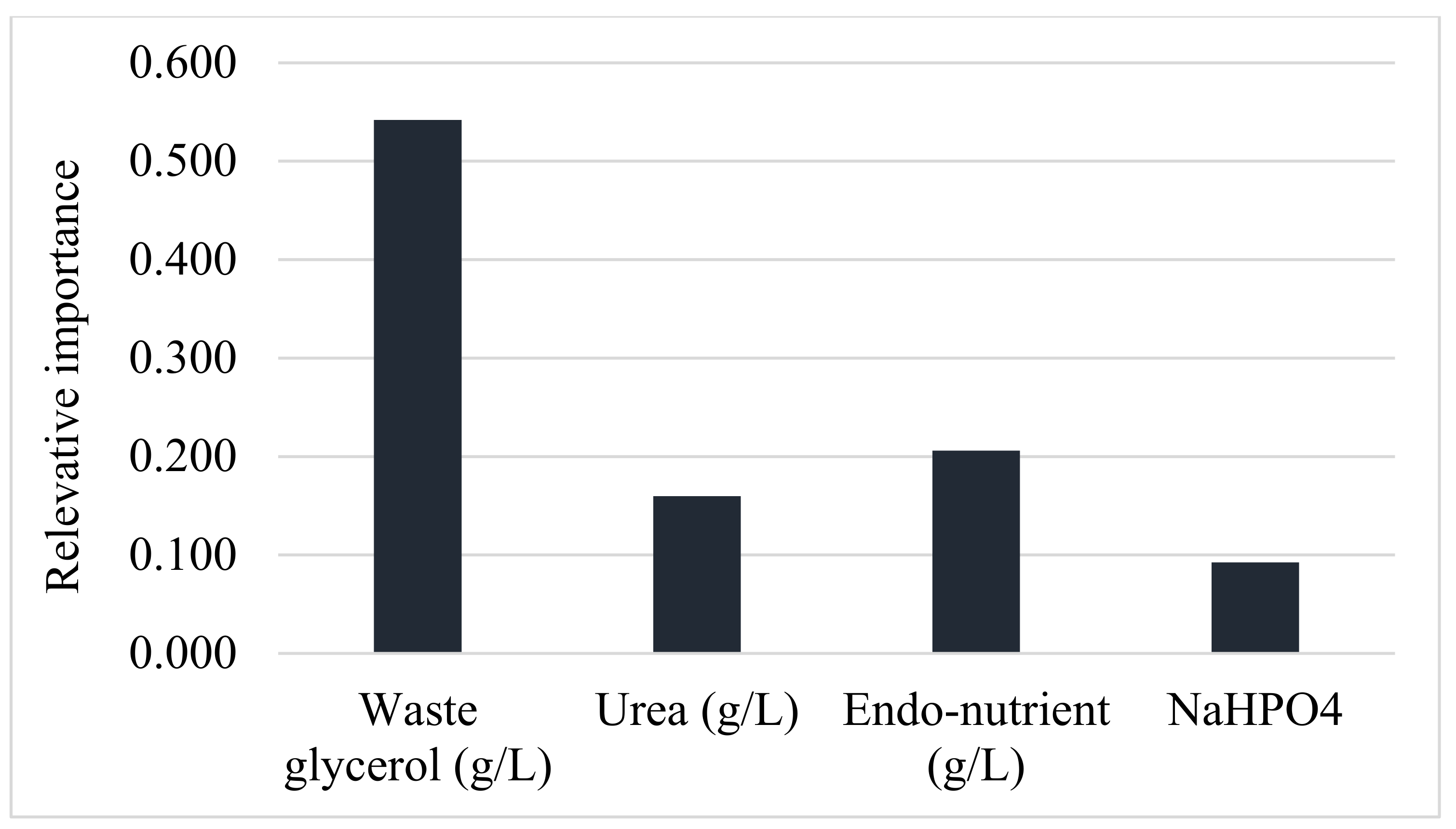
3.1. Parametric Analysis and Descriptive Statistics of the Data

The parametric analysis showing the relationship between input variables and hydrogen production is depicted by the contour plots in Figure 3. The contour plot analysis helped to determine what range of values of the input variables significantly influence the biohydrogen production based on the available experimental data. It was successfully employed in the analysis of fluid catalytic cracking catalysts, as reported by Ebrahimi and Ghazvini [28]. Figure 3a shows the effect of an interaction between waste glycerol and urea on biohydrogen production. The interaction effect of waste glycerol and urea on biohydrogen production can be seen to vary. Using a high concentration of urea inhibited biohydrogen production, as can be seen from the green color zone in Figure 3a, which is consistent with the report by Tratzi et al. 2022 [29]. However, at a concentration of urea in the range of 0.25–0.75 g/L and a waste glycerol concentration in the range of 5–20 g/L, a high volume of biohydrogen was produced. Also, in Figure 3b, high biohydrogen production was favored at a urea concentration range of 1.25–0.25 g/L using endo-nutrients up to 0.35 g/L. Figure 3c revealed that using Na2HPO4 in the range of 3–6 g/L while maintaining the concentration of urea between 0.1–0.175 can facilitate high biohydrogen production from waste glycerol. Figure 3d shows that the interaction between waste glycerol and Na2HPO4 has the most significant effects on biohydrogen production. It can be seen that high hydrogen production (up to 20,000 mL H2/L) was facilitated using waste glycerol in the range of 5–10 g/L and Na2HPO4 in the range of 6–8 g/L.
The descriptive statistical analysis of the dataset used for training the model is summarized in Table 2. The analysis revealed that waste glycerol is in the range of 0.23–36.81 g/L, with a mean value estimated at 21.39 g/L. The standard deviation and variance of waste glycerol datasets were calculated as 7.43 g/L and 55.27 g/L, respectively. The amount of urea used for the experiment varied in the range of 0.05 to 0.25 g/L, with a mean value of 0.15 g/L. The standard deviation and the variance were obtained as 0.05 g/L and 0 g/L, respectively. The Endo-nutrient amounts used for the experiment also varied from 0 to 0.4 mL/L, with the mean value calculated as 0.15. A standard deviation of 0.1 was obtained for the datasets. For Na2HPO4, the amount varied from 0 to 8 g/L with a mean of 3.93 g/L. The standard deviation and variance were estimated at 1.89 g/L and 3.57 g/L, respectively. The biohydrogen production was in the range of 117.46 to 1606.65 g/L, with the mean calculated as 582.98 g/L. The standard deviation and variance were calculated as 493.17 g/L and 243213.28 g/L, respectively.

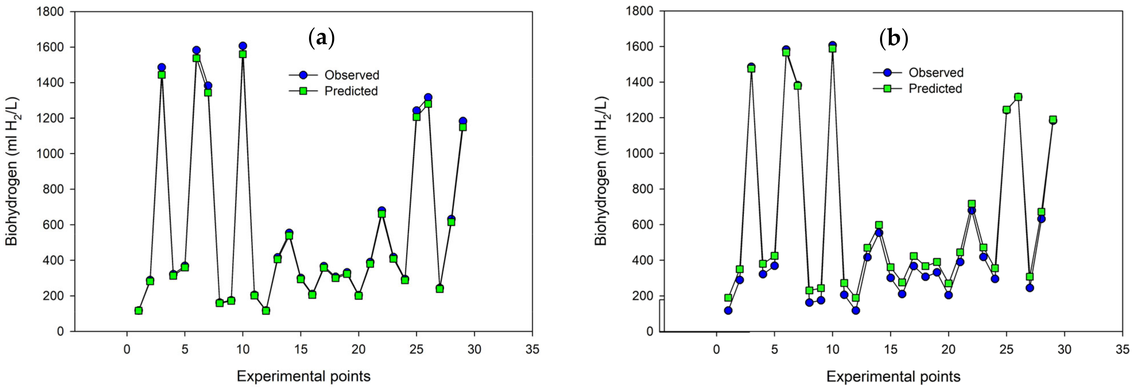
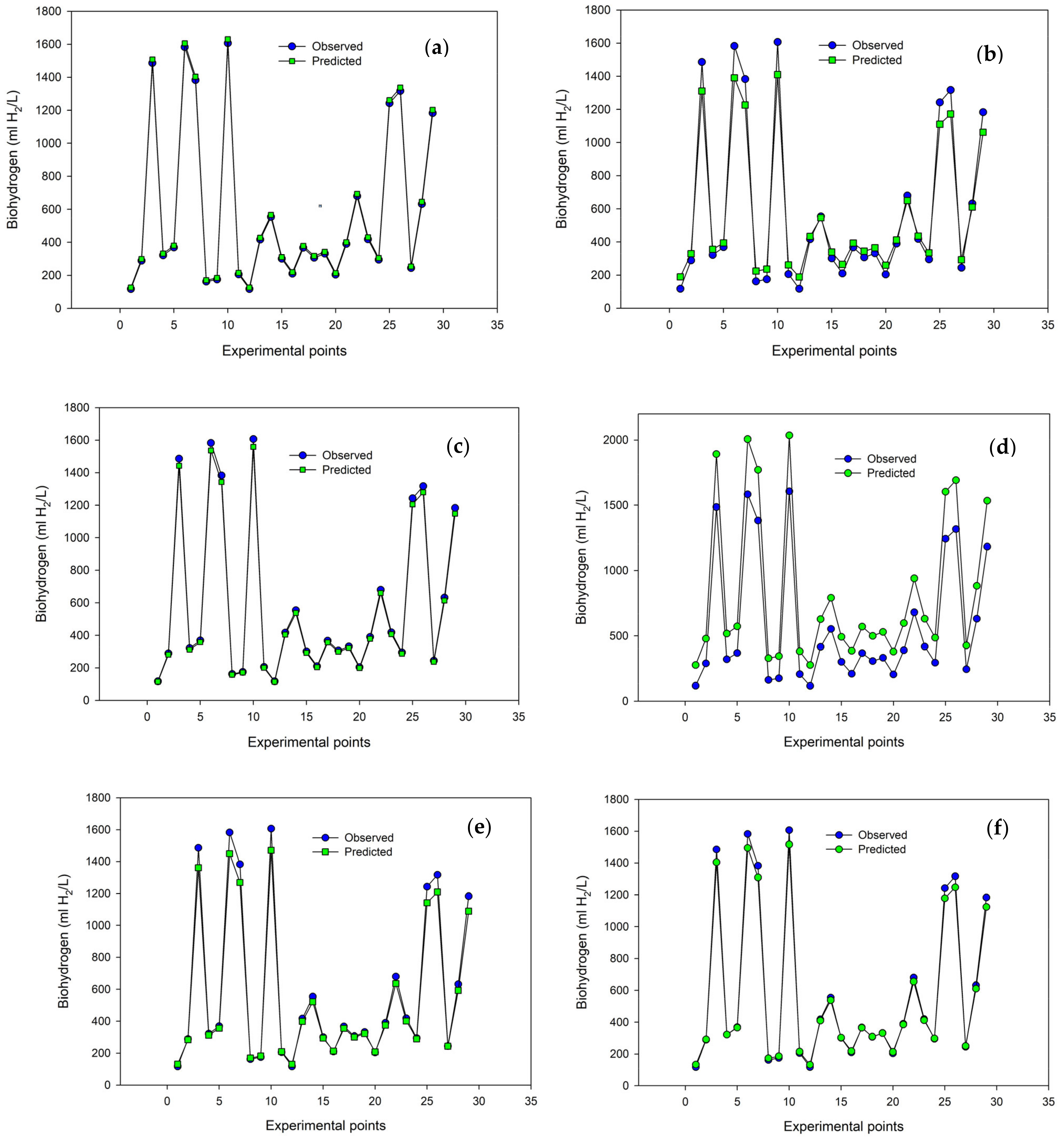
3.2. Model Performance

The performance of the RBFNN and MLPNN as a function of the RMSE, SEE, and R2 is summarized in Table 3. The RBFNN displayed great potential in predicting the biohydrogen production from waste glycerol. As shown in Figure 4a, the actual values depicted as “1” are consistent with the predicted values by RBFNN-1 depicted as “2”. On the contrary, poorer performance in the prediction of the biohydrogen from waste glycerol using the RBFNN-2 is observed in Figure 4b. Moreover, the superior performance of the RBFNN-1 model over the RBFNN-2 model can be further ascertained from the R2 and RMSE values of 0.903 and 53.31, respectively, obtained for the RBFNN-1 model. This implied that RBFNN-1 had a robust prediction with fewer errors compared to RBFNN-2, which had R2 and RMSE values of 0.419 and 301.55, respectively. A better performance of RBFNN-1 compared with RBFNN-2 could be attributed to the use of a standardized identity activation function compared to the non-standardized activation function used in RBFNN-2. The use of a standardized identity activation function has been reported to improve the performance of RBFNN [30]. The use of standardized identity as an activation function in the outer layer helps to prevent diminishing gradient problems and improve the computation performance of the RBFNN-1 model [31].
The performance of the MLPNNs with various configurations based on the hidden and outer layer activation functions optimized using a scaled conjugate gradient algorithm is depicted in Figure 5. It can be seen that all the MLPNN configurations optimized using the scaled conjugate gradient algorithms were robust in their predictive modeling of the interconnectivity between the input variables and the targeted output (biohydrogen production), with the exception of MLPNN-2. The actual volume of biohydrogen produced per liter of waste glycerol in Figure 5a,c–e was consistent with the values predicted by the MLPNN-1, MLPNN-3, MLPNN-4, and MLPNN-5, respectively. This implied that the combination of a hyperbolic tangent as the activation function for the hidden layer and identity as the activation function for the outer layer resulted in a robust performance in predicting biohydrogen production. This can be further ascertained from a high R2 value of 0.920 and a low RMSE value of 21.48. Minimal errors were obtained from training and testing the MLPNN-1 with the experimental data. However, improved performance in the predictability of the model was obtained using MLPNN-3, MLPNN-4, and MLPNN-5, as indicated by the R2 values of 0.969, 0.954, and 0.939, respectively, and low RMSE values. This implied that the nature of the activation function used in the hidden and outer layers significantly influenced the model’s performance [32]. Using the scaled conjugate gradient optimization algorithm, the MLPNN-3 with hyperbolic tangent as the hidden layer activation function and sigmoid as the outer layer activation function had the best predictive performance, as indicated by an R2 of 0.969. It is obvious that using hyperbolic tangent as an activation function at the hidden and outer layers did not result in good predictability by the model, as indicated by an R2 of 0.433.
The performance of the MLPNN models with various configurations optimized using gradient descent algorithms is depicted in Figure 6. It can be seen that all the model configurations displayed robust performance in modeling the prediction of biohydrogen production from waste glycerol. Compared to MLPNN optimization using the scaled conjugate gradient algorithm, better performances were obtained for MLPNN by using the gradient descent optimization algorithm. The gradient descent optimization algorithm had the advantage of robust computational efficiency, whereby a stable error gradient was produced, resulting in stable convergence [33,34]. Moreover, it can be seen that the use of various configurations of activation functions in the hidden and outer layers of the MLPNN optimized using the gradient descent algorithm significantly influenced the model’s predictability. Although all the models displayed robust performance based on their high R2 value, which was greater than 0.940, MLPNN-7 with hyperbolic tangent as the hidden layer activation function and Sigmoid as the outer layer activation function displayed the best performance, as indicated by an R2 of 0.978 and a RMSE of 9.91. This performance was consistent with the best configuration using the scaled gradient descent optimization algorithm. For all the models, the actual values of the volume of biohydrogen produced per liter of waste glycerol were in close proximity with the predicted values, as shown in Figure 6a–e. The training and testing of the experimental data in the models resulted in low errors, as indicated by the low SSE values.
The level of importance of the analysis of how the input variables influence the predicted values is depicted in Figure 7. It can be seen that all the input variables, namely waste glycerol, Urea, Endo-nutrient, and Na2PO4, had varying levels of influence on the predicted biohydrogen production. However, waste glycerol with the highest level of importance value of 0.542 had the most significant influence on the predicted biohydrogen production.

3.3. Comparison of the Best Model with Literature and Implications of the Study

The performance analysis of the various models used in this study, as summarized in Table 2, revealed that MLPNN configured using the hyperbolic tangent in the hidden layer and sigmoid at the outer layer with a gradient descent optimization algorithm producing the best prediction of biohydrogen from the biodiesel waste. This is evidenced by the highest R2 value of 0.978 and the lowest RMSE value of 9.91 mL H2/L of biodiesel waste. The robust performance of the model in modeling the prediction of biohydrogen production could be attributed to the unique characteristics of the hyperbolic tangent as well as the activation at the hidden layer [35]. The hyperbolic activation function enables rapid network convergence at the hidden layer, thereby complementing the sigmoid activation function and facilitating a robust prediction [36]. The sigma activation function’s primary goal is to keep the predicted or output value inside a certain bound, which contributes to the model’s effectiveness and precision [37]. Besides, it is generally accepted that the best method for optimizing neural networks and other machine-learning algorithms is using gradient descent. Gradient descent as an iterative optimization algorithm has the advantage of reducing the cost function to obtain a model that can accurately predict a targetted output [38]. The difference between the model’s anticipated output and the actual output was measured by the cost function (C) or the loss function.
The performance of the best model in this study is comparable with similar MLP-neural network configurations that have been successfully employed to model geothermal power generation [39], hydrogen solubility in hydrocarbon fuels [40], prediction of corrosion inhibition performances of ionic liquids [41], the interfacial tension of the hydrogen-brine system [42], and lignin extraction from oil palm biomass [43] (Table 4). Various models have displayed robust performance in modeling the target model output, as indicated by high R2 and low RMSE values. The slight variation in the performance indicator of the best model in this study and those reported in the literature can be attributed to the peculiarity of the datasets, the differences in training algorithms, and the nature of activation functions.
Since the MLPNN can recognize all conceivable interactions between predictor variables, numerous training methods, and the capacity to implicitly detect complicated nonlinear connections between dependent and independent variables, model algorithms can be employed to determine the most important parameters that influence biohydrogen production from biodiesel waste such as glycerol, considering all possible input parameters. Besides, using the existing data to model the prediction of biohydrogen could help optimize the process, thereby preventing material loss, enhancing process safety, and eventually saving costs. However, the study is limited since all the available hyperparameters in the model configurations have not been fully exhausted. Hence, future research could consider the effect of various layers and perhaps varying the number of artificial neurons in the hidden layer as well as employing the possibility of more training algorithms.

4. Conclusions

In this study, a modeling approach was employed to understand the role of process variables in biohydrogen production from biodiesel production waste. Twelve models, mainly MLPNN and RBFNN, were configured by varying the activation functions in the hidden and outer layers under two different types of optimization algorithms. Both the MLPNN and RBFNN performances were significantly influenced by the type of activation function used in the hidden and outer layers. The use of softmax and identity activation functions in the hidden and outer layers of the RBFNN model did not show impressive performance. Whereas an improved performance was observed using exponential and standardized identities at the hidden and outer layers of the RBFNN model, respectively. The MLPNN models displayed superior predictive performance compared to the RBFNN model. The MLPNN model with hyperbolic tangent and sigmoid activation functions at the hidden and outer layers incorporated with the gradient descent optimization algorithm displayed the best performance, which was reflected in the high R2 value of 0.978.

Author Contributions

Conceptualization, S.S.H. and B.V.A.; methodology, S.S.H. and B.V.A.; software, S.S.H.; validation, S.S.H., B.V.A. and Z.A.A.; formal analysis, B.V.A.; investigation, B.V.A.; resources, S.S.H.; data curation, Z.A.A. and M.M.A.A.; writing—original draft preparation, B.V.A.; writing—review and editing, S.S.H. and M.M.A.A.; visualization, S.S.H.; supervision, S.S.H.; project administration, S.S.H.; funding acquisition, S.S.H. All authors have read and agreed to the published version of the manuscript.

Funding

This research was supported by the Deanship of Scientific Research and the Vice Presidency for Graduate Studies and Scientific Research at King Faisal University, Saudi Arabia [Old Project No. Grant 571 and New project No. Grant 1884].

Data Availability Statement

Not applicable.

Conflicts of Interest

The authors declare no conflict of interest.

References

  1. Gabrielli, P.; Gazzani, M.; Mazzotti, M. The Role of Carbon Capture and Utilization, Carbon Capture and Storage, and Biomass to Enable a Net-Zero-CO2 Emissions Chemical Industry. Ind. Eng. Chem. Res. 2020, 59, 7033–7045. [Google Scholar] [CrossRef] [Green Version]
  2. Lin, B.; Raza, M.Y. Analysis of energy related CO2 emissions in Pakistan. J. Clean. Prod. 2019, 219, 981–993. [Google Scholar] [CrossRef]
  3. Shahsavari, A.; Akbari, M. Potential of solar energy in developing countries for reducing energy-related emissions. Renew. Sustain. Energy Rev. 2018, 90, 275–291. [Google Scholar] [CrossRef]
  4. Zhou, N.; Price, L.; Yande, D.; Creyts, J.; Khanna, N.; Fridley, D.; Lu, H.; Feng, W.; Liu, X.; Hasanbeigi, A.; et al. A roadmap for China to peak carbon dioxide emissions and achieve a 20% share of non-fossil fuels in primary energy by 2030. Appl. Energy 2019, 239, 793–819. [Google Scholar] [CrossRef]
  5. Hu, Y.; Ren, S.; Wang, Y.; Chen, X. Can carbon emission trading scheme achieve energy conservation and emission reduction? Evidence from the industrial sector in China. Energy Econ. 2020, 85, 104590. [Google Scholar] [CrossRef]
  6. Williams, J.H.; Jones, R.A.; Haley, B.; Kwok, G.; Hargreaves, J.; Farbes, J.; Torn, M.S. Carbon-Neutral Pathways for the United States. AGU Adv. 2021, 2, e2020AV000284. [Google Scholar] [CrossRef]
  7. Sinsel, S.R.; Riemke, R.L.; Hoffmann, V.H. Challenges and solution technologies for the integration of variable renewable energy sources—A review. Renew. Energy 2020, 145, 2271–2285. [Google Scholar] [CrossRef]
  8. Qazi, A.; Hussain, F.; Rahim, N.A.B.D.; Hardaker, G.; Alghazzawi, D.; Shaban, K.; Haruna, K. Towards Sustainable Energy: A Systematic Review of Renewable Energy Sources, Technologies, and Public Opinions. IEEE Access 2019, 7, 63837–63851. [Google Scholar] [CrossRef]
  9. Queneau, Y.; Han, B. Biomass: Renewable carbon resource for chemical and energy industry. Innovations 2022, 3, 100184. [Google Scholar] [CrossRef]
  10. Alatzas, S.; Moustakas, K.; Malamis, D.; Vakalis, S. Biomass Potential from Agricultural Waste for Energetic Utilization in Greece. Energies 2019, 12, 1095. [Google Scholar] [CrossRef]
  11. Ahorsu, R.; Medina, F.; Constantí, M. Significance and Challenges of Biomass as a Suitable Feedstock for Bioenergy and Biochemical Production: A Review. Energies 2018, 11, 3366. [Google Scholar] [CrossRef] [Green Version]
  12. Osman, A.I.; Mehta, N.; Elgarahy, A.M.; Al-Hinai, A.; Al-Muhtaseb, A.H.; Rooney, D.W. Conversion of biomass to biofuels and life cycle assessment: A review. Environ. Chem. Lett. 2021, 19, 4075–4118. [Google Scholar] [CrossRef]
  13. Tabassum, N.; Pothu, R.; Pattnaik, A.; Boddula, R.; Balla, P.; Gundeboyina, R.; Challa, P.; Rajesh, R.; Perugopu, V.; Mameda, N.; et al. Heterogeneous Catalysts for Conversion of Biodiesel-Waste Glycerol into High-Added-Value Chemicals. Catalysts 2022, 12, 767. [Google Scholar] [CrossRef]
  14. Schwengber, C.A.; Alves, H.J.; Schaffner, R.A.; Da Silva, F.A.; Sequinel, R.; Bach, V.R.; Ferracin, R.J. Overview of glycerol reforming for hydrogen production. Renew. Sustain. Energy Rev. 2016, 58, 259–266. [Google Scholar] [CrossRef]
  15. Sittijunda, S.; Reungsang, A. Media optimization for biohydrogen production from waste glycerol by anaerobic thermophilic mixed cultures. Int. J. Hydrogen Energy 2012, 37, 15473–15482. [Google Scholar] [CrossRef]
  16. Hossain, S.S.; Ayodele, B.V.; Almithn, A. Predictive Modeling of Bioenergy Production from Fountain Grass Using Gaussian Process Regression: Effect of Kernel Functions. Energies 2022, 15, 5570. [Google Scholar] [CrossRef]
  17. Hossain, S.K.S.; Ali, S.S.; Rushd, S.; Ayodele, B.V.; Cheng, C.K. Interaction effect of process parameters and Pd-electrocatalyst in formic acid electro-oxidation for fuel cell applications: Implementing supervised machine learning algorithms. Int. J. Energy Res. 2022. [Google Scholar] [CrossRef]
  18. Cinar, A.C. Training Feed-Forward Multi-Layer Perceptron Artificial Neural Networks with a Tree-Seed Algorithm. Arab. J. Sci. Eng. 2020, 45, 10915–10938. [Google Scholar] [CrossRef]
  19. Gülcü, Ş. An Improved Animal Migration Optimization Algorithm to Train the Feed-Forward Artificial Neural Networks. Arab. J. Sci. Eng. 2022, 47, 9557–9581. [Google Scholar] [CrossRef]
  20. Alsaffar, M.A.; Ayodele, B.V.; Mustapa, S.I. Scavenging carbon deposition on alumina supported cobalt catalyst during renewable hydrogen-rich syngas production by methane dry reforming using artificial intelligence modeling technique. J. Clean. Prod. 2020, 247, 119168. [Google Scholar] [CrossRef]
  21. Nabavi-Pelesaraei, A.; Bayat, R.; Hosseinzadeh-Bandbafha, H.; Afrasyabi, H.; Chau, K.W. Modeling of energy consumption and environmental life cycle assessment for incineration and landfill systems of municipal solid waste management—A case study in Tehran Metropolis of Iran. J. Clean. Prod. 2017, 148, 427–440. [Google Scholar] [CrossRef]
  22. Yogeswari, M.K.; Dharmalingam, K.; Mullai, P. Implementation of artificial neural network model for continuous hydrogen production using confectionery wastewater. J. Environ. Manag. 2019, 252, 109684. [Google Scholar] [CrossRef]
  23. Hossain, M.A.; Ayodele, B.V.; Cheng, C.K.; Khan, M.R. Artificial neural network modeling of hydrogen-rich syngas production from methane dry reforming over novel Ni/CaFe2O4 catalysts. Int. J. Hydrogen Energy 2016, 41, 11119–11130. [Google Scholar] [CrossRef] [Green Version]
  24. Zhao, Z.; Lou, Y.; Chen, Y.; Lin, H.; Li, R.; Yu, G. Prediction of interfacial interactions related with membrane fouling in a membrane bioreactor based on radial basis function artificial neural network (ANN). Bioresour. Technol. 2019, 282, 262–268. [Google Scholar] [CrossRef] [PubMed]
  25. Aghbashlo, M.; Hosseinpour, S.; Tabatabaei, M.; Dadak, A.; Younesi, H.; Najafpour, G. Multi-objective exergetic optimization of continuous photo-biohydrogen production process using a novel hybrid fuzzy clustering-ranking approach coupled with Radial Basis Function (RBF) neural network. Int. J. Hydrogen Energy 2016, 41, 18418–18430. [Google Scholar] [CrossRef]
  26. Faris, H.; Aljarah, I.; Mirjalili, S. Improved monarch butterfly optimization for unconstrained global search and neural network training. Appl. Intell. 2018, 48, 445–464. [Google Scholar] [CrossRef]
  27. Garson, G.D. Comparison of Neural Network Analysis of Social Science Data. Soc. Sci. Comput. Rev. 1991, 9, 399–434. [Google Scholar] [CrossRef]
  28. Afshar Ebrahimi, A.; Foroutan Ghazvini, S. Experimental attrition study of FCC catalysts through 2D/3D contour plots and response surface models. Powder Technol. 2018, 336, 80–84. [Google Scholar] [CrossRef]
  29. Tratzi, P.; Ta, D.T.; Zhang, Z.; Torre, M.; Battistelli, F.; Manzo, E.; Paolini, V.; Zhang, Q.; Chu, C.; Petracchini, F. Sustainable additives for the regulation of NH3 concentration and emissions during the production of biomethane and biohydrogen: A review. Bioresour. Technol. 2022, 346, 126596. [Google Scholar] [CrossRef]
  30. Carreras, J.; Kikuti, Y.Y.; Miyaoka, M.; Hiraiwa, S.; Tomita, S.; Ikoma, H.; Kondo, Y.; Ito, A.; Nakamura, N.; Hamoudi, R. A Combination of Multilayer Perceptron, Radial Basis Function Artificial Neural Networks and Machine Learning Image Segmentation for the Dimension Reduction and the Prognosis Assessment of Diffuse Large B-Cell Lymphoma. AI 2021, 2, 106–134. [Google Scholar] [CrossRef]
  31. Lv, Z.; Xiao, F.; Wu, Z.; Liu, Z.; Wang, Y. Hand gestures recognition from surface electromyogram signal based on self-organizing mapping and radial basis function network. Biomed. Signal Process. Control 2021, 68, 102629. [Google Scholar] [CrossRef]
  32. Moosavi, S.R.; Wood, D.A.; Ahmadi, M.A.; Choubineh, A. ANN-Based Prediction of Laboratory-Scale Performance of CO2-Foam Flooding for Improving Oil Recovery. Nat. Resour. Res. 2019, 28, 1619–1637. [Google Scholar] [CrossRef]
  33. Dogo, E.M.; Afolabi, O.J.; Nwulu, N.I.; Twala, B.; Aigbavboa, C.O. A Comparative Analysis of Gradient Descent-Based Optimization Algorithms on Convolutional Neural Networks. In Proceedings of the International Conference on Computational Techniques, Electronics and Mechanical Systems (CTEMS 2018), Belagavi, India, 21–23 December 2018. [Google Scholar]
  34. Mele, M.; Magazzino, C.; Schneider, N.; Nicolai, F. Revisiting the dynamic interactions between economic growth and environmental pollution in Italy: Evidence from a gradient descent algorithm. Environ. Sci. Pollut. Res. 2021, 28, 52188–52201. [Google Scholar] [CrossRef]
  35. Kaloev, M.; Krastev, G. Comparative analysis of activation functions used in the hidden layers of deep neural networks. In Proceedings of the 2021 3rd International Congress on Human-Computer Interaction, Optimization and Robotic Applications (HORA), Ankara, Turkey, 11–13 June 2021; pp. 1–5. [Google Scholar] [CrossRef]
  36. Rasamoelina, A.D.; Adjailia, F.; Sinčák, P. A review of activation function for artificial neural network. In Proceedings of the 2020 IEEE 18th World Symposium on Applied Machine Intelligence and Informatics (SAMI), Herl’any, Slovakia, 23–25 January 2020; pp. 281–286. [Google Scholar] [CrossRef]
  37. Wang, Y.; Li, Y.; Song, Y.; Rong, X. The influence of the activation function in a convolution neural network model of facial expression recognition. Appl. Sci. 2020, 10, 1897. [Google Scholar] [CrossRef] [Green Version]
  38. Hu, Q.; Cai, Y.; Shi, Q.; Xu, K.; Yu, G.; Ding, Z. Iterative algorithm induced deep-unfolding neural networks: Precoding design for multiuser MIMO systems. IEEE Trans. Wirel. Commun. 2020, 20, 1394–1410. [Google Scholar] [CrossRef]
  39. Khosravi, A.; Syri, S. Modeling of geothermal power system equipped with absorption refrigeration and solar energy using multilayer perceptron neural network optimized with imperialist competitive algorithm. J. Clean. Prod. 2020, 276, 124216. [Google Scholar] [CrossRef]
  40. Mohammadi, M.R.; Hadavimoghaddam, F.; Atashrouz, S.; Hemmati-Sarapardeh, A.; Abedi, A.; Mohaddespour, A. Application of robust machine learning methods to modeling hydrogen solubility in hydrocarbon fuels. Int. J. Hydrogen Energy 2022, 47, 320–338. [Google Scholar] [CrossRef]
  41. Quadri, T.W.; Olasunkanmi, L.O.; Fayemi, O.E.; Akpan, E.D.; Lee, H.S.; Lgaz, H.; Verma, C.; Guo, L.; Kaya, S.; Ebenso, E.E. Multilayer perceptron neural network-based QSAR models for the assessment and prediction of corrosion inhibition performances of ionic liquids. Comput. Mater. Sci. 2022, 214, 111753. [Google Scholar] [CrossRef]
  42. Ng, C.S.W.; Djema, H.; Amar, M.N.; Ghahfarokhi, A.J. Modeling interfacial tension of the hydrogen-brine system using robust machine learning techniques: Implication for underground hydrogen storage. Int. J. Hydrogen Energy 2022, 47, 39595–39605. [Google Scholar] [CrossRef]
  43. Rashid, T.; Taqvi SA, A.; Sher, F.; Rubab, S.; Thanabalan, M.; Bilal, M.; ul Islam, B. Enhanced lignin extraction and optimisation from oil palm biomass using neural network modelling. Fuel 2021, 293, 120485. [Google Scholar] [CrossRef]
Figure 1. Overall process flow for the modeling of biohydrogen production from waste glycerol.
Applsci 12 12914 g001
Figure 2. The architecture of a multilayer perceptron and radial basis function neural networks.
Applsci 12 12914 g002
Figure 3. Contour plots showing the interaction between (a) urea and waste glycerol (b) Endo-nutrient and urea (c) Na2HPO4 and urea (d) Na2HPO4 and waste glycerol.
Applsci 12 12914 g003aApplsci 12 12914 g003b
Figure 4. Comparison between the actual and predicted biohydrogen using (a) RBFNN-1 (b) RBFNN-2.
Applsci 12 12914 g004
Figure 5. Comparison between the actual and predicted biohydrogen using (a) MLPNN-1 (b) MLPNN-2 (c) MLPNN-3 (d) MLPNN-4 (e) MLPNN-5 (f) MLPNN-6 with a scaled conjugate gradient optimization algorithm.
Applsci 12 12914 g005
Figure 6. Comparison between actual and predicted biohydrogen using (a) MLPNN-7 (b) MLPNN-8 (c) MLPNN-9 (d) MLPNN-10 (e) MLPNN-11 (f) MLPNN-12 with a gradient descent optimization algorithm.
Applsci 12 12914 g006
Figure 7. Analysis of the relative importance of input variables on predicted biohydrogen production.
Applsci 12 12914 g007
Table 1. Summary of the various MLPNN and RBFNN configurations used.
ModelThe Activation Function in the Hidden LayerThe Activation Function in the Outer LayerOptimization Algorithm for TrainingNumber of Units in the Hidden Layers
MLPNN 1Hyperbolic tangentIdentityScaled conjugate gradient10
MLPNN 2Hyperbolic tangentHyperbolic tangentScaled conjugate gradient10
MLPNN 3Hyperbolic tangentSigmoidScaled conjugate gradient10
MLPNN 4SigmoidIdentityScaled conjugate gradient10
MLPNN 5SigmoidHyperbolic tangentScaled conjugate gradient10
MLPNN 6SigmoidSigmoidScaled conjugate gradient10
MLPNN 7Hyperbolic tangentIdentitygradient descent10
MLPNN 8Hyperbolic tangentSigmoidgradient descent10
MLPNN 9Hyperbolic tangentHyperbolic tangentgradient descent10
MLPNN 10SigmoidIdentitygradient descent10
MLPNN 11SigmoidHyperbolic tangentgradient descent10
MLPNN 12SigmoidSigmoidgradient descent10
RBFNN-1SoftmaxIdentityordinary10
RBFNN-2SoftmaxStandardized identitystandard10
Table 2. Descriptive statistics for input and targeted variables.
ParametersRangeMinimumMaximumMeanStandard DeviationVariance
Waste glycerol (g/L)36.580.2336.8121.397.4355.27
Urea (g/L)0.200.050.250.150.050.00
Endo-nutrient (mL/L)0.400.000.400.190.100.01
Na2HPO4 (g/L)8.000.008.003.931.893.57
HP (mL H2/L)1489.19117.461606.65582.98493.17243,213.28
Table 3. Summary of performance analysis for the models.
ModelRMSESSE-TrainingSSE-TestingR2
RBFNN-153.311.2530.0240.903
RBFNN-2212.253.0820.0170.736
MLPNN-121.481.0830.0210.920
MLPNN-251.994.0520.0000.433
MLPNN-312.660.0340.0100.969
MLPNN-488.140.5670.0740.954
MLPNN-559.260.3580.0380.939
MLPNN-629.630.0280.0180.957
MLPNN-7258.120.2500.2070.965
MLPNN-89.910.0270.0030.978
MLPNN-938.430.3170.0760.934
MLPNN-1043.720.4930.1980.948
MLPNN-1116.200.1110.0060.977
MLPNN-1215.090.0350.0190.959
Table 4. Comparison of the best model with the literature.
Model-TypeObjectiveRMSER2Reference
MLPNN (Hyperbolic tangent as the hidden layer activation function and sigmoid as the outer layer activation function To model the prediction of biohydrogen production from biodiesel production waste9.910.978This study
MLP coupled with imperialist competitive algorithmTo model geothermal power generation2.240.997Khosravi and Syri [39]
MLP coupled with levenberg marquardt training algorithmTo model hydrogen solubility in hydrocarbon fuels0.020.993Mohammadi et al. [40]
MLPNNTo model the prediction of corrosion inhibition performances of ionic liquids5.470.970Quadri et al. [41]
MLP- coupled with levenberg marquardt training algorithmTo model the interfacial tension of hydrogen-brine system0.180.999Ng et al. [42]
MLP coupled with levenberg marquardt training algorithm and Sigmoid function as activation functionTo model lignin extraction from oil palm biomass1.130.993Rashid et al. [43]
Publisher’s Note: MDPI stays neutral with regard to jurisdictional claims in published maps and institutional affiliations.

