
Optimization of Driving Speed of Electric Train Using Dynamic Programming Based on Multi-Weighted Cost Function


Korea Railroad Research Institute, 176 Cheoldobangmulgwan-ro, Uiwang 16105, Gyeonggi-do, Republic of Korea
*
Author to whom correspondence should be addressed.
Appl. Sci. 2022, 12(24), 12857; https://doi.org/10.3390/app122412857
Submission received: 7 November 2022
/
Revised: 7 December 2022
/
Accepted: 12 December 2022
/
Published: 14 December 2022
(This article belongs to the Topic Energy Saving and Energy Efficiency Technologies)
Abstract
:Trains are a large-capacity means of transportation, and they are preferred for long as well as short distances. Although trains are one of the most efficient modes of transportation for freight and passengers, they consume a significant amount of energy. Therefore, energy-efficient approaches have been studied over the years. Various optimal-control methods that integrate dynamic programming (DP) algorithms have been introduced to reduce the overall energy consumption. The purpose of optimizing the operation speed of the train according to the operating conditions using the DP algorithm is to find a speed profile that consumes minimum energy, under the condition that the target travel time is satisfied according to the given mileage. Here, a specific weight is applied to the cost function to find a velocity profile that satisfies the target travel time. In this case, the computation time increases proportionally to the number of times the weight is changed. In addition, because the weight versus the target travel time has a non-linear characteristic, various approaches have been proposed to reduce the number of iterations according to the weight change to satisfy the target travel time. This study suggests a method to quickly and effectively find the optimal solution for electric trains in a different way from previous studies. We present a DP algorithm for matrix processing, by arranging multiple weights within the applicable minimum and maximum weights and applying them to the cost function. The time taken to find the optimal solution can be reduced by half compared to the existing one, and the travel time and energy consumption corresponding to each weight can be checked at once. In addition, this result can be used as an indicator for effectively changing or establishing an electric-train operation plan. For a detailed comparison between the proposed and existing methods, the execution time results for each number of weights under the same calculation conditions are presented. In addition, to verify that there are no errors in the multi-weighting process, some of the multi-weighting coefficients were used to check whether the speed profile in the single-weighted calculation method was consistent.
1. Introduction
As the scale of global industrial activities increases, energy consumption continues to increase. Accordingly, demands for the efficient use of the Earth’s limited resources as well as environmental protection of the Earth are increasing. Energy consumption is continuously increasing not only in industrial processes but also in large buildings and transportation systems, requiring their efficient operation. The electric railway system is one of the fields that demand excessive energy. Several studies have attempted to improve the energy efficiency of railways. More than 80% of the total operating-energy consumption of railways is utilized by the train system, while more than 60% of the energy is consumed by the trains’ power systems [1]. Therefore, this study focuses on improving the driving energy efficiency of electric trains specifically; whenever a train is mentioned, this means an electric train.
Several methods for optimizing train-running energy have been presented in recent years. In an early train-operation optimization study, Milroy discussed, in 1980, how to operate trains under minimum-energy control according to timetables and operational constraints [2]. Few studies have applied the evolutionary algorithm (EA) [3,4,5]; in 2011, Chevrier et al. searched various solutions in a continuous search space based on an evolutionary algorithm to address a multipurpose problem involving three criteria: reduced travel time, reduced delay, and minimized energy consumption [3]. In 2015, Huang et al. proposed an energy-efficient approach to reduce traction energy, by optimizing train operation for multiple interstations using a multi-population genetic algorithm (MPGA) [4]. In 2020, Fernández-Rodríguez presented a simulation-based optimization algorithm to solve the eco-driving problem subject with multiple target-time constraints, by applying the differential evolution algorithm [5]. In 2013, Lu et al. proposed a distance-based train-trajectory search model that applies three optimization algorithms (ants colony optimization (ACO), dynamic programming (DP), and genetic algorithm (GA)) to find the optimal train speed trajectory [6]. In 2016, Huang et al. proposed a fast and effective optimization algorithm based on a two-step method for finding an optimal curve using a maximum–minimum colony optimization system with an approximation of a discrete combinatorial optimization model [7]. In 2011, Kim et al. proposed an optimization method that minimizes energy consumption by considering track alignment, speed limit, and schedule compliance based on the simulated annealing (SA) algorithm [8]. In 2013, Xie et al. developed a simulation annealing algorithm to find the optimal coasting point and proposed an optimization method that minimizes energy consumption by comprehensively considering the speed limit, track alignment, and travel time [9].
A recent study [10] compared the pros and cons of the three primarily used methods for optimizing driving energy—DP, gradient method (GM), and sequential quadratic programming (SQP). According to the analysis results of this study, DP is suitable for design considering speed limit and disturbances such as running resistance and gradient resistance, but it is not advantageous for optimizing calculation speed and multiple inputs. Here, operational constraints such as speed limits and disturbances are used for train models and DP based on train running position using running-track data tables. GM is not suitable for design considering disturbance or speed limit, but it has a fast calculation speed and is suitable for optimizing multiple inputs. In addition, SQP is slow in calculation speed and unfavorable considering disturbance or speed limit, but it has significant multi-input processing and practical applicability. In 2014, Ozatay et al. proposed a DP algorithm to generate a driving route by sending the driver’s destination information to a server in the cloud, collecting traffic and geographic information of the route, and using it to determine the optimal speed trajectory [11]. In 2004, Ko et al. applied DP to generate an optimal train running trajectory that minimizes the total energy consumption under a fixed starting point and destination, regulated running time, limited electric power, and electric braking in a train driven by a variable-voltage–variable-frequency controlled induction motor/generator [12]. In 2009, Miyatake et al. applied the DP algorithm to determine the optimal acceleration and deceleration in a wireless-mode railway vehicle [13]. In [14], a DP algorithm was used to address a problem that satisfies the constraints of time, distance, and speed in three dimensions. The authors in [15] used an approach wherein weights were applied to the cost function in the two-dimensional space of distance and speed to reduce the burden of calculation time due to multi-dimensionality. The driving mode for energy optimization was determined by classifying the electric-train operating conditions into four modes (acceleration, cruising, coasting, and braking) and optimizing the sequence of these modes.
In [15,16,17,18,19,20], to solve the problem of energy optimization in cases when the travel distance and the target travel time are fixed, a weight is applied to the cost function and is repeatedly changed until the target travel time is satisfied. To reduce the computational time, Monastyrsky first applied the weighting factor to reduce the three-dimensional DP to a two-dimensional DP [19]. In the first study [19] that optimized train operation by applying weights to DP, the topic of obtaining weight coefficients is not mentioned at all. In [15], a solution that satisfies the target condition was obtained after the weights were changed at least nine times. Here, numerical iterative approaches, such as the bisection method or secant method, are used to find the optimal weights. Based on the four basic operating modes (acceleration, cruising, coasting, and braking), Lukas et al. determined the energy-optimization trajectory by optimizing the sequence of the operating modes and their corresponding switching points [16]. Mensing et al. used an optimization method selected in consideration of the traffic constraints, unlike previous research results, for eco-driving in car operation [17]. Themann et al. described an optimization approach and presented a method for determining suitable optimization parameters to consider drivers’ preferences [18]. Among the three optimization algorithms (ACO, DP, and GA), DP yielded the best results in energy optimization, but more time was required in terms of calculation time [6]. In this study, the DP method was selected as an optimization method considering the adaptability to the disturbance and the speed limit within the operating route.
Due to the nature of train operation, if the distance between stations is fixed, it is operated according to the timetable, and, thus, strict adherence to the arrival time is essential. Therefore, in several existing studies, to find a speed profile that optimizes energy while satisfying given constraints, such as distance, arrival time, speed limit, gradient, and curve, a weight is applied to the cost function and is repeatedly changed to find a velocity profile that satisfies the target travel time. Here, the time-consuming process of finding the optimal solution that reflects this change is repeated whenever the weights are changed.
This paper presents a method to shorten the iterative process of changing the weights and finding the optimal solution for electric trains. To this end, we, herein, propose an approach to obtain an optimal solution, by composing weights in an array multiplexed by a desired interval and number and processing them in batches using the DP algorithm. In this algorithm, the time required to find the optimal solution can be shortened by batch processing multiple weights in the cost function as an array. In addition, various speed profiles for the minimum energy and running time can simultaneously be created and checked. The superiority of the proposed method was confirmed by comparing the calculation times of the proposed and existing methods.
The rest of this paper is organized as follows. Section 2 presents the train model that targets energy optimization and the total driving power. Section 3 describes the composition method of the proposed DP algorithm for optimizing operation energy. Section 4 presents the results of the comparison with existing methods to verify the feasibility of the proposed method. Finally, Section 5 provides the conclusions of this study.
2. Train Modeling
To design the speed profile required to minimize the energy consumption of the running train, a dynamic model of the train and a definition and mathematical model of the external force applied to the train during running are required. An electric energy calculation formula for converting the force used during driving into energy is defined.
2.1. Train Dynamics
In this study, the applied train model is assumed to be a single point mass model, as expressed in Equation (1), and the total weight of the train is considered as the full load; the change in weight is not considered [16,21,22].
where m, a, and Ft are the mass of the train, the acceleration of the train, and the traction and braking force implemented in the propulsion and braking system, respectively. Here, Fr and Fg denote the running resistance affected by the running speed of the train and the gradient resistance given by the inclination of the running track, respectively. In addition, the forces that interfere with the running of the train act in various complex manners, such as curve and tunnel resistances. In practical applications, determining a highly precise optimal solution according to the environment of the operating route by using precise route model data is highly advantageous.
The traction and braking force of the train are defined by Equation (2) of the propulsion and braking force and are approximated according to the characteristics of the train’s propulsion system [20].
Here, v, Vac, FacMax, Vdc, and FdcMax are the speed of the train, the speed that distinguishes the motor characteristic area, the maximum torque in the steady torque area, the speed that distinguishes the motor characteristic area during braking, and the maximum braking torque in the constant torque area, respectively.
The Davis equation, which is widely used to calculate rolling and air resistances, is used for calculating the running resistance, as shown in Equation (3) [23].
where ar, br, and cr are the coefficients of the running characteristics of the train.
The gradient resistance is calculated using Equation (4), according to the inclination of the train’s running track.
where g is the gravitational acceleration, and θ is the slope angle. Since the slope data of the running track are recorded in per mil units, the tan−1 (Gradient [m]/1000) function is applied to convert it into θ radian units to apply Equation (4). Table 1 presents the train model parameters used in this study.
2.2. Train Power and Energy Consumption
A commonly used train-power-consumption model is established using the train-dynamics model. The total amount of electric power consumed by the vehicle is the sum of the driving force (Pt) of the vehicle and the power consumption (Paux) of the auxiliary device in the vehicle, as shown in Equation (5).
The power (Pt) required for the propulsion of the train is the product of traction and speed, and it can be defined using Equation (6) [24].
where Ft is the required traction force of the train, and v is the speed.
Therefore, the total power consumed by the train can be defined as follows:
Here, the required traction force can be defined using the mass of the train and the resistance applied to the train, as shown in Equation (8).
Therefore, the relationship between the total power consumed and the train traction force can be expressed as follows:
In this study, the regenerative power generated during braking was not included in the total-energy calculation. Whether or not regenerative braking of a train is possible depends on the operating conditions (propulsion or braking) of the other trains that share the overhead power on the track. That is, when a train generates regenerative power by braking, it cannot exceed a certain level of overhead line voltage. Therefore, regeneration is possible until the electric power of the braking and the propulsive trains on the running track are balanced and do not exceed a certain overhead voltage limit. Therefore, it is not possible to uniformly optimize and apply the speed profile including regeneration, unless the operating conditions of various vehicles on the track are matched [10].
3. Time and Energy Optimization by Multi-Weighted Dynamic Programming
This section describes the DP method [25] used in the proposed approach. This method is a numerical approach for solving problems associated with multi-step decision-making problems, and it can provide optimal solutions to highly complex problems. The DP is based on Bellman’s principle of optimality.
To integrate the DP method to optimize the train running speed, each condition is configured according to the environment in which an electric train is operated. Operating environmental conditions for electric trains include running resistance, gradient, and speed limit by location. Of these, the running resistance is applied to Equation (3) using the average speed between nodes. In addition, the slope and speed-limit information are stored in data tables according to positions, and data are read based on the calculated train running position and reflected in the boundary conditions of the train model and DP algorithm. Since trains have fixed stops, the distance traveled between stations is fixed. Therefore, the DP is formulated according to the aforementioned condition to find the velocity profile for minimum energy consumption. The computational space is discretized to construct the DP. Here, the two-dimensional space for the travel distance between stations and the maximum running speed as the reference axes are discretized at regular intervals. The intersection of the distance and velocity axes in the two-dimensional discrete space is called a node, and the line connecting these nodes is defined as an edge. At each edge connecting a designated node, the energy and time required to move between the nodes are calculated. The optimal solution is to find a connecting node that minimizes the sum of energy or time required to pass through each connecting node when arriving from the source to the destination. In addition, the allowable time error between the target travel time and the optimal-solution time when moving to the destination was set to satisfy the solution within 0.5 s of this error, based on the results of previous research [15].
- (1)
- Discrete space setting: Discrete space design and initialization
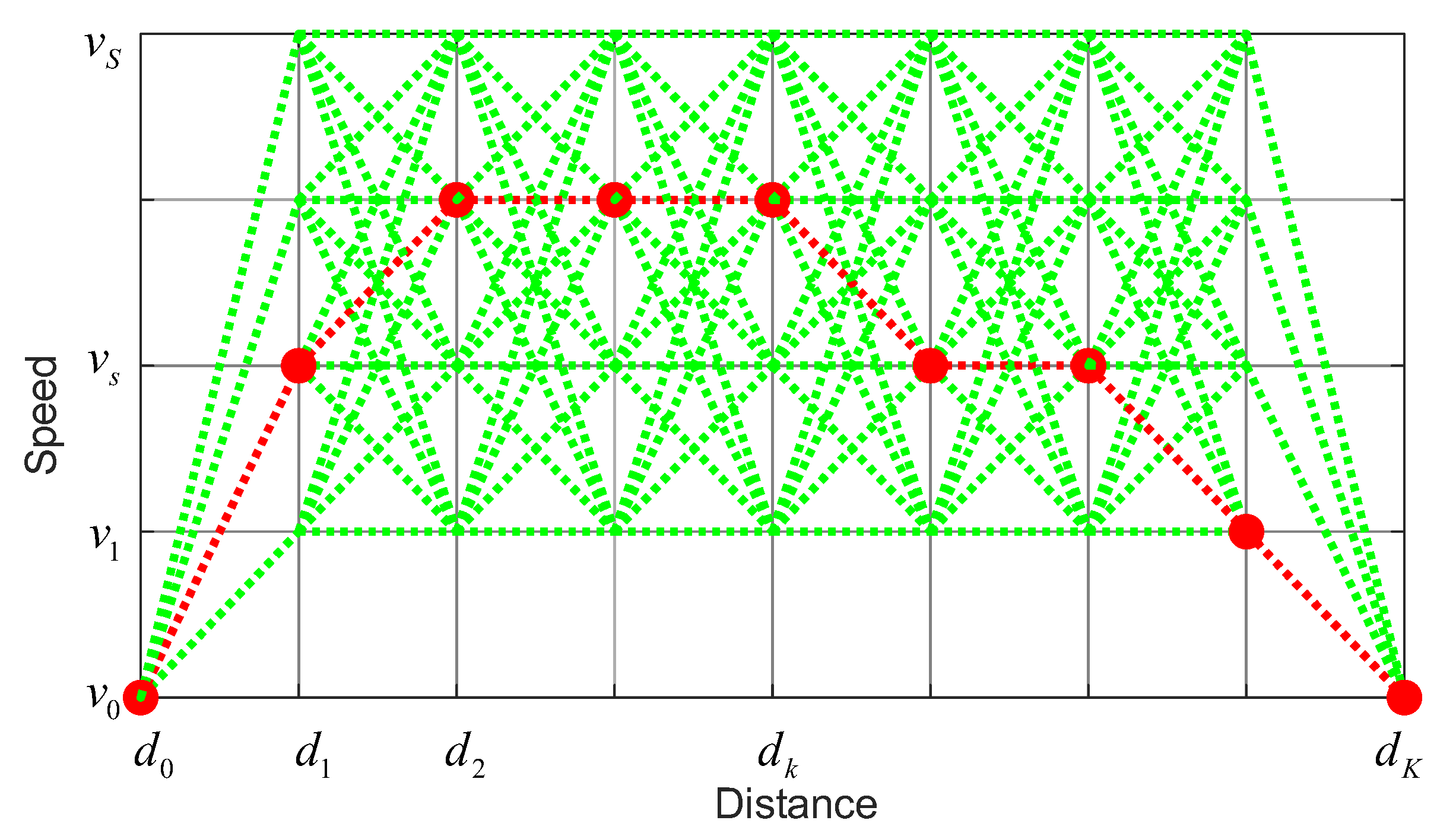
The target distance (dK) and maximum speed (vs) of the running section are shown in Figure 1. Each axis is discretized at regular intervals. We designed a discrete space where the y-axis is the velocity axis and each step is set as a state. The number of velocity-axis nodes is Nv = Vmax/dv. Here, Vmax is the maximum running speed, dv is the interval of discrete speed, and Nd = df/ds is the number of nodes on the distance axis. Further, df is the total distance traveled, and ds is the interval of discrete distance. In this discrete space, the total number of nodes is Nv × Nd, and the number of edges is Nv2 × Nd. Here, the speed at the starting position (d0) and the arrival position (dK) are zero.
The discretization standard applied to the calculation considers various factors, and, first of all, it was selected considering the accuracy of the location measurement during the operation of the train, the resolution of the speed control, and the resolution of the weights. This is because the speed profile of the train is created using the position-based speed value; therefore, even if it is designed with a resolution higher than that, it is impossible to precisely control the speed of the train at the designed position. The location-measurement accuracy of the train on the test route was selected based on 10 m or less, and discrete distance (ds) values were set accordingly; however, it can be adjusted according to the location accuracy of the train under consideration. Here, the running time between nodes is variable according to the moving average speed between nodes when the travel distance between the nodes is fixed. Furthermore, Vmax is determined by the maximum value of the train’s propulsion system. Table 2 presents the parameters used in this study.
- (2)
- Cost allocation for each edge of the node connection
At the edge connecting the two nodes, when ds is constant, the amount of power calculated for each speed change and the time required to move are recorded. In addition, the sum of the weighted values of these two values is recorded. For multiple weights, the cost equal to the number of weights is recorded.
Here, the cost is recorded at each edge connecting the front and rear nodes from the starting point. At this time, the cost is determined using the speed of each node that connects the edges and the movement distance between the nodes. The time (Ti) and energy (Ph) required to move between these two nodes are calculated. Moreover, the acceleration between two adjacent nodes is calculated using Equation (11), and the moving time is obtained using the average-speed (vm), as shown in Equation (10), and the discrete distance (ds) between nodes, as shown in Equation (12).
Then, the energy (Ph) required at this time can be obtained using the force and speed required for moving between nodes, as shown in Equation (13). The weighted cost can be calculated using the obtained time and energy, as shown in Equation (14). In this case, the weight (α) is an array that is obtained by dividing the value between [0,1] into several parts. Each weight can determine the time and energy-ratio allocation ratio. When the weight is zero, the time is minimized, and when the weight is one, the solution can be obtained, such that the energy consumption is minimized. Therefore, if this weight is set to a value between zero and one, the destination arrival time and energy consumption change accordingly. Here, the arrival time is determined according to the proportion of each weight applied to the cost function. According to the optimization cost function in Equation (14), when the weight is 0, it has the fastest arrival time, while when the weight is 1, it has the slowest arrival time. Therefore, each edge is recorded as an array of costs equal to the number of weight decompositions.
where Ek is the cost at the edge with multiple weights that determine the ratio between time and energy. The weight is defined by Equation (15).
The weight interval between 0 and 1 is adjusted by applying an exponential function, as shown in Equation (16), to reduce the duplication of velocity profiles as much as possible. Here, x is equally divided and applied using the desired number of weights.
Here, Pmax and Pmin are the maximum and minimum section energies, respectively, and Tmax and Tmin are the maximum and minimum section travel times, respectively. Pmax and Pmin are, respectively, determined by checking the maximum and minimum values of each Ph value determined between each node using Equation (13) in the node-data-setting stage before optimization. Similarly, Tmax and Tmin are, respectively, determined by checking the maximum and minimum values of the Ti values calculated using Equation (12). Table 3 presents the parameters of the cost function used in this study (Equation (13)).
For an optimization problem with a total of Nd stages, we aim to find the path with the smallest cumulative sum of the stage energy costs Ek, as shown in Equation (17).
- (3)
- Generate the minimum cost and optimal path at each node in the reverse direction
Now, if the cost is determined for all edges in the network connecting each node in the two-dimensional plane for distance and speed, to apply dynamic programming, Equation (18) represents the structure of a typical DP algorithm. It is a mechanism that reduces the computation time by preventing duplicate calculation of cost at each edge. To do this, the calculation is performed starting from the final stage and going backward to the minimum-cost calculation. At each stage, the minimum cost and optimal node are stored, and the optimization is performed until the starting stage. By proceeding with this procedure, the final optimal path can be obtained from the starting stage. In Equation (18), Ek,: is the cost matrix calculated using Equation (14) at the k-th stage, and Jk+1,: is the optimal cost matrix cumulatively calculated from the k+1-th stage to the final stage using Equation (18).
Here, Jk is the minimum cost from the k stage to the final stage, and it is composed of an array with N+1 values that are calculated according to each weight, as shown in Equation (19). Here, Ik consists of an array with N+1 position indexes of the minimum value for each weight, and mincol defines the minimum value for each column in a matrix.
Here, Ek,: is an s (N + 1) matrix corresponding to the cost of the number of weights corresponding to each multiple weight among the costs of each edge connected to node k + 1 in each stage k, and Jk+1,: is an s (N + 1) matrix corresponding to each multiple weight as the matrix of the optimal cost calculated from node k + 1 to the destination. The term s represents the number of states in each stage, that is, the number of nodes on the velocity axis.
Starting from the destination point and proceeding in reverse order, when the minimum cost and the node index are determined at each stage, the optimal node number is recorded, and this process is repeated until the starting point. Equation (23) is the optimal node-index-processing step followed in this process. Here, all starting and ending nodes are excluded because the speed at these nodes is set to zero.
Step K-1: The stage just before the end of the distance axis
Step k: for (1 ≤ k < K − 1),
Among the optimal paths (Pk+1) stored in stage k + 1, the path recorded in the optimal node index (Ik) found in stage k is called. From this value, if the path corresponding to the weight sequence is extracted, as shown in Equation (25), the entire optimal node (Pn) up to stage k + 1 connected with the optimal node (Ik) of stage k can be extracted.
Here, Pn is the minimum-cost path at stage k+1 for each weight, and the optimal path in step k is generated by adding the stage k+1 optimal path (Pn) to the stage k optimal node (Ik), as shown in Equation (26). This process is repeated in the direction of the starting node.
Therefore, in the last stage, stage 1, the cost and the optimal path in Equation (27) are constructed.
Then, the optimal path for all weights considering the starting node is completed using Equation (28).
- (4)
- Speed-profile creation using optimal node
The optimal speed profile using the final node information of Equation (28) is arranged when dv is applied, as shown in Equation (29).
where dv = vk+1 − vk is the interval of discrete speed.
- (5)
- Required time and energy according to the speed profile for each weight
By following the node number obtained in Equation (28) from the starting node, the section time (Ti), the section energy (Ph) recorded in each node, and the total energy used can be obtained.
4. Results and Discussion
This study presents a method for obtaining an optimal solution using the DP algorithm, wherein a cost function with multiple weights is applied. To obtain an optimal train-running speed profile that satisfies the existing travel target time, the process and time of the repeated weight were changed and the calculations were shortened. We, thus, propose a method for calculating the optimal speed profile, the running time, and the energy consumption, which can be simultaneously operated. The train-operation information such as moving distance, gradient, and speed limit used in this study is based on actual Seoul Metropolitan Rapid Transit route operation data. The specifications of the computer used for the calculation are Intel core i5 processor with four cores, a clock speed of 3.4 GHz, and 16 GB RAM of memory.
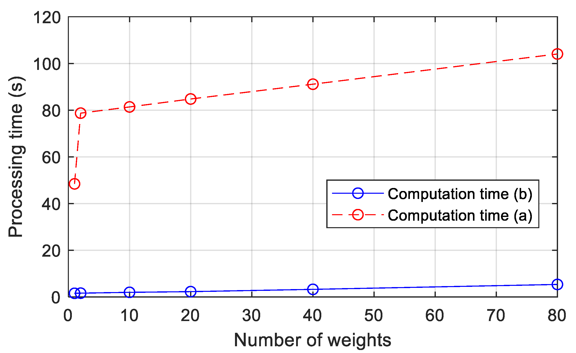
To study the processing performance of the proposed method, the number of weights was increased, and the computation time was checked accordingly. In Table 4, the calculation time (a) is the minimum-cost-search computation time, excluding the cost-setting time of each node and edge in the DP algorithm. The calculation time (b) results from the total computation time, including the cost setting and minimum-cost search of each edge and node in the DP algorithm. Figure 2 displays a plot of the results presented in Table 4. This shows that significantly more time is consumed when setting the cost of the computation space than the time (a) required to find the optimal solution. Here, the case of one weight of the calculation time (a) is the same as the time taken for one calculation in the existing method.
If the conventional algorithm finds the optimal speed profile of the target travel time after only 10 weight corrections [15], according to the total calculation time (b), it will take 10 times the search time, that is, 48.445 × 10 = 484 s. In [15], the tolerance for the target travel time is 0.5 s. Assuming that the computational space is sufficiently discretized and achieves the same purpose as that of the proposed method, the target result can be obtained within two trials. First, 80 weights in the range of 0–1 are applied, and the calculation is performed once. In this result, if there is no target travel time result within the tolerance, the range is limited to the weights of the front and back areas, including the target travel time, and the same calculation is performed by applying 80 redivided weights. Thus, it will be possible to obtain a velocity profile that satisfies the target travel time. In the test results presented in Table 5, the maximum travel-time difference between weights was within 8.6 s. If the calculation space has a sufficient discrete space, and it is calculated using 80 redivided weights within this range of adjacent weights, the target velocity profile within the target tolerance of 0.5 s can be obtained. The number of weight divisions may change according to the desired degree of error. In this case, when the proposed method is applied, the solution can be found in approximately 104 × 2 = 208 s, and multiple velocity profiles can be obtained by a batch-processing method within 1/2 h of the existing method. If this result is integrated as a table, it is possible to immediately apply the desired travel-time speed profile without performing calculations when the target travel time changes, when considering a train operation delay.
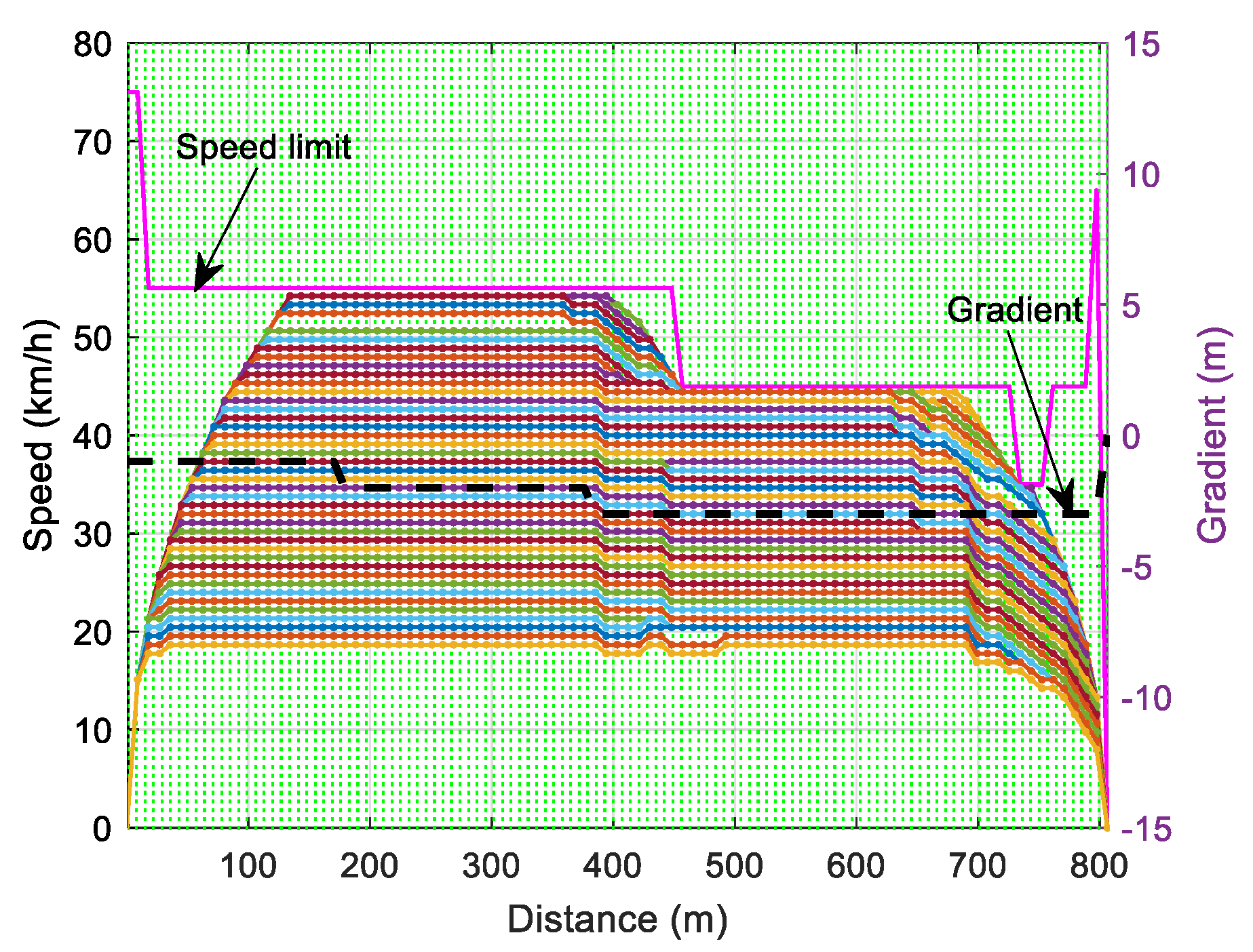
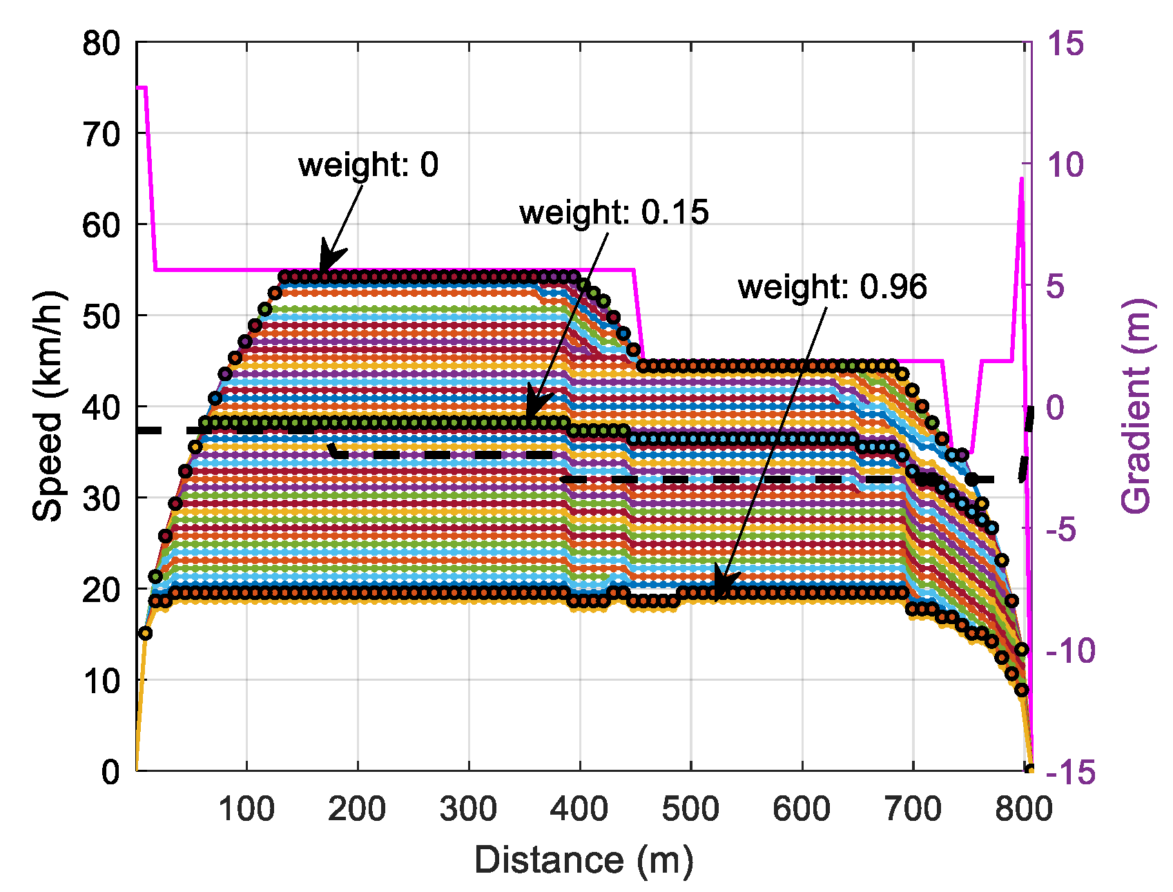
Figure 3 shows each velocity profile generated by applying 80 weights. The total travel distance is 806.25 m, and the maximum speed is 80 km/h. A total of 90 nodes were created for each distance and speed in two-dimensional space. From the results in Table 5, a speed profile that satisfies a minimum travel time of 75.56 s and a maximum travel time of 172.5 s was obtained, according to the section-operation-restriction conditions (slope and speed limit). The minimum travel time is the time required for the operation when the maximum performance (acceleration and deceleration performance) of the train is exhibited under operating constraints such as limited speed, gradient, travel distance, propulsion, and braking performance. The maximum travel time is the time it takes for a train to travel to its destination while consuming minimum energy under operational constraints. From this result, 49 speed profiles without any overlap were obtained, and 31 profiles with the same velocity were created. This result generates the same velocity profile because the resolution of the distance and velocity axis is not sufficiently generated to obtain a different cost. Therefore, to increase the arrival time resolution, it is necessary to increase the number of nodes on the distance and velocity axes, that is, to improve the resolution.
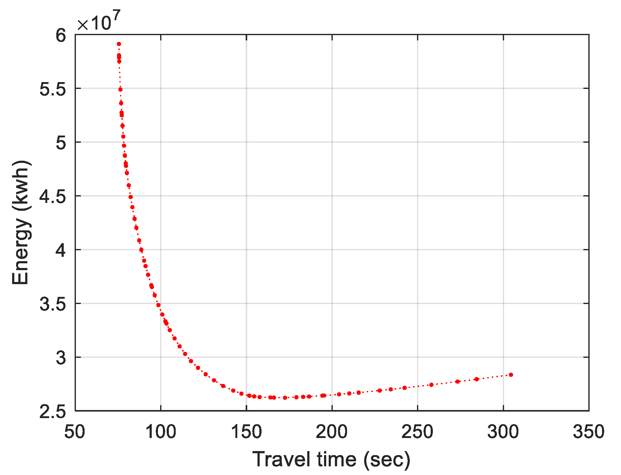
Figure 4 shows the results of the travel time and energy consumption for each weight. The smaller the travel time is, the sharper the energy consumption is. Here, the minimum and maximum times are 75.56 s and 172.5 s, respectively. In the cost-function equation, Equation (14), if the weighting factor 1 with the minimum energy is exceeded, the driving energy is increased again, as shown in Figure 4. This is because of the energy continuously used by the electric equipment in the train, regardless of the driving.
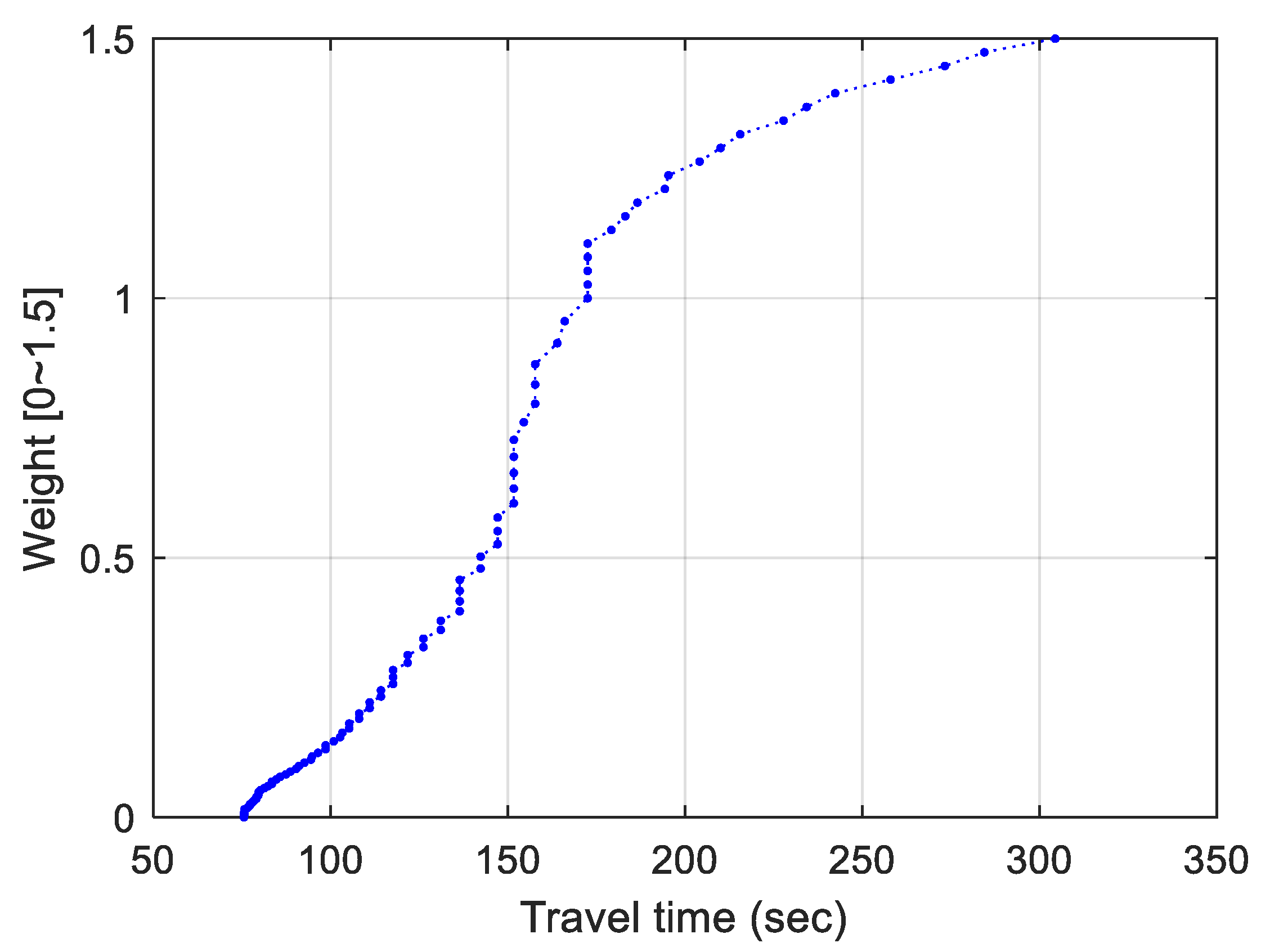
Figure 5 shows the travel time for the applied weights. As shown in the figure, the exact weight is duplicated at some arrival times. When the weight resolution is higher than the node resolution, a duplicate velocity profile with the same arrival time is created. Here, the weight division interval is increased exponentially rather than linearly, and, thus, the velocity profile is evenly created.
Figure 6 shows that three of the split weights, [0, 0.15, 0.96], are applied to the single cost function to check whether the processing result of the DP algorithm with the multi-weighted array processing is consistent with the single-weighted processing result. From the results, it can be confirmed that the results are consistent with each other. In Table 6, the calculation results of each method are compared and presented as quantitative values. This was performed to confirm that each weight could yield the same result. This confirmed that the multi-weighted array’s DP algorithm could be seamlessly calculated.
5. Conclusions
In previous studies, when the DP algorithm was used to obtain the optimal speed profile, given the distance between stations and the target travel time, the cost function was set according to both time and energy. Further, the weight was changed to find the optimal solution that satisfies the target travel time. These calculations were repeated until the target travel time was satisfied. This study proposed a method to reduce the time required to find the optimal solution by shortening the process of repeating weight changes and calculations.
This paper presents the DP algorithm that divides the weights applied to time and energy into several cost functions and arranges them to shorten the time required to obtain the desired solution.
The computation time according to the number of weights applied and the time required to obtain the optimal solution through multi-weight processing were compared with the time required for the approach, wherein single weights are repeatedly changed and calculated. This indicated that multi-weighted computational processing may reduce the time required to find a solution more effectively compared to single-weighted iterative processing. In addition, by processing multiple weights at once and checking the results, it was possible to simultaneously confirm the optimal minimum and maximum travel times and energy required for the relevant section. This result can be used to change and establish an effective train operation plan. In addition, the results of this study can be used to minimize the energy consumption for train operation and maximize the energy efficiency.
Author Contributions
Y.S.B. developed the theoretical basis to apply dynamic programming, carried out the numerical simulation for the implementation of the algorithm, and made important contributions to the discussion of the manuscript. R.G.J. supervised the entire work and provided an understanding of the electric train’s power system in general. All authors have read and agreed to the published version of the manuscript.
Funding
This research was funded by the Research and Development Program through the Development of Autonomous Train Control Core Technology by the Korea Railroad Research Institute, under grant number PK2201B1.
Conflicts of Interest
The authors declare no conflict of interest.
References
- Gu, Q.; Tang, T.; Song, Y. A survey on energy-saving operation of railway transportation systems. Meas. Control 2010, 43, 209–211. [Google Scholar] [CrossRef] [Green Version]
- Milroy, I.P. Aspects of Automatic Train Control. Ph.D Thesis, Loughborough University, Loughborough, UK, 1980. [Google Scholar]
- Chevrier, R.; Marliere, G.; Vulturescu, B.; Rodriguez, J. Multi-Objective Evolutionary Algorithm for Speed Tuning Optimization with Energy Saving in Railway: Application and Case Study; RailRome: Rome, Italy, 2011. [Google Scholar]
- Huang, Y.; Ma, X.; Su, S.; Tang, T. Optimization of Train Operation in Multiple Interstations with Multi-Population Genetic Algorithm. Energies 2015, 8, 14311–14329. [Google Scholar] [CrossRef]
- Fernández-Rodríguez, A.; Cucala, A.P.; Fernández-Cardador, A. An eco-driving algorithm for interoperable automatic train operation. Appl. Sci. 2020, 10, 7705. [Google Scholar] [CrossRef]
- Lu, S.; Hillmansen, S.; Ho, T.K.; Roberts, C. Single-Train Trajectory Optimization. IEEE Trans. Intell. Transp. Syst. 2013, 14, 743–750. [Google Scholar] [CrossRef]
- Huang, Y.; Yang, C.; Gong, S. Energy Optimization for Train Operation Based on an Improved Ant Colony Optimization Methodology. Energies 2016, 9, 626. [Google Scholar] [CrossRef] [Green Version]
- Kim, K.; Chien, S.I.J. Optimal Train Operation for Minimum Energy Consumption Considering Track Alignment, Speed Limit, and Schedule Adherence. J. Transp. Eng. 2011, 137, 665–674. [Google Scholar] [CrossRef]
- Xie, T.; Wang, S.; Zhao, X.; Zhang, Q. Optimization of Train Energy-Efficient Operation Using Simulated Annealing Algorithm. In Intelligent Computing for Sustainable Energy and Environment; Li, K., Li, S., Li, D., Niu, Q., Eds.; Springer: Berlin/Heidelberg, Germany, 2013; pp. 351–359. [Google Scholar]
- Miyatake, M.; Ko, H. Optimization of train speed profile for minimum energy consumption. IEEJ Trans. Electr. Electron. Eng. 2010, 5, 263–269. [Google Scholar] [CrossRef]
- Ozatay, E.; Onori, S.; Wollaeger, J.; Ozguner, U.; Rizzoni, G.; Filev, D.; Michelini, J.; Di Cairano, S. Cloud-based velocity profile optimization for everyday driving: A dynamic-programming-based solution. IEEE Trans. Intell. Transp. Syst. 2014, 15, 2491–2505. [Google Scholar] [CrossRef]
- Ko, H.; Koseki, T.; Miyatake, M. Application of dynamic programming to optimization of running profile of a train. In Computers in Railways IX; WIT Press: Southampton, UK, 2004; pp. 103–112. [Google Scholar]
- Miyatake, M.; Haga, H.; Suzuki, S. Optimal speed control of a train with on-board energy storage for minimum energy consumption in catenary free operation. In Proceedings of the 2009 13th European Conference on Power Electronics and Applications, Barcelona, Spain, 8–10 September 2009. [Google Scholar]
- Mensing, F.; Trigui, R.; Bideaux, E. Vehicle trajectory optimization for application in ECO-driving. In Proceedings of the 2011 IEEE Vehicle Power and Propulsion Conference, Chicago, IL, USA, 6–9 September 2011; pp. 1–6. [Google Scholar] [CrossRef]
- Mensing, F. Optimal Energy Utilization in Conventional, Electric and Hybrid Vehicles and Its Application to Eco-Driving. Ph.D. Dissertation, INSA Lyon, Villeurbanne, France, 2013. [Google Scholar]
- Pröhl, L.; Aschemann, H.; Palacin, R. The Influence of Operating Strategies regarding an Energy Optimized Driving Style for Electrically Driven Railway Vehicles. Energies 2021, 14, 583. [Google Scholar] [CrossRef]
- Mensing, F.; Bideaux, E.; Trigui, R.; Tattegrain, H. Trajectory optimization for eco-driving taking into account traffic constraints. Transp. Res. D Transp. Environ. 2013, 18, 55–61. [Google Scholar] [CrossRef]
- Themann, P.; Bock, J.; Eckstein, L. Optimisation of energy efficiency based on average driving behaviour and driver’s preferences for automated driving. IEEE Trans. Intell. Transp. Syst. 2015, 9, 50–58. [Google Scholar] [CrossRef]
- Monastyrsky, V.V.; Golownykh, I.M. Rapid computation of optimal control for vehicles. Transp. Res. Part B Methodol. 1993, 27, 219–227. [Google Scholar] [CrossRef]
- Naldini, F.; Pellegrini, P.; Rodriguez, J. Real-Time Optimization of Energy Consumption in Railway Networks. Transp. Res. Procedia 2022, 62, 35–42. [Google Scholar] [CrossRef]
- Bosquet, R.; Vandanjon, P.; Coiret, A.; Lorino, T. Model of High-Speed Train Energy Consumption. World Acad. Sci. J. Eng. Technol. 2013, 78, 1912–1916. [Google Scholar]
- Rocha, A.; Araújo, A.; Carvalho, A.; Sepulveda, J. A New Approach for Real Time Train Energy Efficiency Optimization. Energies 2018, 11, 2660. [Google Scholar] [CrossRef]
- Davis, W.J. Tractive Resistance of Electric Locomotives and Cars. Gen. Electr. Rev. 1926, 29, 685–708. [Google Scholar]
- Partab, H. Modern Electric Traction; Natraj Offset Printer (Delhi); Gagan Kapur for Dhanpat Rai& Co.(P) LTD Educational and Technical Publisher: Delhi, India, 2010. [Google Scholar]
- Bellman, R.; Kalaba, R. Dynamic Programming and Modern Control Theory; Academic Press: New York, NY, USA, 1964. [Google Scholar]
Figure 1.
Speed profile according to dynamic program algorithm. (Green: possible paths, Red: optimal path).
Figure 1.
Speed profile according to dynamic program algorithm. (Green: possible paths, Red: optimal path).

Figure 2.
Processing time for number of weights.

Figure 3.
Speed profiles by DP with multiple weights.

Figure 4.
Pareto curve for multiple weights between energy consumption versus time.

Figure 5.
Results of weight versus time.

Figure 6.
Comparison of multi-weighted and single-weighted DP results.


Table 1.
Train parameters.
| m (kg) | 168,000 |
| FacMax (kN) | 240.05 |
| FdcMax (kN) | −165 |
| Vac (km/h) | 35 |
| Vdc (km/h) | 40 |
| ar | 1.867 |
| br | 0.0359 |
| cr | 0.000745 |
Table 2.
Discretization and parameters for dynamic programming.
| Total Travel Distance (m) | Max Speed (km/h) | ds (m) | dv (m/s) | Number of Distance Axis Nodes (Nd) | Number of Velocity Axis Nodes (Nv) |
|---|---|---|---|---|---|
| 806.25 | 80 | 8.96 | 0.25 | 90 | 90 |
Table 3.
Parameters of the cost function.
| Pmax (J) | Pmin (J) | Tmax (s) | Tmin (s) |
|---|---|---|---|
| 5 × 10⁶ | 11,027 | 80 | 0.4 |
Table 4.
Processing result according to number of weights.
| Number of Weights | 1 | 2 | 10 | 20 | 40 | 80 |
|---|---|---|---|---|---|---|
| Computation time (s) (a) | 1.568 | 1.631 | 1.985 | 2.284 | 3.260 | 5.359 |
| Computation time (s) (b) | 48.445 | 78.732 | 81.390 | 84.794 | 91.130 | 104.074 |
Table 5.
Results of speed profiles obtained for multiple weights.
| Index | Weighting Factor | Travel Time (s) | Energy (kwh) |
|---|---|---|---|
| 1 | 0 | 75.56 | 59,129.12 |
| 2 | 0 | 75.56 | 59,129.12 |
| 3 | 0 | 75.56 | 59,129.12 |
| 4 | 0 | 75.56 | 59,129.12 |
| 5 | 0.01 | 75.6 | 58,516.07 |
| ⋮ | ⋮ | ⋮ | ⋮ |
| 76 | 0.83 | 154.49 | 26,338.68 |
| 77 | 0.87 | 157.7 | 26,279.28 |
| 78 | 0.91 | 157.7 | 26,279.28 |
| 79 | 0.96 | 163.94 | 26,239.95 |
| 80 | 1 | 172.5 | 26,218.99 |
Table 6.
Comparison of single-weight and multi-weight calculation results.
| Weights | Travel Time (Single) (s) | Travel Time (Multi) (s) | Energy (Single) (kwh) | Energy (Multi) (kwh) |
|---|---|---|---|---|
| 0 | 75.56 | 75.56 | 59,129.12 | 59,129.12 |
| 0.146262 | 100.88 | 100.88 | 33,955.46 | 33,955.46 |
| 0.955694 | 166.05 | 166.05 | 26,232.48 | 26,232.48 |
Publisher’s Note: MDPI stays neutral with regard to jurisdictional claims in published maps and institutional affiliations. |
© 2022 by the authors. Licensee MDPI, Basel, Switzerland. This article is an open access article distributed under the terms and conditions of the Creative Commons Attribution (CC BY) license (https://creativecommons.org/licenses/by/4.0/).
Share and Cite
MDPI and ACS Style
Byun, Y.S.; Jeong, R.G. Optimization of Driving Speed of Electric Train Using Dynamic Programming Based on Multi-Weighted Cost Function. Appl. Sci. 2022, 12, 12857. https://doi.org/10.3390/app122412857
AMA Style
Byun YS, Jeong RG. Optimization of Driving Speed of Electric Train Using Dynamic Programming Based on Multi-Weighted Cost Function. Applied Sciences. 2022; 12(24):12857. https://doi.org/10.3390/app122412857
Chicago/Turabian StyleByun, Yeun Sub, and Rag Gyo Jeong. 2022. "Optimization of Driving Speed of Electric Train Using Dynamic Programming Based on Multi-Weighted Cost Function" Applied Sciences 12, no. 24: 12857. https://doi.org/10.3390/app122412857
Note that from the first issue of 2016, this journal uses article numbers instead of page numbers. See further details here.