A Comparative Study for Some Mathematical Models of Epidemic Diseases with Application to Strategic Management

Abstract

A local performance of the SIR model on actual data is introduced. A good approximation of the SIR model parameters in Saudi Arabia during a period of 275 days (the first of April 2020 to the end of December 2020) is determined. The parameters are estimated from the recorded data and used to predict the values in the next subsequent period. The performance of the standard fourth order Runge–Kutta method is considered for the classical SIR models over different periods. A comparison of the recorded data and the predicted values during the considered period illustrated the effectiveness of the treatment. The mathematical properties and initial conditions are considered within the estimated parameter values. It is shown that lockdown and social distance attitudes effectively controlled the spread of the disease. The maximum number of daily active infected cases is 63,026, and occurs in July and this agrees with the calculated values. To make the graphs representable, we considered a fixed closed population, the effective sample during the considered period of size N = 400,000 only (represents only 1% of the overall population susceptible, this must be associated, with great thanks, to the authorities in KSA).

1. Introduction

There is no life without disease. Therefore, over the years, people have spent a lot of effort and financial and moral support to control the spread of diseases or avoid their side effects. The side effects of the spread of diseases vary from health damage to psychological impacts, social impacts, and economic impacts. With the scientific and technological developments of humankind, studies of problems and setting up scenarios for dealing with them have become one of the most important strategies. Accordingly, nations can avoid the serious side effects of such problems. Among the most prominent of these problems is the spread of infectious diseases, whether they are bacterial or viral. The category of epidemic diseases is one of the most difficult and dangerous disease types that civilization has faced. The dynamics of transmission of almost all infectious diseases are known, so the establishment of good mathematical models for the spread of infectious diseases are reachable tasks [1,2]. Mathematical models are considered among the most major pre-studies that can be used in developing strategies for dealing with epidemics.

Mathematical models, in principle, fall into two categories:

First, the statistical models are those that monitor reality in all its details, but their future role is restricted, their accuracy is difficult to be estimated, and they are judged by realistic measurements, which usually suffer from exactness. Therefore, the role of statistical models is limited in strategic planes despite their essential responsibility in determining the model parameters for any model type [2,3].

Second, mathematical models are based on fixed, unquestionably physical, mathematical laws and facts. Mostly, they are related to rates of change, and therefore they are often differential or integrodifferential equations in different forms. Now there are many mathematical models. All the models can give acceptable results, provided that are used in an appropriate manner, and their parameters are rightly determined [1,2].

Epidemiological mathematical models are a remarkable type of population model, especially the well-known prey-predator model, which represents the struggle of survival. The concepts of prey and predator are the cornerstone of the mathematical models of many biological studies. The following system of two nonlinear ordinary differential equations (ODEs), is known as Volterra’s prey-predator model.

$$\begin{array}{ccc}\frac{dx}{dt}\hfill & =& \mu x-\nu xy;\mu ,\nu >0,\hfill \\ \frac{dy}{dt}\hfill & =& -\rho y+\sigma xy;\rho ,\sigma >0,\hfill \end{array}x\left(0\right)=c_{1}andy\left(0\right)=c_2.$$

(1)

To discuss the solution of such systems, one must determine the parameters of the model $\mu ,\nu ,\rho ,\sigma ,c_1$ and $c_2$. Determination of the parameters of the model is the most important step in the mathematical treatment; wrong values of even only one of the parameters can destroy all the results.

Although this model is one of the elementary models described in calculus books, it contains all the characteristics of the most complicated models (ODE models). One can see, from the first equation, the exponential behavior of $x\left(t\right)$ in the case of $\nu =0$, also the role of $\nu$ in controlling the exponential increase in $x\left(t\right)$. Furthermore, one can see the exponential decay in $y\left(t\right)$ from the second equation, and the role of $\sigma$ to control the exponential decay in $y\left(t\right)$ [2,4,5].

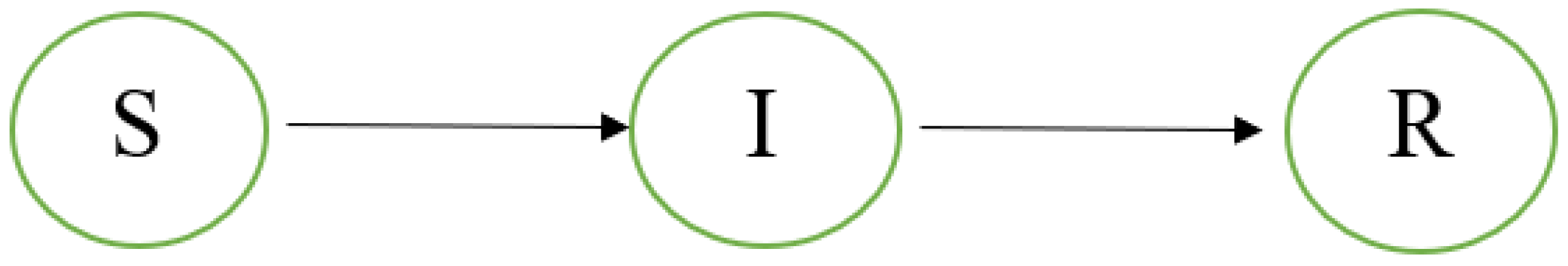
Now we consider one of the simplest, oldest mathematical models used in the epidemic diseases cited in many publications and can be considered as the extension of the prey-predator model, the SIR model introduced by Kermack and McKendrick in 1927–1933.

The model consists of a system of three coupled nonlinear ordinary differential equations for the unknowns $S\left(t\right)$ (susceptible), $I\left(t\right)$ (infective), and $R\left(t\right)$ (removable) Figure 1, with $N=S\left(t\right)+I\left(t\right)+R\left(t\right)$ a fixed closed population under consideration, as follows:

$$\begin{array}{ccc}{S}^{{}^{\prime }}\left(t\right)& =& -\beta SI,\hfill \\ I^{{}^{\prime }}\left(t\right)& =& \beta SI-\alpha I,\hfill \\ R^{{}^{\prime }}\left(t\right)& =& \alpha I,\hfill \\ S\left(0\right)& =& S_0,I\left(0\right)=I_0,R\left(0\right)=R_0.\hfill \end{array}$$

(2)

Mathematically, the initial stage at $t=0$ can be taken as any point in available trusted data. The determination of the nonnegative parameters of the model $\beta ,\alpha ,S_0,I_0$ and $R_0$ is the most difficult and critical step in using this model. It is easy to see the increasing behavior of $R\left(t\right)$ and the decreasing behavior of $S\left(t\right)$ due to the sign of the first-order derivative. The behavior of $I\left(t\right)$ is the effective part of any explanation. The peak occurs when $\alpha =\beta S$ [1,2]. Due to the nonlinearity in such systems, methods for solution are directed towards approximate and numerical techniques [4,5,6,7,8,9]. At the heart of the numerical methods for such systems are the Runge–Kutta (RK) methods, especially the fourth order. The parameters $\alpha$ and $\beta$ are known as the recovery coefficient and the transmission coefficient, respectively, [1,2].

There are many trials to upgrade the SIR model (2), but more parameters are included and other scientific concepts such as fractional calculus or stochastic behavior’s must be considered [10,11,12]. Among them, some authors [13,14] considered the relaxation of the assumption of bilinearity of the incidence rate $\beta SI$ to cover different dynamical behaviors. In 2012, Mickens [14] assumed that the interaction terms that appear in the SIR model can take the form of square root and introduced a new SIR model of the form:

$$\begin{array}{ccc}{S}^{{}^{\prime }}\left(t\right)& =& -{\beta }^{*}\sqrt{SI},\hfill \\ I^{{}^{\prime }}\left(t\right)& =& {\beta }^{*}\sqrt{SI}-{\alpha }^{*}\sqrt{I},\hfill \\ R^{{}^{\prime }}\left(t\right)& =& {\alpha }^{*}\sqrt{I},\hfill \\ S\left(0\right)& =& S_0,I\left(0\right)=I_0,R\left(0\right)=R_0.\hfill \end{array}$$

(3)

There is no doubt that the models (2) or (3) can be applied to develop comprehensive treatment scenarios and strategic plans at the beginning of an outbreak of any disease, providing a good estimation of the available data. As a result of the developments of information technology and modern methods of communication, health authorities all over the world have been able to monitor the data and make it available for use, serving humanity by developing methods for preserving human beings in general.

Each model contains five parameters: three of them are just the initial values $S_0,I_0$, and $R_0$, and these values can be easily obtained from the daily data available for each case study. The other two parameters $\beta$ and $\alpha$ for the model (2) or ${\beta }^{*}$ and ${\alpha }^{*}$ for the model (3) can be determined from the available data. The reliability of the obtained solutions depends on the accuracy of the determined values for the parameters as well as the method of solution [15,16,17].

Our main task in this work is to adopt the use of simple mathematical models and the real data available to generate good approximate values to the recorded real data so reliable prediction of the spread of the epidemic disease can be analyzed. Therefore, strategic plans of the management of situates can be introduced with high confidence. It is seen that the use of models (2) and (3) depends on the determination of accurate values of the parameters ($\beta$ and $\alpha$ or ${\beta }^{*}$ and ${\alpha }^{*}$) and on using an efficient and reliable method of solution.

In this work, we propose the use of the SIR model in a local way unlike what was used previously. Furthermore, we determine the parameter values from the actual data through mathematical treatment with high credibility (integration technique) unlike what was used previously (differentiation or fitting techniques).

Due to the behavior of the data for daily infected cases, which appears in Figure 2 (cusp values), it is recommended to determine the parameters through numerical integration techniques rather than any other approaches, and this will be adopted in this work. We recommend the WHO dashboard for the actual data [18].

No one can deny the role of modern systems and methods of scientific computing in dealing with models of epidemiological diseases, as they need to deal continuously with large data.

2. Materials and Methods

It is generally accepted that the spread of epidemic diseases is a short-term case [1,2]. Therefore, the use of the data must be adopted to short time scales, it is suggested to restrict the use of the mathematical models to short time periods, so the updated parameter values can be more reliable.

The initial values $I_0$ and $R_0$ are taken from the recorded actual data. The most effective value of the implementation is the size of N and accordingly $S_0$ $(S_0+I_0+R_0=N)$. Usually, N is chosen to be the overall population. When the size N is very large in comparison with actual data $I\left(t\right)$ or $R\left(t\right)$, N can be chosen as significant percentage of the overall size of the population (rescaling the coordinate axes) to make graphs and results representable. After many computational experiments N is chosen to be $1\%$ of the populations in the Kingdom of Saudi Arabia (N = 400,000). 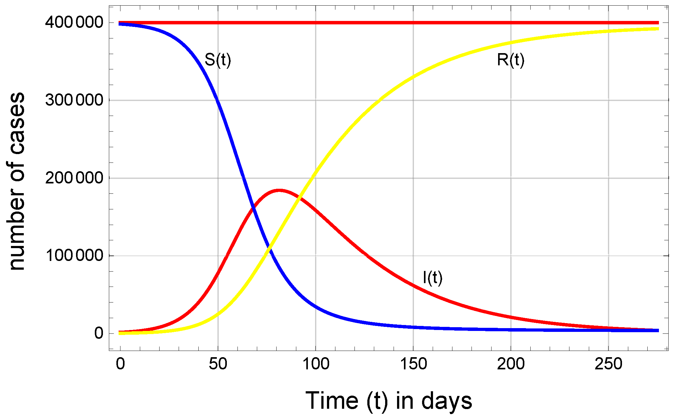Accordingly, $S_0=N-I_0-R_0$, and the time required to transfer most of the population in $S_0$ to $R\left(t\right)$ to match the general behaviors of epidemic as in Figure 3 is approximately 275 days. May other researchers take different values for N. Accordingly, different values for the parameter $\beta$ can be determined. As our case the peak of $I\left(t\right)$ was expected to be in July 2020 so N can be taken in the range from $0.5\%$ up to $1.0\%$ (200,000 to 400,000).

2.1. Reformulation of the Mathematical Models

The short time scale forms of the models (2) and (3) can be written in a more practical form as:

$$\begin{array}{ccc}{S}^{{}^{\prime }}\left(t\right)& =& -{\beta }_{c}SI,\hfill \\ I^{{}^{\prime }}\left(t\right)& =& {\beta }_{c}SI-{\alpha }_{c}I,\hfill \\ R^{{}^{\prime }}\left(t\right)& =& {\alpha }_{c}I,\hfill \\ S\left(0\right)& =& S_0,I\left(0\right)=I_0,R\left(0\right)=R_0.\hfill \end{array}$$

(4)

and,

$$\begin{array}{ccc}{S}^{{}^{\prime }}\left(t\right)& =& -{\beta }_c^{*}\sqrt{SI},\hfill \\ I^{{}^{\prime }}\left(t\right)& =& {\beta }_c^{*}\sqrt{SI}-{\alpha }_c^{*}\sqrt{I},\hfill \\ R^{{}^{\prime }}\left(t\right)& =& {\alpha }_c^{*}\sqrt{I},\hfill \\ S\left(0\right)& =& S_0,I\left(0\right)=I_0,R\left(0\right)=R_0.\hfill \end{array}$$

(5)

This form enables us to update the parameter values continuously and avoid the accumulation of errors for long-term periods. Furthermore, this form enables the applicant to exclude periods with extreme attitudes, such as those occurring at the beginning of the coronavirus or any new diseases. Where ${\alpha }_c,{\beta }_c,{\alpha }_c^{*}$ and ${\beta }_c^{*}$ are the values of the model parameters of the short time period under consideration.

2.2. Determination of the Parameters of the SIR Model

Good methods alone never resolve any problem, but bad or unsuitable ones can make matters worse. The essential part of using epidemic mathematical models is the use of proper parameter values. The parameter values affect not only the unknown calculated values of the model but also the mathematical properties of the model itself [15,17]. To obtain suitable and accurate values of the parameters, our treatment focuses on the model (4). Adding the first two equations of the model (4) and integrating the resultant equation along fixed time period $[t_m,t_n]$, one obtains:

$${\int }_{t_m}^{t_n}{(S\left(t\right)+I\left(t\right))}^{{}^{\prime }}dt=-{\int }_{t_m}^{t_n}{\alpha }_{c}Idt,$$

(6)

$$S\left(t_n\right)+I\left(t_n\right)-S\left(t_m\right)-I\left(t_m\right)=-{\int }_{t_m}^{t_n}{\alpha }_{c}Idt.$$

(7)

Using the assumption, $S\left(t\right)+I\left(t\right)+R\left(t\right)=N$, one finds

$$R\left(t_n\right)-R\left(t_m\right)={\alpha }_c{\int }_{t_m}^{t_n}I\left(t\right)dt,$$

(8)

which is compatible with the third equation, integrating the first equation of the system 4 over the time period $[t_m,t_n]$.

$${\int }_{t_m}^{t_n}\left(\frac{S^{{}^{\prime }}\left(t\right)}{S\left(t\right)}\right)dt=-{\int }_{t_m}^{t_n}{\beta }_{c}Idt,$$

(9)

$$ln\left(\frac{S\left(t_m\right)}{S\left(t_n\right)}\right)={\beta }_c{\int }_{t_m}^{t_n}I\left(t\right)dt.$$

(10)

According to formulas (8) and (10), one can determine the local values ${\alpha }_c$, the local recovery coefficient and ${\beta }_c$, the local transmission coefficient corresponding to the considered period from the daily data on active cases published by the WHO Dashboard [18], and represented in Figure 2 if a good approximation of the integral ${\int }_{t_m}^{t_n}I\left(t\right)dt$, appears in the right hand side of both (8) and (10) is calculated. The data on active cases from day 1 up to day 11, are used, for each month to calculate a good approximation of the integral ${\int }_{t_1}^{t_{11}}I\left(t\right)dt$, $(m=1$ and $n=11)$ many numerical techniques can be used, the simplest form is the trapezoidal rule [4].

$${\int }_{t_1}^{t_{11}}I\left(t\right)dt=\frac{1}{2}\{(I_1+I_{11})+2(I_2+I_3+...+I_{10})\},$$

(11)

where $t_i$ denotes the day i of the month under consideration. Therefore, the parameter values calculated according to this approach for the Saudi Arabia region are given in

Table 1. Total number (T.N.) of confirmed cases, T.N. of recover cases, T.N. of deaths.

Month	T. N. Conf.	T. N. Rec.	T. N. Dea.	$\mathsf{\alpha }$	$\mathsf{\beta }$ ∗ ${10}^{-7}$	Recovery Day’s
April	21,190	2998	152	0.0234	2.764	43
May	62,508	59,279	341	0.0374	1.858	27
June	105,562	68,324	1146	0.059	3.565	17
July	85,082	104,892	1217	0.055	3.104	18
August	39,867	55,138	1031	0.0429	2.901	23
September	18,833	28,358	871	0.0483	4.851	21
October	12,677	14,688	634	0.056	6.828	17
November	10,078	12,960	494	0.060	10.742	17
December	5381	7051	327	0.0773	12.009	13

. From formula (8) the value of ${\alpha }_c$ depends only on the actual recorded data $I\left(t\right)$ and $R\left(t\right)$ not on the selected value N.

The standard recovery time for corona virus COVID-19 [16], during this period is approximately $1/\alpha =14$, which was achieved in December 2020 as shown in Table 1.

2.3. Numerical Performance of the SIR Mathematical Model

The above-mentioned SIR model (4) and (5) can be seen as a special case of the following abstract form:

$$\frac{d{y}_i}{dt}=f_i(t,y_1,y_2,y_3),i=1,2,3.$$

(12)

Subject to the initial conditions

$$y_1\left(t_o\right)=S_0,y_2\left(t_o\right)=I_0,y_3\left(t_o\right)=R_0.$$

(13)

The fourth order Runge–Kutta method is a standard technique used for solving such systems or even comparing with any other newly developed method [4,19] taking the form:

$$y_{i,n+1}=y_{i,n}+\frac{1}{6}(k_{i1}+2k_{i2}+2k_{i3}+k_{i4})i=1,2,3,n=0,1,2,\cdots ,$$

(14)

where,

$$\begin{array}{ccc}{k}_{i1}& =& h{f}_i(t_n,y_{1,n},y_{2,n},y_{3,n}),\\ k_{i2}& =& h{f}_i(t_n+\frac{h}{2},y_{1,n}+\frac{k_{11}}{2},y_{2,n}+\frac{k_{21}}{2},y_{3,n}+\frac{k_{31}}{2}),\\ k_{i3}& =& h{f}_i(t_n+\frac{h}{2},y_{1,n}+\frac{k_{12}}{2},y_{2,n}+\frac{k_{22}}{2},y_{3,n}+\frac{k_{32}}{2}),\\ k_{i4}& =& h{f}_i(t_n+h,y_{1,n}+k_{13},y_{2,n}+k_{23},y_{3,n}+k_{33}),\end{array}$$

(15)

where $i=1,2,3$.

The values of $y_1\left(t\right)$ correspond to those of $S\left(t\right)$, $y_2\left(t\right)$ corresponds to those of $I\left(t\right)$, $y_3\left(t\right)$ corresponds to those of $R\left(t\right)$, and $f_i(t,y_1,y_2,y_3)$ corresponds to the right hand side of equation i, in the system (4) or (5). The numerical experiments of model (4) for which the parameters $\alpha ,\beta$ given in Table 1 and

Table 2. Parameters, symbols and their description.

Symbol	Description
$\mu$	The growth rate of Prey.
$\rho$	The decay rate of the predator.
$\nu$, $\sigma$	Bilinear incidence rate of transmission.
$S\left(t\right)$	Susceptible cases at time t, it is the total size of the sample after removing
	the accumulative number of infected cases.
$I\left(t\right)$	Total number of active infected cases at time t.
$R\left(t\right)$	Removed cases of type (death, recovered, ⋯), at time t
N	Fixed size of the study at any time, the sum of all cases at any time
	$S\left(t\right)+I\left(t\right)+R\left(t\right)=N.$
$\alpha$, ${\alpha }^{*}$	It is the transmission coefficient from $I\left(t\right)$ to $R\left(t\right)$,
	for the SIR model it is the recovery coefficient.
$\beta$, ${\beta }^{*}$	It is the transmission coefficient from S(t) to I(t).

will be considered.

3. Results

Epidemic models are designed for applications along short time periods [20]. The reinfection attitudes have limited effects over short time periods. The SIR models give good scenarios about the behavior of the components of the influenza diseases “COVID-19” ($S\left(t\right)$ and $R\left(t\right)$), as noticed from case studies performed on different regions [3,21,22,23,24]. The numerical outcomes of the SIR models suffer from low accuracy when used over long time intervals due to interaction and accumulation of errors as shown in Table 1 and Figure 3, Figure 4, Figure 5, Figure 6 and Figure 7. There are other factors that have fixed effects on the components of the model, like death or reinfection factors, so they have limited impacts on the behavior of the solution (decreasing or increasing) along short time periods [23]. The determination of the parameters in the SIR models depends on the empirical data and on the accuracy of the techniques used. The values of the parameters have their influence on the calculated solutions, so it is recommended to upgrade the parameter values continuously as we did. Due to the confidence and accuracy of numerical integration techniques in comparison with numerical differentiation approaches, the calculated parameter values shown in Table 1 are highly acceptable (numerical integration techniques control the rapid changes around cusp values). The results of using the Runge–Kutta method in Equations (14) and (15) are summarized as follows:

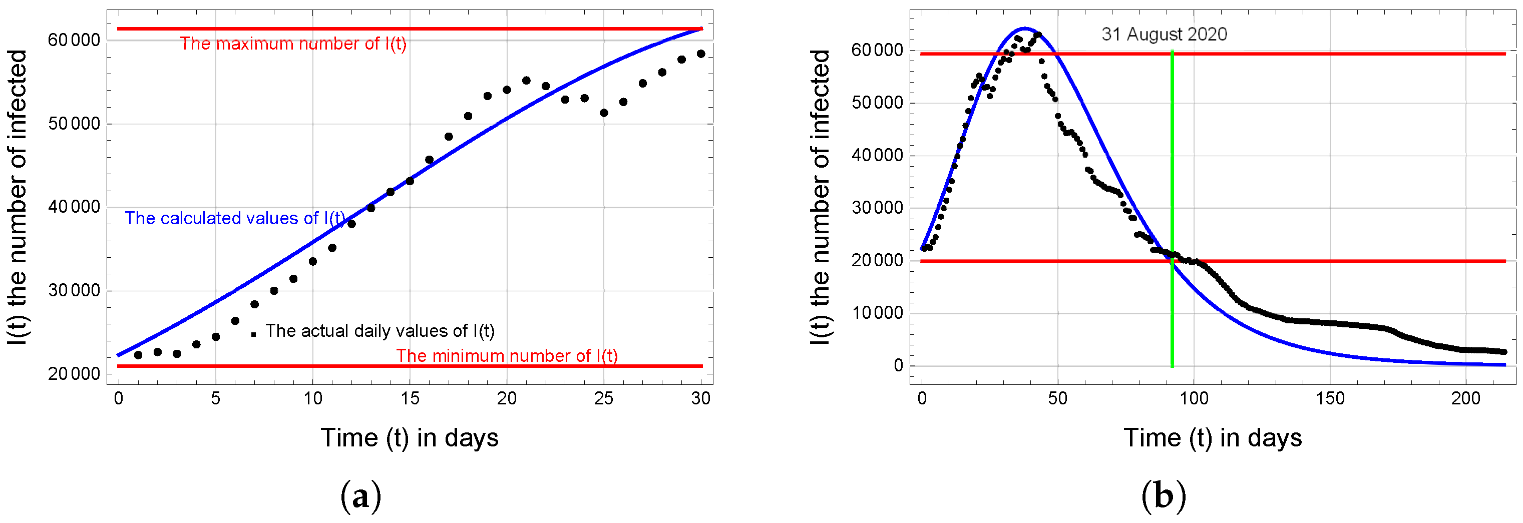
Figure 3 illustrates the calculated components of the SIR model along the overall period from the first of April to the end of December 2020, with the parameters calculated according to April data as in Table 1. It is shown that the maximum active infected cases will be more than 180,000 and it will occur at day 82 from the initial day (21 June) which does not agree with the real data in Figure 2 (the maximum active infected cases will be approximately $63,200$ and it will occur at day 103 from the initial day (12 July)). 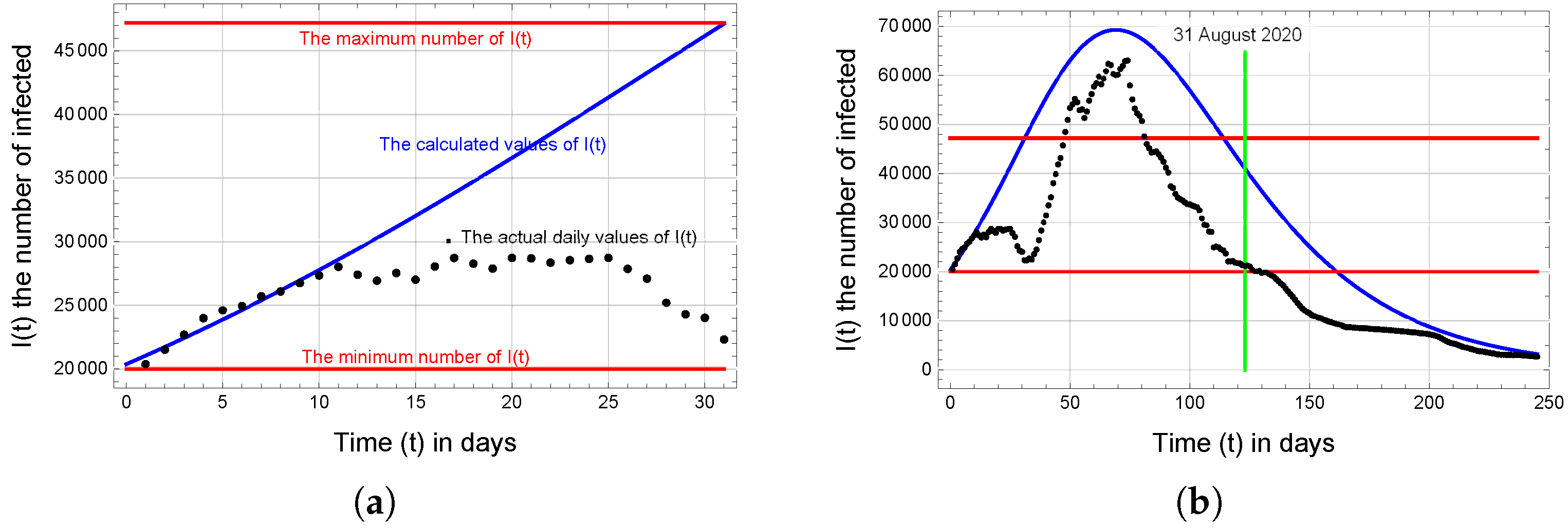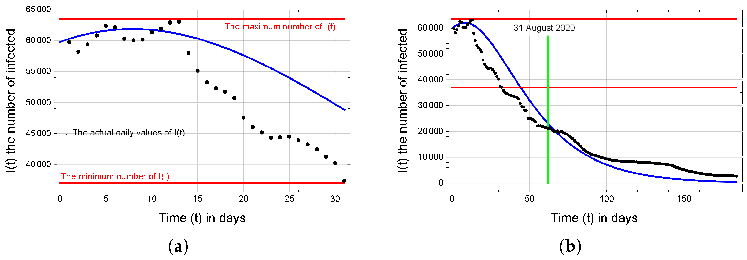Figure 4a illustrates that the number of active infected cases is increasing and Figure 4b illustrates the behavior of the active infected cases along the overall period from the first day of May to the end of December 2020, with the parameters calculated according to May data as in Table 1. It is shown that the maximum active infected cases will be less than 70,000 and it will occur at day 70 from the first day of May (10 July) which tends toward the real situations in Figure 2 (the maximum active infected cases will be approximately 63,200, and it will occur at day 103 of the initial day (12 July)). Figure 5a illustrates that the number of active infected cases is increasing and Figure 5b illustrates the behavior of the active infected cases along the overall period from the first day of June to the end of December 2020, with the parameters calculated according to June’s data as in Table 1. It is shown that the maximum active infected cases will be less than 70,000, and it will occur at day 70 from the first day of May (10 July), which tends toward the real situations in Figure 2 (the maximum active infected will be approximately 63,000, and it will occur at day 38 from the first day of June (8 July)). Figure 6a illustrates that the number of active infected cases reaches its maximum at day 9 from the first day of July and then decreases, and Figure 6b illustrates the behavior of the active infected cases along the overall period from the first day of July to the end of December 2020, with the parameters calculated according to July data as in Table 1. It is shown that the maximum number of active infected cases will be less than 63,200, and it will occur at day 9 of the first day of July (9 July), which tends toward the real situations in Figure 2 (the maximum active infected cases will be approximately 63,000, and it will occur at day 38 from the first day of June (8 July)). 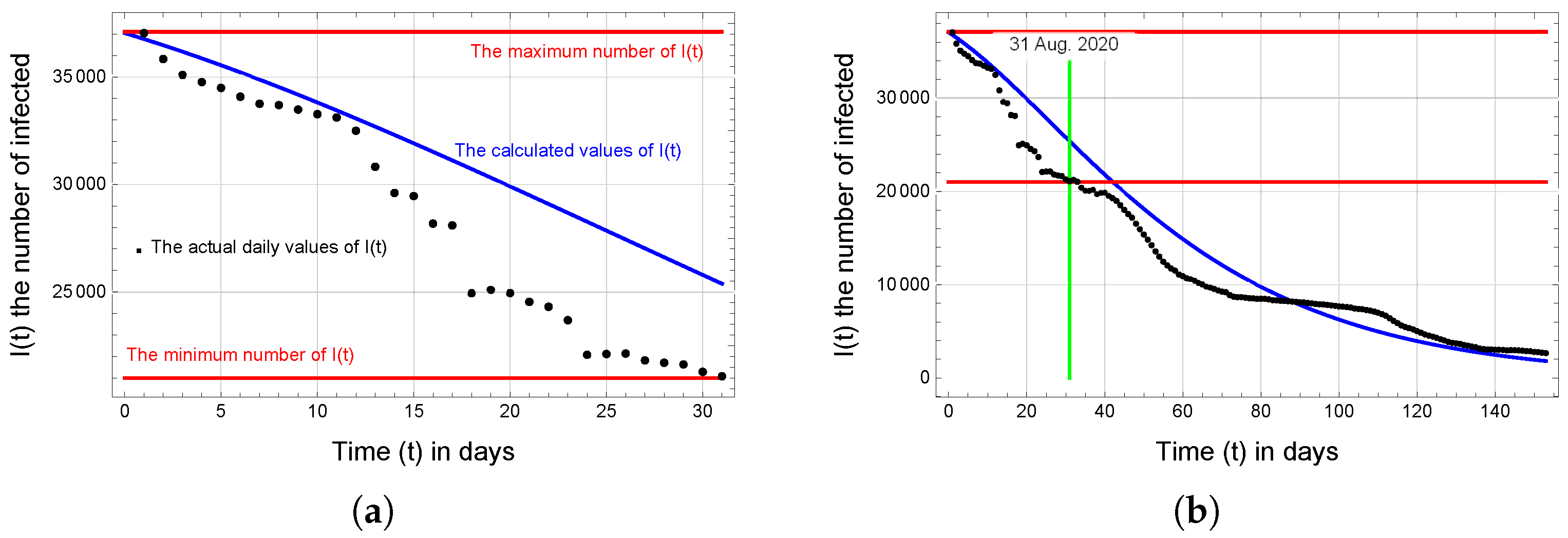Figure 7a illustrates that the number of active infected cases is decreasing and Figure 7b illustrates the behavior of the active infected cases along the overall period from the first of August to the end of December 2020, with the parameters calculated according to August data as in Table 1. It is shown that the number of active infected cases will continue in decreasing behaviors. The calculated data are close to the real data for the considered short time periods, and deviations in the calculated data appear for long periods. Our results are expected to be reached due to the change in the coefficients. The graphical behaviors, the decrease in $S\left(t\right)$ and the increase in $R\left(t\right)$ are conserved. Accordingly, the calculated results are reliable and can be used when designing for strategic planes.

4. Discussion

No one can deny the role of science and cognitive development in controlling many epidemic diseases that had devastating effects on humanity in different time periods. The mathematical models are considered one of the most important scientific developments in the field of epidemiological diseases, through which it is possible to develop scenarios to control the spread of diseases (such influenza) for the time periods. That enables medical scientists to introduce the appropriate treatments. The mathematical model of prey and predator represents the starting point for building epidemiological models. Moreover, strategies of dealing with epidemic diseases are inspired by methods of controlling predators and enhancing and supporting prey. This is done by studying rates of change in prey size. The prey sample under study is usually divided into groups:

The first group is predation and often represents the whole group at the start of the study. The second group is the one that is exposed to attempted predation. The third group is the one that is excluded from the second group, whether by defeating the attempted predation or by the actual predation. The problem lies in determining the style and method of movement between the three groups, which is called dynamical behaviors. Conventionally, most mathematical models in epidemiology works have believed that the incidence rate is (bilinear) proportional to the product of the numbers of susceptible and infective $\left(\beta SI\right)$. In this work, the accuracy of the calculated solutions rather than the behavior of the solution, are considered (decreasing of $S\left(t\right)$ and increasing of $R\left(t\right)$). To obtain accurate solutions, you must determine accurate values of the parameters of the model and solve the system with high accuracy and avoid the accumulation of errors. the SIR model is used over short time periods, so the accumulation of errors is controlled. Furthermore, the concept of upgrading the parameter values continuously is used. Recently, models which consider different dynamical behaviors, such as bifurcation or saddle-node bifurcations, have been introduced, and this will be our concern in subsequent separate work.

Thus, coping strategies can be divided into two styles:

The first style is to control the predator (disease), and that is done by eliminating it or limiting its efficacy (providing vaccinations). This method requires great capabilities and takes time.

The second style is to control the prey and train it to resist predation or avoid it in public. It is the fastest in application and has the least health side effects, the most obvious form of which is the application of social distancing. The side effects of using this style are its effects on the economy, education, and mental health, and the costs of its continuation.

Therefore, it was necessary to search for coping strategies that depend on the two styles, controlling the predatory specimen with the appropriate speed, as well as controlling the predator, and studying the methods that can be used. It is worth noting that the prey and predator model can be employed and used to study phenomena other than the spread of epidemics, such as studying dealing with information (rumors), studying drug prevalence rates (addiction), and studying the spread of some cultural characteristics (language and behaviors in general).

Many of the reported studies performed in different regions [3,21,22], and the references cited agree that numerical simulations are essential tools in dealing with any epidemic disease. Furthermore, raising the awareness of the community about the important impact of social distancing and population behavior in terms of contact and lockdown is an effective factor. As for spreading preventive culture (indirect control), it is recommended to do training of cadres on selecting, activating, developing mathematical models, selecting the appropriate mathematical models, feeding them with the correct data, developing appropriate strategies to deal with the available conditions, and updating them whenever circumstances permit. Community involvement through scientific studies is documented by field results.

5. Conclusions

Application of mathematical epidemic models should be restricted to short time scales. The SIR mathematical models, despite their simplicity, are still effective models that give acceptable results within limited time periods. Determination of the parameters of the models must be determined with more reliable techniques and should be updated continuously. Lockdown is the safest strategy despite its side effects in case of the absence of medical solutions. The introduced local forms of the SIR models are a remedy for the short time scale of the epidemic mathematical models and can be applied to other models effectively. Our calculated results are in high agreement with the recorded reports due to our local (short time) treatment. The acquired culture and the dissemination of health awareness help in raising morale and improving mood, which increases self-resistance. Great thanks to the authorities in the Kingdom of Saudi Arabia, the data that was calculated is consistent with all the data announced by the competent authorities during the considered periods.

In the future, we can use the implemented methodology of the present study to analyze different aspects of the research [25,26,27,28,29,30].