An Improved Self-Born Weighted Least Square Method for Cylindricity Error Evaluation

Abstract

In order to improve the stability of the evaluation results and the gross error resistance of the algorithm in view of the widespread gross errors in geometric error evaluation, an improved self-born weighted least square method (ISWLS) is proposed in this paper. First, the nonlinear cylindrical axial model is linearized to establish the error equation of the observed values. We use the conditional equations of the independent observations found as valid information to derive the weights of the observations. The weights of the observations are subjected to least-square iteration to calculate the error values and equation parameters. Meanwhile, the ordinal numbers of the independent sets of equations in the observed equations are updated several times. By updating the ordinal number information of the conditional equations, the influence of gross error data on the solution of the equations is minimized. Through a series of experiments, the algorithm is proved to have a strong resistance to gross differences, and operation time is shorter. According to the evaluation results of cylindricity error, the uncertainty of cylindricity error was calculated by the Guide to the expression of uncertainty in measurement method (GUM)and the Monte Carlo method (MCM). Experiments show that the uncertainty results of the MCM method can verify the results assessed by the GUM method, which proves that the results of the ISWLS method are effective and robust.

1. Introduction

Cylindricity error is an important basis for the acceptance of shaft parts. Accurate cylindricity error evaluation not only provides a reliable guarantee for improving the machining accuracy and assembly accuracy of parts but is also a prerequisite for stably improving production efficiency [1]. The spatial coordinate information of the measured point is measured, and the data are analyzed by an error evaluation algorithm to calculate the cylindricity error of the part [2]. The cylindricity error evaluation methods include the minimum zone cylinder method (MZC), least square cylinder method (LS), maximum inscribed cylinder method (MIC), and minimum circumscribed cylinder method (MCC). The minimum zone cylindrical method satisfies the minimum condition defined by the cylindricity error and is recognized as an arbitration method in case of inconsistent errors. Since it is an unconstrained nonlinear optimization problem, it cannot be solved directly by a computer. The least square method is widely used in the field of error evaluation by instruments such as the coordinate measuring machine (CMM), which has the advantages of mature theory, simple calculation, and stable evaluation results [3]. Since least square does not meet the minimum conditions defined by international standards, more in-depth research is required.

In recent years, many scholars have successfully applied the genetic algorithm [4], ant colony algorithm [5], artificial immune algorithm [6], artificial fish swarm algorithm [7], particle swarm algorithm [8], and other intelligent algorithms in geometric error assessment. In the field of geometric error evaluation, good results have been achieved. At the same time, more and more algorithms are proposed according to the characteristics of cylindricity error evaluation. He et al. [9] proposed a cylindricity error evaluation method based on the sequential quadratic programming algorithm, which uses coordinate simplification and the sequential quadratic programming algorithm to improve the accuracy of cylindricity error evaluation. Wu et al. [10] established an improved integrated learning particle swarm optimization algorithm applied to the cylindricity error evaluation problem to solve the local and globally optimal solutions of the cylindricity error evaluation results. Liu et al. [11] proposed a cylindricity error evaluation method based on incremental optimization. Li et al. [12] used the Hybrid Greedy Differential Evolution-Sine-Cosine Algorithm (HGSCADE) to solve optimization problems and evaluate cylindricity errors. Wang et al. [13] proposed a step-acceleration-based optimization algorithm to solve the efficiency problem of the crankshaft cylindricity error evaluation algorithm. The above methods for geometric error assessment have achieved good assessment accuracy, but the assessment methods are complicated, and further research and improvement are needed to improve the stability and robustness of the methods.

Based on the analysis of the observed data in production and experiments, statisticians observe that the probability of gross deviations is 1% to 10% of the total [14]. These gross errors seriously affect the error evaluation results. In the field of geodesy, to eliminate or attenuate the effect of gross errors on parameter estimation, Khaled et al. [15] proposed robust estimation to detect and eliminate gross errors at long distances. Guangfeng et al. [16] discussed the method of gross difference localization in detail: the “good” and “bad” points of gross difference are eliminated, but the “good” points are often eliminated as well. Jia et al. [17] studied the effectiveness of robust estimation in weakening and eliminating gross variances. The self-born weighted least square (SWLS) method is a robust estimation method with excellent robustness [18], which can effectively reduce the effect of gross differences, and the method is mainly applied in the field of mapping. It makes full use of the valid information provided by the conditional equations generated from independent observations to construct the weights of the observations, which can effectively eliminate or attenuate the effect of gross errors on parameter estimation. It is more effective than often other robust estimation methods [19]. At present, it has the advantages of simple theory and high accuracy of the assessment [20]. 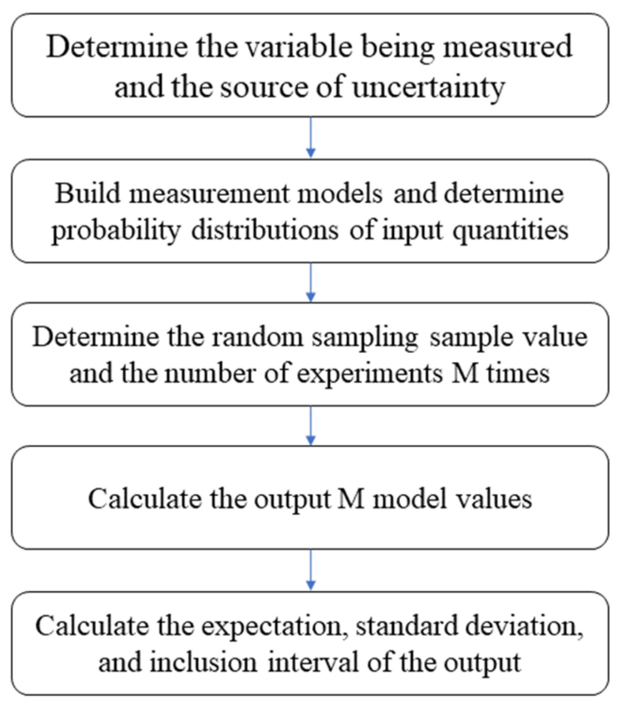It has a good effect in reducing or eliminating gross errors, etc., but its research and application in the field of geometric error assessment have not been reported [21]. The GUM and MCM methods are widely used in uncertainty assessment. When the calculated results of the GUM method can be verified by MCM, the uncertainty evaluation results have high reliability [8]. In this paper, we consider the introduction of the SWLS method into the field of geometric error assessment and improve the adaptability of the SWLS method by using cylindricity error evaluation as an example. By combining model initialization with the screening of independent groups, the technique is extended from linear model assessment to a broader range of nonlinear error assessment, improving the adaptability, accuracy, and operational speed of the method. Meanwhile, the GUM method and MCM method were also used to calculate the cylindricity error uncertainty in this paper, which proved the reliability of the error evaluation results.

2. Model of Least Square Solution of Cylindricity Error

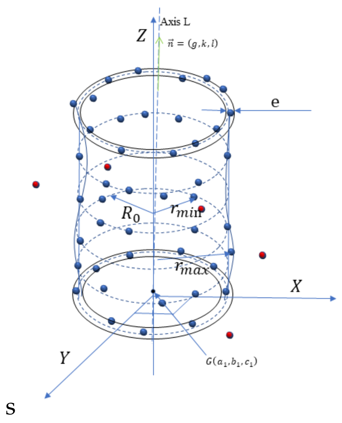
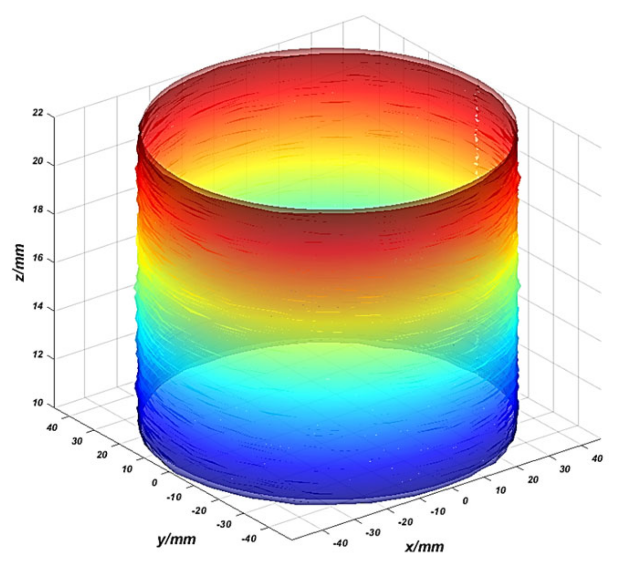
T Cylindricity error is the amount of deviation between the actual measured cylindrical surface and the ideal cylindrical surface, expressed as the difference between the radii of the two coaxial cylindrical surfaces. Assume that the measured coordinates in the right-angle coordinate system are $P_i\left(x_i,y_i,z_i\right)$, $i=1,2,3,\dots ,n$. The intersection point of the least square cylinder axis L and the cylinder interface is set as $G\left(a_1,b_1,c_1\right)$. The direction vector is set as $\overrightarrow{n}=\left(g,k,l\right)$. The equation of the axis $L$ is:

$$\frac{x-a_1}{g}=\frac{y-b_1}{k}=\frac{z-c_1}{l}$$

(1)

The axial L equation was simplified to obtain [13]:

$$\begin{gathered} \frac{x-a}{p}=\frac{y-b}{q}=z \\ p=\frac{g}{l},q=\frac{k}{l} \\ a=a_1-c_1\times \frac{g}{l}, b=b_1-c_1\times \frac{g}{l} \end{gathered}$$

(2)

The distance $d_i$. from each sampling point on the cylindrical surface to the axis is:

$$d_i=\sqrt{{\left[x_i-\left(p\times z_i+a\right)\right]}^2+{\left[y_i-\left(q\times z_i+b\right)\right]}^2}$$

(3)

The least square cylinder radius R is expressed as:

$$R=\frac{1}{n}{\displaystyle \sum }_{i=1}^n{d}_i$$

(4)

Then the objective function of the least square cylindrical method is [4]:

$$J=\min \left({\displaystyle \sum }_{i=1}^n{\left(d_i-R\right)}^2\right)$$

(5)

The cylindricity error is transformed into a search for the corresponding ideal cylindrical surface axis parameters $\left(a,b,p,q\right)$, which minimize the objective function J. From this, the least square cylinder axis L equation is obtained, and the maximum distance $R_{max}$ and the minimum distance $R_{min}$ from the actual measuring point to the axis are obtained. The diagram is shown in Figure 1. The corresponding cylindricity error:

$$e=R_{max}-R_{min}s$$

(6)

3. SWLS Solution for Cylindricity Error

3.1. Self-Born Weighted Least Square Robust Estimation Method

The SWLS method is a least square robust estimation method. It uses the observation correction number as the effective information provided by the conditional equation and constructs the weights with multiple estimates of the observation correction number. Compared with the ordinary least square method, the SWLS method uses the self-born weights of the observation value as the weights of the observation value, which effectively reduces the influence of gross errors.

SWLS assumes that the observation equation is of the linear form [18]:

$$\widehat{L}=B\widehat{x}+\left(d+B{X}^0\right)$$

(7)

The error equation is:

$$V=B\widehat{x}-l$$

(8)

$B$ is the coefficient matrix of the observation equation, $\widehat{L}$ is the estimated value of the observation value $L$, $V$ is the correct number of $L$, $\widehat{x}$ is the solution of the unknown, and $d$ is the constant term matrix of the observation equation. The unknown matrix $\widehat{X}=X^0+\widehat{x}$, where $X^0$ is the initial unknown value; $l=-\left(d+B{X}^0-L\right)$.

The solution $\widehat{x}$ of the unknown, the observed number of corrections $V,$ and the unit weighted variance valuation ${\widehat{\sigma }}^2$ can be obtained by using the least square method. $P$ is the weighted matrix; ${\dot{p}}_j$ is the diagonal element in the weighted matrix with an initial value of $1$.

$$\widehat{x}={\left(B^{T}PB\right)}^{-1}{B}^{T}Pl$$

(9)

$$V={\left(B^{T}PB\right)}^{-1}{B}^{T}Pl-l$$

(10)

$${\widehat{\sigma }}_0{}^2=\frac{V^{T}PV}{r}$$

(11)

The coefficient matrix $B$ in Equation (8) is transformed into $B_t$ and $B_r$, and $B_t$ is a $t\times t$ order full rank matrix; $n$. is the number of observations, and t is the number of parameters to be requested. Meanwhile, $V$ and $l$ are matrix transformed to obtain $V_t$ and $l_t$:

$$V_t=B_t\widehat{x}-l_t$$

(12)

$$V_r=B_r\widehat{x}-l_r$$

(13)

According to formulas (12) and (13), we can obtain:

$$\widehat{x}=B_t^{-1}\left(V_t+l_t\right)$$

(14)

$$V_r=B_{rt}{V}_t-W_{rt}$$

(15)

In the formula, $B_{rt}=B_r{B}_t^{-1}$, $W_{rt}=-\left(B_r{B}_t^{-1}{l}_t-l_r\right)$. Both $B_t$ and $B_r$ are not unique and are primarily chosen by independent groups.

Since the absolute value of the accidental error has a finite value, $\eta {\widehat{\sigma }}_0$ is used to limit the unit weighted error to a certain estimation range, and $\eta$ is the value range coefficient (take 3 according to the simulation experiment). From Equations (12) and (13), the m groups of true error estimates $V^{\left(1\right)}$ that satisfy Equation (16) are obtained, $V^{\left(1\right)}, V^{\left(2\right)}$, …, $V^{\left(m\right)}$ are:

$$V^{\left(i\right)}={\left[v_1^{\left(i\right)} v_2^{\left(i\right)} \dots v_n^{\left(i\right)}\right]}^T, i=1,2, \dots ,m$$

(16)

$$\left|v_j^{\left(i\right)}\right|\le \frac{\eta {\widehat{\sigma }}_0}{\sqrt{p_j}} i=1,2,\dots ,m; j=1,2,\dots ,\mathrm{n}$$

(17)

In the formula, when $v_j^{\left(i\right)}\in V_t$, $-\frac{\eta {\widehat{\sigma }}_0}{\sqrt{p_j}}$ is the initial value of $v_j^{\left(i\right)}$, $\frac{\eta {\widehat{\sigma }}_0}{\sqrt{p_j}}$ is the final value of $v_j^{\left(i\right)}$, and $\frac{\eta {\widehat{\sigma }}_0}{\theta \sqrt{p_j}}$ is the step size when $v_j^{\left(i\right)}\in V_r$, $v_j^{\left(i\right)}$ is determined by Equation (15) [18]; $p_j$ is the diagonal element of the weighted matrix generated by the previous iteration.

The self-born variance is the variance of the observed value calculated from m estimates of the true error of the same observation value. The reproduction weights are the weights of the observation value calculated from the reproduction variance of the observation value. Then, the self-born variance ${\dot{\sigma }}_j$, self-born variance ${\overline{\sigma }}_0$, and self-born weights ${\dot{p}}_j$ generated from different observations are calculated as follows:

$${\dot{\sigma }}_j^2=\frac{1}{m}{\displaystyle \sum }_{i=1}^m{\left(v_j^{\left(i\right)}\right)}^2 j=1,2,\dots , n$$

(18)

$${\overline{\sigma }}_0^2=\frac{1}{n}{\displaystyle \sum }_{j=1}^n{\dot{\sigma }}_j^2$$

(19)

$${\dot{p}}_j=\frac{{\overline{\sigma }}_0^2}{{\dot{\sigma }}_j^2} j=1,2, \dots ,n$$

(20)

The calculated self-born weight ${\dot{p}}_j$ is taken into the weights of the observation value, and the correction number $V$ of the observation value and the error ${\widehat{\sigma }}_0$ in the unit weights are calculated by the least square method. The iteration terminates when the adjacent observation correction number iteration difference is less than the limit.

3.2. Insufficiency of Self-Born Weighted Least Square Method

SWLS is mainly applied in linear regression, and it uses analytical calculations to solve the error equation. It has not been studied for nonlinear problems and needs to be further optimized and explored. SWLS has certain requirements for the choice of independent groups in the observations and uses the number of observation corrections as valid information supplied by the conditional equation. It is necessary to artificially modify the selection of independent groups in various application settings. The outcomes will exhibit significant variances when the independent group was improperly chosen and includes serious flaws. In geometric error evaluation (e.g., CMM evaluation of geometric errors), producers need measurement methods that are more efficient, accurate and adaptable. The adjustment of the independent group will lead to an increase in production costs as well as a decrease in adaptability and accuracy, so the SWLS method is needed for further improvement.

3.3. Improved self-Born weighted Least Square Method

In response to the above shortcomings, this paper improves the SWLS method to increase the effectiveness of the method. The improved method is called ISWLS. In this paper, we take the calculation of cylindricity error as an example and apply the SWLS method to linearize the nonlinear model to calculate the cylindrical axis equation and cylindricity error. Additionally, an automatic selection step of the independent equation sets is implemented to lessen the impact of the choice of independent equation sets on the outcomes. It eliminates the manual filtering step of the independent group equations and makes the calculation simplified. The calculation steps are as follows:

3.3.1. Model Initialization

To apply the SWLS method to a nonlinear problem, the nonlinear model must first be transformed into a linear model. The model equations are assumed to be:

$$Z=F\left(X\right)$$

(21)

In order to linearize the equation, a sufficient approximation $X^0$ of $\tilde{X}$ is taken [19]:

$${\tilde{X}}_i=X_i^0+\tilde{x} , \left(i=1,2,\dots ,n\right)$$

(22)

$\mathrm{Because} \tilde{x}$ is a tiny quantity, the Taylor formula can be used to omit the quadratic and more than quadratic terms [22], and then the functional equation is:

$$\begin{gathered} Z=F\left(X_1^0,X_2^0, \dots ,X_n^0\right)+\left(\frac{\partial F}{\partial X_0}\right)\tilde{x}+\left(\frac{\partial F}{\partial X_1}\right)\tilde{x} \\ +\left(\frac{\partial F}{\partial X_2}\right)\tilde{x}+\dots +\left(\frac{\partial F}{\partial X_n}\right)\tilde{x}+\Delta \left(\mathrm{higher} \mathrm{order} \mathrm{terms}\right) \end{gathered}$$

(23)

Bringing Equations (3)–(5) into Equation (23), it is expressed in matrix form as:

$$J=\left[b_1 b_2 b_3 b_4 b_5\right]\left(\begin{array}{c}\delta \widehat{a}\\ \delta \widehat{b}\\ \delta \widehat{p}\\ \delta \widehat{q}\\ \delta \widehat{R}\end{array}\right)-D_i$$

(24)

Equation parameters:

$$\begin{gathered} {\epsilon }_1=a-x_i+p\times z_i, {\epsilon }_2=b-y_i+q\times z_i \\ {b}_1=\frac{{\epsilon }_1}{\sqrt{{\epsilon }_1{}^2+{\epsilon }_2{}^2}}, b_2=\frac{{\epsilon }_2}{\sqrt{{\epsilon }_1{}^2+{\epsilon }_2{}^2}} \\ {b}_3=\frac{{\epsilon }_1\times z_i}{\sqrt{{\epsilon }_1{}^2+{\epsilon }_2{}^2}}, b_4=\frac{{\epsilon }_2\times z_i}{\sqrt{{\epsilon }_1{}^2+{\epsilon }_2{}^2}} \\ {b}_5=-1; D_i={(R-\sqrt{{\epsilon }_1{}^2+{\epsilon }_2{}^2})}^2 \\ \delta \widehat{a}=a-a_0, \delta \widehat{b}=b-b_0, \delta \widehat{p}=p-p_0, \delta \widehat{q}=q-q_0 \end{gathered}$$

$\mathrm{The} \mathrm{initialization} \mathrm{parameters} \mathrm{are} a_0, b_0, p_0, q_0, \delta \widehat{R}$, and they are determined by the coordinates of the measurement cylinder center position.

3.3.2. Calculation of the Self-Born Weights Function

Equation (24) is divided into t levels according to the number of unknowns, and the first set of equations in each level is selected and combined into a linearly independent combination of error equations. The error equation is expressed as:

$$V_t=B_t\widehat{x}-l_t$$

(25)

$$V_r=B_r\widehat{x}-l_r$$

(26)

Equation (25) is the set of independent equations, and Equation (26) is the set of conditional equations before iteration. Then, according to Equation (9) to Equation (11), the solution $\widehat{x}$ of the unknown, the number of observed corrections $V,$ and the unit weighted variance valuation ${\widehat{\sigma }}^2$ can be obtained.

3.3.3. Self-Born Weight Iteration and Parameter Calculation

The self-born weights that were calculated were brought into Equation (8) to calculate the number of corrections and unit weight errors of the observations. The new self-born weights are calculated from Equations (18)–(20). The newly calculated self-born weights are brought into Equation (8) to calculate the new number of corrections V and the unit weight errors. The iteration condition is set to correct the number V before and after the difference of the iteration value is less than $\Delta$. The gross error weights far from the column surface are reduced. The axial parameter and cylindricity error are output.

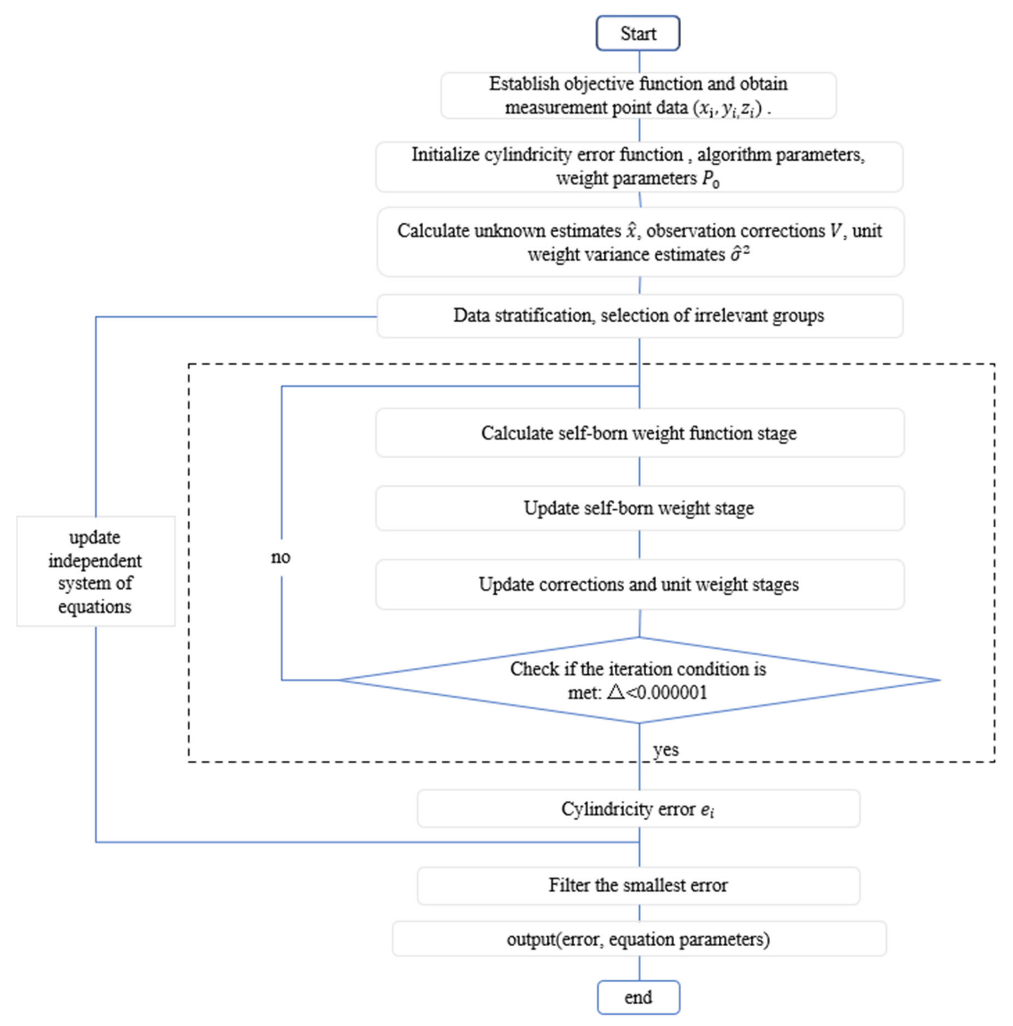
3.3.4. Updating of the Independent Equations

The independent set of equations is Equation (25), and the initial order of the independent set of equations has been obtained from step (2). The number of updates of the independent set of equations is set enough (the number of updates is generally set to the number of samples per level). Step (2) and step (3) are repeated. The set of data with the smallest error is selected. The errors and equation parameters are output. We set enough random sampling times and repeat steps (2) to (3) until a set of data with the smallest error was selected. The number of iterations is determined by the amount of data in each layer. The error and equation parameters are output. The algorithm flow chart is shown in Figure 2.

4. Cylindricity Error Uncertainty Evaluation

4.1. GUM Assessment Method

Currently, the GUM method is the most commonly used method in uncertainty evaluation. According to the GUM method, the uncertainty propagation rate model is determined, and the uncertainty source of each parameter is determined at the same time. The composite standard uncertainty and expanded uncertainty of the cylindricity error uncertainty evaluation are calculated. The sources of uncertainty are analyzed as follows:

(1) Repeat the measurement at a single point 10 times, and the introduced uncertainty component $u_1$ is calculated according to the Bessel formula [3]:

$$u_1=\sqrt{\frac{{{\displaystyle \sum }}_{i=1}^n{\left(x_i-\overline{x}\right)}^2}{n-1}}$$

(27)

(2) The uncertainty component caused by the indicated value error can be derived from the measurement experience of the instrument. The maximum allowable indication error $\sigma$ of the CMM is $0.5 \mathsf{\mu }\mathrm{m}$. The coverage factor k is $\sqrt{3}$. The indication error is expressed as $u_2$ [3]:

$$u_2=\frac{\sigma }{k}$$

(28)

(3) During the test, the room temperature is kept constant at 20 degrees Celsius, so the uncertainty $u_3$ caused by the temperature is approximately 0$\mathsf{\mu }\mathrm{m}$ [3].

(4) In practical measurements, the uncertainty component $u_4$ is approximated as 0$\mathsf{\mu }\mathrm{m}$ due to the deformation caused by the measuring force [3].

Then the single-point uncertainty $u_0$ is calculated as [3]:

$$u_0=\sqrt{u_1^2+u_2^2+u_3^2+u_4^2}$$

(29)

According to the actual situation, the conditions of a single measurement tend to be the same, and the single-point uncertainty is:

$$u_{xmax}=u_{ymax}=u_{zmax}=u_{xmin}=u_{ymin}=u_{zmin}=u_0$$

(30)

The key to calculating the uncertainty is to find the uncertainty u and ρ of each parameter as the correlation coefficient of each parameter. Uncertainties of $a,b,p,q$ are obtained from actual data. Suppose the vector $D={\left[a,b,p,q\right]}^T$, then

$$cov\left(D\right)=\left[\begin{array}{cccc}var\left(a\right)& cov\left(a,b\right)& cov\left(a,p\right)& cov\left(a,q\right)\\ cov\left(b,a\right)& var\left(b\right)& cov\left(b,p\right)& cov\left(b,q\right)\\ cov\left(p,a\right)& cov\left(q,a\right)& cov\left(p,b\right)& cov\left(q,b\right)\\ var\left(p\right)& cov\left(q,p\right)& cov\left(p,q\right)& var\left(q\right)\end{array}\right]$$

The correlation coefficient can be calculated according to Equation (31) as follows:

$${\rho }_{ab}=\frac{u_{ab}}{u_a{u}_b}$$

(31)

Finally, the synthetic standard uncertainty $u_{\delta }$ is calculated according to the GUM method:

$$\begin{gathered} u_{\delta }^2={\left(\frac{\partial f}{\partial x_{max}}{u}_{xmax}\right)}^2+{\left(\frac{\partial f}{\partial y_{max}}{u}_{ymax}\right)}^2+{\left(\frac{\partial f}{\partial z_{max}}{u}_{zmax}\right)}^2 \\ +{\left(\frac{\partial f}{\partial x_{min}}{u}_{xmin}\right)}^2+{\left(\frac{\partial f}{\partial y_{min}}{u}_{ymin}\right)}^2+{\left(\frac{\partial f}{\partial z_{min}}{u}_{zmin}\right)}^2 \\ +{\left(\frac{\partial f}{\partial p}{u}_p\right)}^2+{\left(\frac{\partial f}{\partial q}{u}_q\right)}^2+{\left(\frac{\partial f}{\partial a}{u}_a\right)}^2+{\left(\frac{\partial f}{\partial b}{u}_b\right)}^2 \\ +2\frac{\partial f}{\partial a}\frac{\partial f}{\partial b}{\rho }_{ab}{u}_{ab}+2\frac{\partial f}{\partial a}\frac{\partial f}{\partial p}{\rho }_{ap}{u}_{ap}+2\frac{\partial f}{\partial a}\frac{\partial f}{\partial q}{\rho }_{aq}{u}_{aq} \\ +2\frac{\partial f}{\partial b}\frac{\partial f}{\partial p}{\rho }_{bp}{u}_{bp}+2\frac{\partial f}{\partial b}\frac{\partial f}{\partial q}{\rho }_{bq}{u}_{bq}+2\frac{\partial f}{\partial p}\frac{\partial f}{\partial q}{\rho }_{pq}{u}_{pq} \end{gathered}$$

(32)

4.2. MCM Assessment Method

The Monte Carlo sampling method evaluation (MCM) can be used as a supplementary verification method to GUM or as a stand-alone method for uncertainty evaluation. The MCM method is mainly divided into three steps: input, propagation, and output. The evaluation steps are shown in Figure 3.

4.3. Validation of GUM Method Results by MCM Method

In order to evaluate the applicability of the GUM experimental results, the results of the GUM method need to be validated using the MCM method. The inclusion interval $y\pm U_p$ of the inclusion probability p (taken as $95\%$ in this paper) of the output quantity is calculated using the GUM method. The standard uncertainty $u\left(y\right)$ of the MCM output quantity and the endpoint values $y_{low}$ and $y_{high}$ of the shortest inclusion interval are calculated. Finally, the absolute value deviation of the respective endpoints is found by Equations (17) and (18). When the absolute deviations $d_{low}$ and $d_{high}$ of the respective endpoints of the two included intervals are less than or equal to the numerical tolerance δ of the uncertainty, the GUM can be verified, indicating that the GUM assessment results are consistent with the actual situation [3].

5. Experimental Verification and Literature Verification

5.1. Experimental Verification

Experimentally, a part of the shaft segment was selected for measurement with a nominal diameter of $\Phi =92 \mathrm{mm}$. The measuring equipment was the German Zeiss CMM PRISMO 9/13/7 ultra-type three-coordinate measuring machine to measure the outer ring of the shaft. According to the ISO 12180-2:2011 standard cylindricity measurement guidelines, various point assignment strategies can be employed, including measurement methods such as roundness (circumference) profiles, bus bars, bird cages, spirals, and random points [22,23]. The circle profile method was selected in the experiment, 5 sections were measured, and 48 points were measured at equal angular intervals on each section. The experiment is shown in Figure 4.

5.1.1. Evaluation of Experimental Data

The least square objective function was constructed from the sampled point data. Then the least square (LS), self-born weighted least square (SWLS), improved self-born weighted least square (ISWLS), standard particle swarm algorithm (standard PSO), and standard genetic algorithm (standard GA) were used to calculate the cylindricity error, respectively. The selection of the irrelevance group of the SWLS method followed the actual situation, and the 1st, 57th, 112th, 167th, and 222nd error equations were selected as the 5 error equations that make up the maximum linear independence group. The number of updates of the independent system of equations was 30 when the experiment uses the ISWLS method. The population size of the genetic algorithm was 200, the number of evolutions was 2000, and the crossover probability and mutation probability were 0.7 and 0.2. The particle swarm optimization population size was 500, the number of evolutions was 1000, and the learning factors were c1 = c2 = 2. The results of the first group of measurement data processing are shown in

Table 1. The first set of data evaluates the results.

Evaluation Method	Axis Parameters
	$\mathbf{a} \left[\mathit{m}\mathit{m}\right]$	$\mathbf{b} \left[\mathit{m}\mathit{m}\right]$	$\mathbf{p} \left[\mathit{m}\mathit{m}\right]$	$\mathbf{q} \left[\mathit{m}\mathit{m}\right]$
LS	0.0004	0.0000	−0.0009	−0.0007
SWLS	−0.0087	−0.0010	0.0004	0.0000
ISWLS	0.0267	0.0275	−0.0010	−0.0010
PSO	0.0003	0.0010	0.0142	0.0943
GA	−0.0013	−0.0008	0.0256	0.0141
Evaluation Method	Cylindricity Error $\left[mm\right]$		Running Time $\left[s\right]$
LS	0.1955		0.074023
SWLS	0.1346		0.177704
ISWLS	0.1336		0.082950
PSO	0.1415		7.467153
GA	0.1514		15.34568

. At the same time, the fitting result of the ISWLS method is shown in Figure 5.

In Table 1, the cylindricity axis parameters, cylindricity error value and calculation time were calculated, and it can be seen that the axis positions calculated by the five methods are slightly different. The cylindricity error value of the LS method was 0.1955 mm, which was significantly larger than the error of other algorithms. The standard PSO method and the standard GA method were global optimization algorithms with cylindricity error results of 0.1415 mm and 0.1514 mm, respectively, and the computing time was more than 7 s. The results were more accurate than those of the LS method, but the computation time was longer. The cylindricity error results of the ISWLS method and SWLS method were 0.1346 mm and 0.1336 mm, respectively. Their operation time were 0.0977 s and 0.08295 s, respectively. They both had higher accuracy compared to the LS method and shorter operation time than the standard PSO and standard GA methods. Since the operation time of the ISWLS method did not include the selection time of the independent set of equations, and the influence of gross errors on the selection of the independent set of equations was guaranteed to be excluded in each operation, the algorithm is generally better than the SWLS method.

Under the same conditions, the same sampling method was used to measure the same measurement object 10 times, and the error data were obtained by using the four methods of processing in Section 5.1.1, as shown in Figure 6.

As can be seen from Figure 6, the cylindricity error values calculated by the ISWLS method were consistent with those of the SWLS method, LS method, standard PSO method, and standard GA method in the evaluation of 10 measurement results, which indicated the effectiveness of the ISWLS method. The value of cylindricity error found by the LS method is larger than the value of other algorithms. The standard PSO method and the standard GA method were global optimization algorithms, and the trend of the evaluation error values for the 10 sets of measurement data was the same as that of the LS method, but the evaluation error values were significantly lower. When the SWLS method was used for cylindricity error assessment, the stability of the assessment results was poor because of the different effects of the independent groups in the selection on the assessment results, and some of the cylindricity error values were large compared with the results of the standard PSO method and the standard GA method, which was similar to the LS method. The evaluation error values of each group of the ISWLS method were smaller than those of the SWLS method and LS method. The evaluation results of the ISWLS method were similar to those of the standard PSO method and standard GA method, and the results were stable and have higher accuracy.

5.1.2. Error Evaluation after Inserting Gross Error Points

Considering the influence of gross differences on the error assessment, a numerical experiment of inserting gross differences was designed. According to the existing measurement data, the column surface points of one measurement were selected, and three gross error points were inserted randomly in the 1st, 2nd, and 3rd layer measurement sections to observe the change of the axis position. The insertion of the gross difference data is shown in

Table 2. Insertion point data.

No.	$\mathbf{X} \left[\mathit{m}\mathit{m}\right]$	$\mathbf{Y} \left[\mathit{m}\mathit{m}\right]$	$\mathbf{Z} \left[\mathit{m}\mathit{m}\right]$
1	46.28403	10.00008	22
2	34.63978	12.22836	19
3	−55.36314	9.22029	16

. The ISWLS method was used to calculate the axial parameters and cylindricity error values, and the results are shown in

Table 3. Evaluation results of ISWLS method when inserting gross error points.

Insert Gross Point	Axis Parameters
	$\mathbf{a} \left[\mathit{m}\mathit{m}\right]$	$\mathbf{b} \left[\mathit{m}\mathit{m}\right]$	$\mathbf{p} \left[\mathit{m}\mathit{m}\right]$	$\mathbf{q} \left[\mathit{m}\mathit{m}\right]$
0	−0.0087	−0.0010	0.0004	0.0000
1	−0.0467	−0.0092	0.0033	0.0007
2	0.0786	0.0356	−0.0090	−0.0038
3	−0.0027	0.0488	−0.0090	−0.0038
Insert Gross Point	Cylinder Radius r $\left[mm\right]$		Cylindricity Error $\left[s\right]$
0	46.2909		0.1336
1	46.2953		0.1475
2	46.2966		0.1875
3	46.2998		0.2038

.

In order to reflect the influence of the gross difference value on the error results before and after the iteration of the ISWLS method, the true error value $v^{\left(i\right)}$ of Equation (16) in the ISWLS method was selected as the variable, and the true error values $v^{\left(i\right)},\left(i=1,\dots ,240\right)$ of 240 points on the column before the iteration were compared with the calculated results after the iteration, as shown in Figure 7.

According to Figure 7a, the true error value $v^{\left(i\right)}$ did not change much before and after the iteration when the gross error point was not inserted, and the result was more stable. As shown in Figure 7b, the true error value $v^{\left(i\right)}$ at the beginning of the iteration was 0.95 mm larger than that at the rest of the points after inserting a gross point, and the deviation of the true error value $v^{\left(i\right)}$ at the gross point was reduced to normal after the end of the iteration. As shown in Figure 7c, after the insertion of 2 gross points, the maximum true error value $v^{\left(i\right)}$ at the 2 gross points inserted at the beginning of the iteration was 9.5 mm compared to the remaining points, and the true error values $v^{\left(i\right)}$ at the gross points can converge to the normal value after the end of the iteration. According to Figure 7d, after the insertion of three gross points, the maximum true error value $v^{\left(i\right)}$ at the three gross points inserted at the beginning of the iteration was 9.8 mm larger than the deviation of the remaining points, and the maximum deviation of the true error value $v^{\left(i\right)}$ at the gross points returned to 0.2 mm after the end of the iteration. It can be seen that the true error values of cylindricity at each point are larger under the influence of inserting gross error points. The true error parameter values of the gross difference part tended to be smooth after iteration. It reflected that the ISWLS method was very effective in reducing the influence of gross errors.

According to Table 3, it can be seen that the radius of the cylindrical fit of the ISWLS method was 46.2953 mm for the insertion of one gross point. The radius of the cylindrical fit was 46.2966 mm for the insertion of two gross points. The radius of the cylindrical fit was 46.2998 mm when three gross points were inserted. Compared to when gross error point was not inserted, the cylindrical radius changed within 0.01 mm, and the algorithm had better resistance to gross error. Cylindricity error was 0.1336 mm when gross error point was not inserted. Cylindricity error was 0.1475 mm when one gross error point was inserted. The cylindricity error was 0.1875 mm when two gross error points were inserted. The cylindricity error was 0.2038 mm when three gross error points were inserted. With the increase of inserting gross error points, the cylindricity error changed within 0.08 mm, and the data change was small. This shows that the algorithm can reduce the influence of gross error on the evaluation results, had a certain resistance to gross error, and had good robustness.

5.1.3. Comparison and Evaluation of Algorithms after Inserting Gross Error Points

The ISWLS algorithm differed from other algorithms in terms of its ability to resist gross differences. The standard PSO, standard GA, SWLS, and ISWLS methods were used to compare the error ratings according to the number of insertion gross error point. The comparison results are shown in

Table 4. Error evaluation results of different algorithms when inserting gross error points (mm).

Evaluation Method	1 Gross Error Point [mm]	2 Gross Error Points [mm]	3 Gross Error Points [mm]
LS	1.1775	10.6446	19.0610
SWLS	0.1681	0.2130	0.2911
ISWLS	0.1475	0.1875	0.2038
PSO	1.0698	10.2447	10.8566
GA	1.4444	9.2046	9.4694

and Figure 8.

As can be seen from Table 4, when one gross error point was inserted, the cylindricity error of the ISWLS method was 0.1475 mm, the cylindricity error of the SWLS method was 0.1681 mm, and the cylindricity errors of the standard PSO method, standard GA method, and LS method were 1.0698 mm, 1.4444 mm, and 1.1775 mm respectively, which showed that the five algorithms were gradually affected by gross errors. ISWLS had a better ability to resist gross error than SWLS. SWLS had a better ability to resist gross error than other algorithms. When two gross error points were inserted, the cylindricity error of the ISWLS method was 0.1875 mm, and the cylindricity error of the SWLS method was 0.2130 mm. The cylindricity errors of the standard PSO method, standard GA method, and LS method were 10.2447 mm, 9.2046 mm, and 10.6446 mm, respectively. When the number of gross error points increased, the five algorithms were affected by the number of gross error increases. As the number of gross error points increased, ISWLS outperformed SWLS, PSO, GA, and LS in resisting gross errors, and their ability to resist gross errors gradually declined. When three gross error points were inserted, the cylindricity error of the ISWLS method was 0.2038 mm, that of the SWLS method was 0.2911 mm, and that of the standard PSO method, standard GA method, and LS method were 10.8566 mm, 9.4694 mm and 19.0610 mm, respectively. The ISWLS method had less error change than the SWLS method, and its ability to resist gross error was significantly better than that of standard PSO and standard GA methods, while the cylindricity error of the LS method increased significantly with the increase of gross error points, and the ability to resist gross error declined significantly.

As can be seen from Figure 8, with the increase in inserting gross error points, the LS method was most affected by the gross error points, and the cylindricity error value increased gradually. The standard PSO and standard GA methods had a significant decrease in the error elevation of the cylindricity error value after the insertion of the 2nd error point due to the reason of the gross error point location and the advantage of the algorithm. The ISWLS method and the SWLS method had a certain resistance to gross errors. Compared with other algorithms, the cylindricity error assessment results did not increase significantly after inserting gross error points, the changes were relatively flat, and the ISWLS method was more resistant to gross errors than the SWLS method.

5.2. Literature Verification

To verify the method proposed in this paper, data samples of the literature [4] were used in this paper to evaluate the cylindricity error. The 24 data points are shown in

Table 5. Coordinates of points in reference [4]. Reprinted with permission from Ref. [4]. 2004, Wen, X.L.; Song, A.

No.	$\mathbf{X} \left[\mathit{m}\mathit{m}\right]$	$\mathbf{Y} \left[\mathit{m}\mathit{m}\right]$	$\mathbf{Z} \left[\mathit{m}\mathit{m}\right]$	No.	$\mathbf{X} \left[\mathit{m}\mathit{m}\right]$	$\mathbf{Y} \left[\mathit{m}\mathit{m}\right]$	$\mathbf{Z} \left[\mathit{m}\mathit{m}\right]$
1	11.0943	0.4522	65.2328	13	10.815	0.5918	85.2307
2	5.094	10.845	65.0765	14	4.8148	10.9846	85.074
3	−6.9063	10.8439	65.0089	15	−7.1855	10.9835	85.0641
4	−12.9065	0.4498	65.0897	16	−13.185	0.5894	84.8952
5	−6.9063	−9.9429	65.054	17	−7.1855	−9.8033	85.0516
6	5.094	−9.9418	65.2216	18	4.8149	−9.8022	85.2171
7	10.9546	0.522	75.2316	19	10.6754	0.6616	95.2291
8	4.9544	10.9148	75.0752	20	4.6752	11.0544	95.0728
9	−7.0459	10.9137	75.077	21	−7.3253	11.0533	94.9077
10	−13.0461	0.5196	74.8964	22	−13.3254	0.6592	95.094
11	−7.0459	−9.8731	75.0528	23	−7.3252	−9.7335	95.0504
12	4.95447	−9.872	75.2204	24	4.6752	−9.7323	95.2179

. Reference [4] used the genetic algorithm to evaluate three cylindricity error model methods, including the minimum area method, the minimum circumscribed cylinder method, and the maximum inscribed cylinder method. The error evaluation results based on the MZC, MCC, and MIC methods in the literature [4] are shown in

Table 6. The data evaluation results in the literature [4]. Reprinted with permission from Ref. [4]. 2004, Wen, X.L.; Song, A.

Evaluation Method	Axis Parameters				Cylindricity Error $\left[\mathit{m}\mathit{m}\right]$
	$\mathbf{a} \left[\mathit{m}\mathit{m}\right]$	$\mathbf{b} \left[\mathit{m}\mathit{m}\right]$	$\mathbf{p} \left[\mathit{m}\mathit{m}\right]$	$\mathbf{q} \left[\mathit{m}\mathit{m}\right]$
MZC	0.0024	−0.0040	−0.0140	0.0070	0.00279
MCC	0.0025	−0.0042	−0.0140	0.0070	0.00282
MIC	0.0037	−0.0039	−0.0140	0.0070	0.00279

. The ISWLS, LS, PSO, and GA methods were used to evaluate the error of the least square cylinder method for the sampling point data, and the setting parameters were consistent with the above. The error evaluation results are shown in

Table 7. ISWLS method data evaluation results.

Evaluation Method	Axis Parameters
	$\mathbf{a} \left[\mathit{m}\mathit{m}\right]$	$\mathbf{b} \left[\mathit{m}\mathit{m}\right]$	$\mathbf{p} \left[\mathit{m}\mathit{m}\right]$	$\mathbf{q} \left[\mathit{m}\mathit{m}\right]$
LS	−0.0140	0.0070	0.0036	−0.0046
PSO	0.0024	−0.0250	−0.0139	0.0069
GA	0.0045	−0.0068	−0.0140	0.0070
ISWLS	0.0037	−0.0034	−0.0140	0.0070
Evaluation Method	Cylindricity Error $\left[mm\right]$		Running Time $\left[s\right]$
LS	0.00288		0.034277
PSO	0.00286		6.508752
GA	0.00279		12.568197
ISWLS	0.002788		0.041420

.

Comparing Table 6 and Table 7, it can be seen that the method proposed in this paper was consistent with the results obtained in the literature, and the evaluation error was smaller.

5.3. Cylindricity Error Uncertainty Experiment

According to the first group of cylindricity error evaluation data in Table 1, the cylindricity error uncertainty was calculated by the ISWLS method. The combined standard uncertainty of the output was calculated, and the inclusion interval of the 95% inclusion probability was obtained for the interval factor k = 1.96. The data are shown in

Table 8. GUM method evaluation results of the first set of data.

Parameter	Value $\left[\mathit{\mu }\mathit{m}\right]$	Name	Value $\left[\mathit{\mu }\mathit{m}\right]$
$u_1$	0.0052	$u_a$	0.3274
$u_2$	1.556	$u_b$	0.3274
$u_3$	0	$u_p$	0.0012
$u_4$	0	$u_q$	0.0012
$u_0$	1.560	$u_{\delta }$	2.2216
Parameter	Value $\left[mm\right]$
best estimate	0.1338
95% probability inclusion interval	[0.1294, 0.1381]

.

The MCM method, as a supplementary method to the GUM method, can perform an uncertainty assessment of cylindricity error. The results can be compared with the GUM method. The results are shown in

Table 9. MCM method evaluation results of the first set of data.

Parameter	$\mathbf{Value} \left[\mathit{m}\mathit{m}\right]$
best estimate	0.1338
95% probability inclusion interval	[0.1294, 0.1381]
Project	$d_{low}$	$d_{high}$	MCM verifies GUM results (δ ≤ 0.0005)
MCM Verification GUM	0.0002	0.0001	Yes

and Figure 9.

5.4. Analysis of Results

The ISWLS was compared with the standard PSO, standard GA, and LS methods through experiments and literature validation. It was proved that ISWLS satisfies the definition. A more accurate cylindricity error evaluation result and a shorter running time were obtained. By inserting gross errors, it was verified that the ISWLS method is more resistant to gross errors than other algorithms, with more stable results and better robustness. The uncertainty of the cylindricity error was evaluated by the GUM method and the MCM method. The result of the GUM method was 0.002222 mm and the result of the MCM method was 0.002349 mm. The absolute deviations of $d_{low}$ and $d_{high}$ for each endpoint of the two included intervals were 0.0002 and 0.0001, which was less than the uncertainty value tolerance of 0.0005. The uncertainty results of the MCM method can verify the results of the GUM method, which proved the validity of the results and the robustness of the ISWLS method.

6. Conclusions

Since there are cases of gross errors in cylindricity error evaluation, this paper proposes the ISWLS method to evaluate the cylindricity error. The algorithm was compared with the standard PSO, standard GA, and LS methods for error assessment. The ability of the algorithm to resist gross errors was verified by inserting gross error points, and the correctness of the algorithm was verified using literature data. The experimental results show that:

(1) The method in this paper differs from SWLS and conventional global optimization algorithms in that it does not require setting parameters such as independent group order, population size, and crossover variation, and the operation steps are simple. As a result, the algorithm is relatively simple.

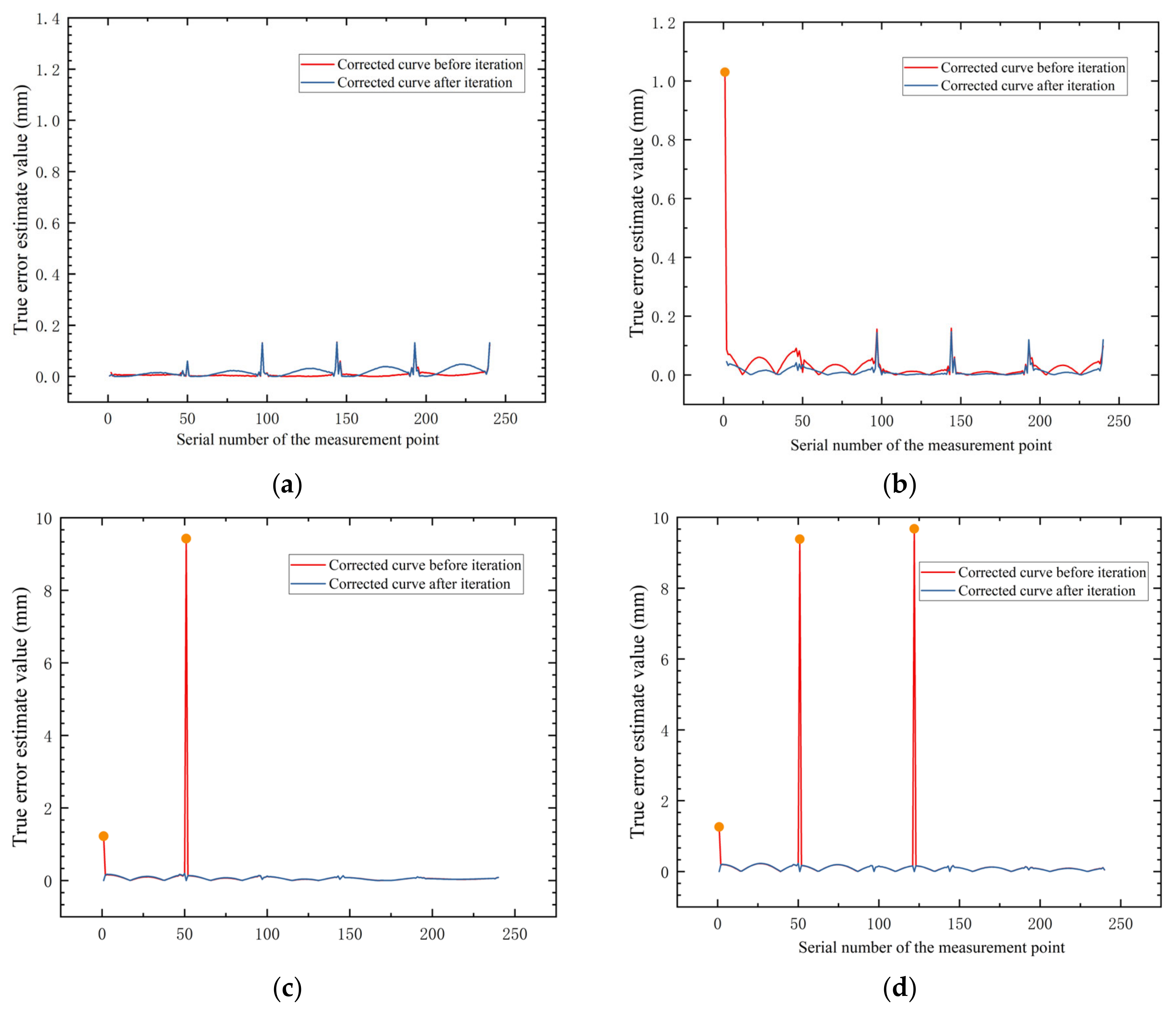
(2) By randomly inserting three gross error points, it was demonstrated that the cylindrical axis parameters calculated by the ISWLS method are stable when the data contain gross error points. The variation of cylindricity error is within 0.08 mm. The variation is smaller compared with the results without inserting gross error points, so the algorithm is able to resist gross errors.

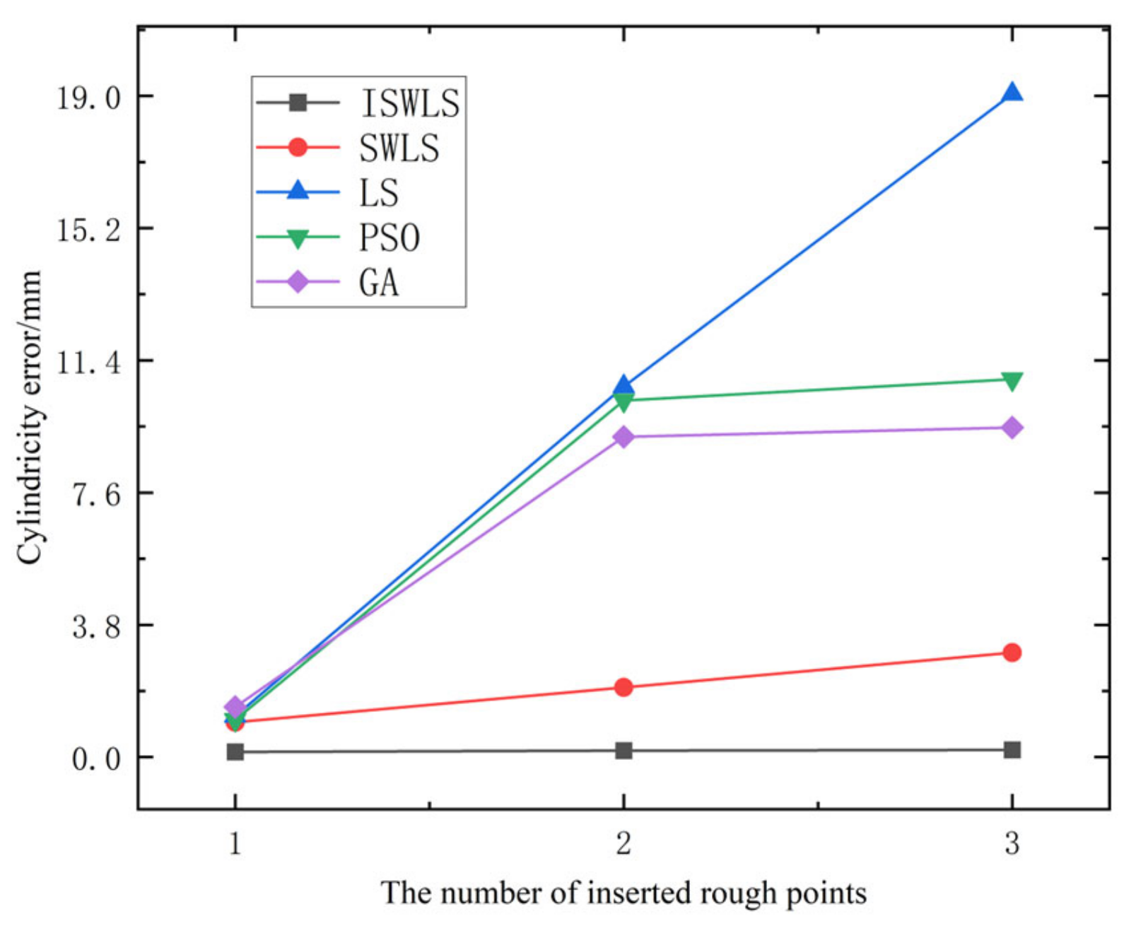
(3) In several experimental evaluations, compared with the particle swarm algorithm and genetic algorithm, the method in this paper took relatively less time and had faster computing power than the LS. In the experiment of inserting three gross error points, the LS method was most affected by the gross error points, and the standard PSO method and the standard GA method had less error increase in the cylindricity error value after the insertion of the second error point due to the advantage of the algorithm. The ISWLS method and the SWLS method have a certain resistance to gross errors. Compared with other algorithms, the cylindricity error assessment results did not increase significantly after inserting gross error points, the changes were relatively flat, and the ISWLS method was more resistant to gross errors than the SWLS method.

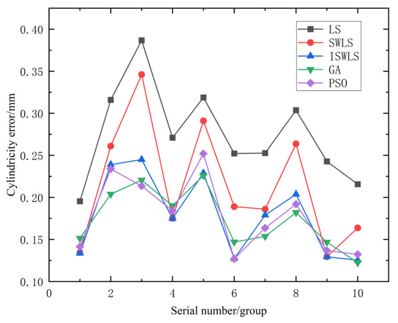
(4) The LS method, SWLS method, ISWLS, standard PSO method, and standard GA method were used to evaluate the model without inserting gross error points. Compared with other optimization algorithms, ISWLS has higher accuracy and stable arithmetic results with strong robustness. The results of the uncertainty evaluation experiments show that the GUM method results were verified by the MCM method, and thus the error uncertainty evaluation results are reliable. The ISWLS method has the robustness of the cylindrical error evaluation results. The algorithm can be extended to error evaluation.

References

1. Zheng, P.; Wu, J.Q.; Zhang, L.N. Research of the on-line evaluating the cylindricity error technology based on the new generation of GPS. Procedia Eng. 2017, 174, 402–409. [Google Scholar] [CrossRef]
2. Yang, Y.; Li, M.; Wang, C.; Wei, Q. Cylindricity error evaluation based on an improved harmony search algorithm. Sci. Program. 2018, 13, 2483781. [Google Scholar] [CrossRef]
3. Zhang, K.; Zhang, W.; Yan, W.Z.; Hou, H.S. Research on Evaluation and Uncertainty of Measurement of Circularity Errors via Neural Network Algorithm. Mech. Sci. Technol. Aerosp. Eng. 2019, 38, 428–432. [Google Scholar] [CrossRef]
4. Wen, X.L.; Song, A. Cylindricity Error Evaluation Based on an Improved Genetic Algorithm. Acta Metrol. Sin. 2004, 25, 115–118. [Google Scholar] [CrossRef]
5. Ambewadkar, G.N.; Gajre, S.P. Probe Path Planning for Flatness Measurement on Coordinate Measuring Machine Using Ant Colony Optimization. Adv. Eng. Forum 2021, 41, 6362. [Google Scholar] [CrossRef]
6. Tu, J.; Chen, H.; Liu, J.; Heidari, A.A.; Zhang, X.; Wang, M.; Pham, Q.V. Evolutionary biogeography-based whale optimization methods with communication structure: Towards measuring the balance. Knowl. Based Syst. 2021, 212, 106642. [Google Scholar] [CrossRef]
7. Zhang, Y.; Wu, M.; Fu, X.; Li, Q.; Gao, J. Reduced algorithm of laser measurement data for geometric parameters of ring forgings based on Artificial Immune Algorithm. Measurement 2019, 134, 527–538. [Google Scholar] [CrossRef]
8. Zhang, K.; Cheng, G.; Zhang, W. Evaluation of roundness error uncertainty by a Bayesian dynamic model. Measurement 2020, 155, 107565. [Google Scholar] [CrossRef]
9. He, G.Y.; Liu, P.P.; Wang, K. Evaluation of the cylindricity error based on the sequential quadratic programming algorithm. Mech. Sci. Technol. Aerosp. Eng. 2014, 33, 1845–1849. [Google Scholar] [CrossRef]
10. Wu, Q.; Zhang, C.; Zhang, M.; Yang, F.; Gao, L. A modified comprehensive learning particle swarm optimizer and its application in cylindricity error evaluation problem. Math. Biosci. Eng. 2019, 16, 1190–1209. [Google Scholar] [CrossRef]
11. Liu, D.; Zheng, P.; Wu, J.; Yin, H.; Zhang, L. A new method for cylindricity error evaluation based on increment-simplex algorithm. Sci. Prog. 2020, 103, 0036850420959878. [Google Scholar] [CrossRef]
12. Li, Q.; Ning, H.; Gong, J.; Li, X.; Dai, B. A hybrid greedy sine cosine algorithm with differential evolution for global optimization and cylindricity error evaluation. Appl. Artif. Intell. 2021, 35, 171–191. [Google Scholar] [CrossRef]
13. Wang, Y.X.; Wang, H.X.; Tian, H.H. Cylindricity Error Measurement and Evaluation Based on Step Acceleration Algorithm in Crankshaft Measuring Machine. MAPAN 2022, 2022, 1–10. [Google Scholar] [CrossRef]
14. Khattab, A.A.; Abouelseoud, Y.; Younes, M.A. Effect of Sampling Rates Variation during Cylindricity Error Evaluation. Int. J. Eng. Appl. Sci. 2019, 3, 257585. [Google Scholar]
15. Zaky, K.M.; Ghonem, A.A. Application of Robust Estimation Methods for Detecting and Removing Gross Errors from Close-Range Photogrammetric Data. Am. Acad. Sci. Res. J. Eng. Technol. Sci. 2019, 55, 111–120. [Google Scholar]
16. Yan, G.; Cen, M.; Li, Y. Gross error detectability and identifiability analysis in track control network for high-speed railway based on GEJE. J. Surv. Eng. 2020, 146, 04019020. [Google Scholar] [CrossRef]
17. Jia, N.N.; Ge, Y.H. Remainder reliability and robust estimation: A case study using twelve simulated leveling networks. Appl. Mech. Mater. 2013, 263, 3163–3167. [Google Scholar] [CrossRef]
18. Ge, Y.H. Research on the method of self-born weighted least square. Bull. Surv. Mapp. 2014, 8, 36–39. [Google Scholar] [CrossRef]
19. Survey Adjustment Subject Group, School of Surveying and Mapping, Wuhan University. Error Theory and Basis of Survey Adjustment; Wuhan University Press: Hubei, China, 2014. (In Chinese) [Google Scholar]
20. Oliveira, E.C.; Aguiar, P.F. Data Reconciliation in the Natural Gas Industry: Analytical Applications. Energy Fuels 2009, 23, 3658–3664. [Google Scholar] [CrossRef]
21. Ozyurt, D.B.; Pike, R.W. Theory and practice of simultaneous data reconciliation and gross error detection for chemical processes. Comput. Chem. Eng. 2004, 28, 381e402. [Google Scholar] [CrossRef]
22. Mian, S.H.; Umer, U.; Abdulhameed, O.; Alkhalefah, H. Prognosis and Multiobjective Optimization of the Sampling Plan for Cylindricity Evaluation. Math. Probl. Eng. 2020, 2020, 8201312. [Google Scholar] [CrossRef]
23. ISO 12180-2:2011; Geometrical Product Specifications (GPS)—Cylindricity—Part 2: Specification Operators. ISO: Geneva, Switzerland, 2021.
Figure 1. Diagram of cylindricity error.
Applsci 12 12319 g001
Figure 2. ISWLS cylindricity error algorithm evaluation process.
Applsci 12 12319 g002
Figure 3. MCM process for assessing measurement uncertainty.
Applsci 12 12319 g003
Figure 4. Cylindricity error measurement.
Applsci 12 12319 g004
Figure 5. ISWLS method cylindrical fitting.
Applsci 12 12319 g005
Figure 6. Cylindricity error evaluation comparison.
Applsci 12 12319 g006
Figure 7. Statistics chart of true error value when inserting gross error points. (a) No gross error point insertion. (b) Insert one gross error point. (c) Insert two gross error points. (d) Insert three gross error points.
Applsci 12 12319 g007
Figure 8. Influence of gross error on the results of different algorithms.
Applsci 12 12319 g008
Figure 9. Statistics chart of true error value when inserting gross error point.
Applsci 12 12319 g009