

Heat Transfer and Flow Characteristics of Coal Slurries under the Temperature Difference between Inside and Outside of the Channel
1
Frontier Scientific Research Centre for Fluidized Mining of Deep Underground Resources, China University of Mining and Technology, Xuzhou 221116, China
2
State Key Laboratory for Geomechanics and Deep Underground Engineering, China University of Mining and Technology, Xuzhou 221116, China
3
School of Mechanics and Civil Engineering, China University of Mining and Technology, Xuzhou 221116, China
*
Authors to whom correspondence should be addressed.
†
These authors contributed equally to this work.
Appl. Sci. 2022, 12(23), 12028; https://doi.org/10.3390/app122312028
Submission received: 9 October 2022
/
Revised: 20 November 2022
/
Accepted: 22 November 2022
/
Published: 24 November 2022
(This article belongs to the Topic Complex Rock Mechanics Problems and Solutions)
Abstract
:The pipeline transportation of coal slurries is always subject to a temperature difference between the outdoors environment and the fluid body. As slurries’ viscosity is typically temperature dependent, the flow is accompanied by the heat transfer. In this study, we used the CFD method to investigate temperature distributions and flow structures in straight and curved channels, which has not previously been investigated, according to our knowledge. First, the results demonstrate that the cooling process influences the flow structures along the stream. The fluid turns more sharply in the cooler fluid in the curved channel, the streamlines overlap at an earlier position within the bend, and the velocity maximum zone is wider. Cooling also has a significant impact on transverse flow. Because of the higher viscosity of the more cooled fluid and thus the difficulty of shearing the fluid in the stream-wise direction, the vorticity and strength of the vortex flow are greater. The fluid velocity at the central part of the channel points toward the inner wall at the beginning of the bend, resulting in an inner-wall biased temperature distribution, as the heat transfer is partially carried out by the fluid velocity. The central velocity points toward the outer wall at the end of the bend, resulting in the outer-wall biased temperature profile.
1. Introduction
Pipeline transportation has become the primary mode for transport of coal slurries, such as coal mud tailings or coal-water slurries. Because the rheological properties of these fluids, such as viscosity, are shear rate and temperature dependent due to the particle interaction, and components of clay [1,2,3] or polymers [4,5,6,7], their flow accompanied by the heat transfer process becomes rather complex when there is a temperature difference between the outdoor environment and the fluid body [8,9,10,11], which, in fact, is also encountered in some other geofluids [12,13,14]. Furthermore, the pipelines used for transportation in industries commonly consists of multiple straight tubes and bend sections. These bends induce a secondary vortex flow perpendicular to the main-stream direction, which is also complicated by the heat transfer processes.
In reality, even for Newtonian fluids in straight channels, the heat transfer and the accompanying flow characteristics in both laminar and turbulence regimes have been questioned for a long time [15,16,17,18,19,20,21,22,23,24,25,26,27,28]. Chandratilleke et al. carried our extensive studies on the flow and heat transfer in curved channels [29,30]. In one of their work, they used a helicity function and precisely described the three-dimensional secondary vortex structures in the rectangular channel bend [29]. Their simulations successfully determine the onset of hydrodynamic instability and the effects of the flow rates, rectangular aspect ratio and thermal fluxes on the flow characteristics and the heat transfer. In another work of Chandratilleke, they numerically simulated the flow in a rectangular bent duct with the wall heated, incorporating the buoyance force due to the heating in the formulas [30]. They found that under the wall heated, the Dean vortex in the curved channel is asymmetric compared to the symmetric vortex structure without wall heating, and the secondary vortex flow enhances the convective heat transfer. Yanase et al. used a spectral method and numerically calculated the flow in a curved rectangular duct, with the vertical outer wall heated but the inner wall cooled [31]. They found that at a smaller Grashof number, the flow turns from steady to periodic and then to chaotic pattern. Whereas, at a larger Grashof number, before the flow reaches the chaotic state, it experiences three steady-to-periodic cycles. At the periodic and chaotic states, the convective heat transfer is enhanced significantly by the secondary vortex flow. Zhang et al. numerically studied the flow and heat transfer in the curved wavy ducts [32]. They concluded that there exits an optimal combination of the wave amplitude and the wavy length to maximize the heat transfer. The flow resistance is more sensitive to the wave length compared to the amplitude because the wave length determines the frequency of the flow disturbance. Apart from these, the surface roughness has been proved to affect the heat transfer and flow behaviors. Wu et al. found that the efficiency of the heat transfer increases as the surface roughness or hydrophilicity increases, particularly at high Reynolds numbers [33]. However, as a cost, at these surface conditions, the pressure drop is larger.
For this research topic for non-Newtonian fluids, almost all studies are discussing the flow with heat transfer in geometries without bend. Dong et al. used a density-based topology optimization algorithm to calculate both Newtonian and non-Newtonian thermal fluids in rectangular channels, with the purpose of minimizing the pressure drop but maximizing the heat transfer [34]. The optimal design structures of the channels are different from Newtonian to non-Newtonian fluids, and this difference is maximized below Re = 0.01. Non-Newtonian fluids always perform better in heat transfer, but at the expense of a higher pressure drop. Shojaeian et al. studied the flow of non-Newtonian fluid in circular-cross-section channels under a thermal isoflux imposed on the channel wall, with the consideration that the viscosity and the thermal conductivity are functions of the temperature [35]. They gave an analytical solution of the fully developed flow and found its deviation from the one using the temperature-independent fluid properties that could reach 32%. Sayed-Ahmed et al. used a finite element method to study the flow of power-law fluids with different index numbers in an annular gap between two coaxial rotating cylinders [36]. The boundary condition of the simulation is an adiabatic and stationary outer wall and an inner wall with a constant temperature and angular velocity. They found that the increase of or the thermal conductivity causes the decrease of the average Nusselt number. For the shear thinning fluids (index smaller than one), the average Nusselt number is obviously affected by the viscosity parameter. With the elasticity considered further, Nóbrega et al. theoretically calculated the flow of a Phan-Thien–Tanner fluid in a channel with a temperature difference between the wall and the fluid from the inlet [37]. The results correct the expressions of the Nusselt number and the friction factor for the non-Newtonian fluids. The corrections are shown to be dependent less on the viscous dissipation but largely on the elasticity that is represented by the Weissenberg number. Barkhordari et al. used control volume finite difference method to solve the flow of non-Newtonian fluids described by Ostwald–de Waele power law in circular channels, but with the consideration of the wall slip [38]. The results demonstrate that the change on the Nusselt number due to the slip and no-slip is particularly pronouncing for higher power index. As the slip coefficient increases, the center-line velocity decreases but the Nusselt number increases.
The flow of non-Newtonian fluids in channel bends has been studied systematically, but with no heat transfer involved. Li et al. used lattice Boltzmann method to simulate the flow of Herschel-Bulkley fluids in 90° bent circular channels, with the power-law index, yield stress and the curvature radius of the channel varied [39]. They concluded that the flow resistance increases with the power index, yield stress and the curvature radius, while the additional pressure loss due to the bend reduces with the curvature radius. The bend introduces the Dean vortex secondary flow, whose intensity decreases as the yield stress or the power index increases, because the larger viscosity hinders the centrifugal force. Roberts et al. derived an analytical expression for the velocity profile of a Bingham fluid in a two-dimensional curved pipe [40]. As the Bingham number increases, the fluid velocity and stress at the inner wall decreases. For a fixed Bingham number, the width of the unyielded plug is smaller for the larger curvature. Marn et al. numerically solved the flow of shear thickening fluids in a pipe with curvature [41]. Since the flow in the bend part is not fully developed when the curvature radius is small, the numerical friction factor was demonstrated to be much greater than the classical empirical predictions given by White and Mishra-Gupta. They concluded a new experienced expression for the friction factor based on two shear thickening rheological models: the power-law model and Quadratic model, respectively.
In this study, we used CFD approach to simulate the flow of non-Newtonian coal slurries in straight and curved channels at different conveying rates and under different thermal isoflux on the wall. In the formulas employed in the simulations, the thermal conductivity of the fluid is only a function of temperature, while the viscosity is dependent on both shear rate and temperature. In straight channels, we studied the temperature distribution at the cross section, and the pressure drop that is affected by the temperature since the viscosity changes as the heat transfer processes. In the curved channels, we looked at the secondary flow structures in the bend and the impacts of heat transfer, which, to our knowledge, have not been specifically addressed in earlier studies.
2. Simulation Method
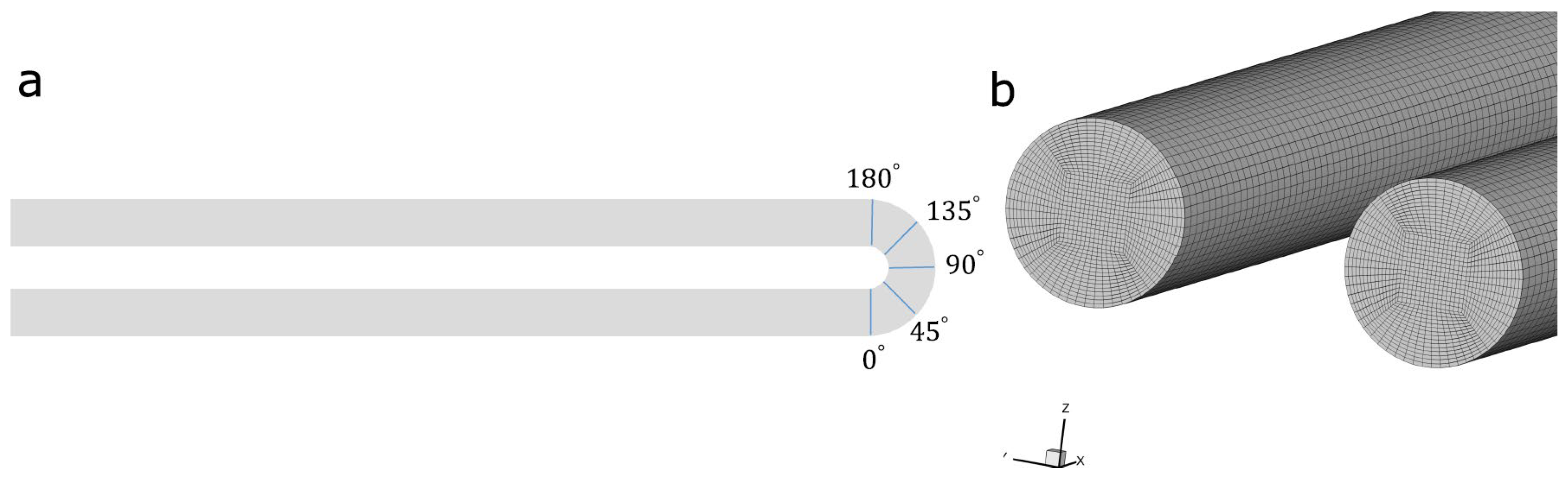
The simulations were carried out using the Ansys Fluent software [42]. There were three different types of circular cross-section channels used. One is a one-meter-long straight channel, and the other is 1.5-m-long. The third channel is a U-shaped one (Figure 1a), with two straight arms of 1 m length, a 0.25 m middle curved part of the outer-wall perimeter, and a 0.05 m wall–wall separation between the two straight parts. All of the channels have the same diameter of 55 mm. The structured mesh of the three channels has approximately 600,000 nodes (Figure 1b), and we tested a mesh with more nodes that would produce nearly identical results. The simulations’ boundary conditions are an inlet velocity and a constant temperature for the incoming fluid, zero pressure and an open-to-the-air temperature at the outlet, and no-slip on the wall with a constant temperature . Two inlet velocities and two temperatures were imposed for each channel. The Bingham model describes slurry viscosity, and the Arrhenius model [43] reflects temperature influence:
Here, is the yield stress, is the consistency index, and is the temperature whose unit is K. The values of and are referred from [44], in which the rheological properties of coal slurries are systematically measured using a rheometer. The thermal conductivity of the slurry is referred to [37]:
where , , and . The temperature-dependent viscosity and thermal conductivity were written into Fluent through a User Defined Function. The Reynolds numbers , as defined by [39], are approximately 12 and 24, respectively, for the two flow rates, demonstrating that the turbulence can be neglected. Here, is the density of the fluid and is taken as in the simulations.
The equations to be solved for the incompressible flow of non-Newtonian fluid are the conservation of mass
linear momentum
and thermal energy
is the specific heat, is the velocity in the direction, is the fluid pressure, and is the stress tensor.
3. Results and Discussions
3.1. Straight Channels
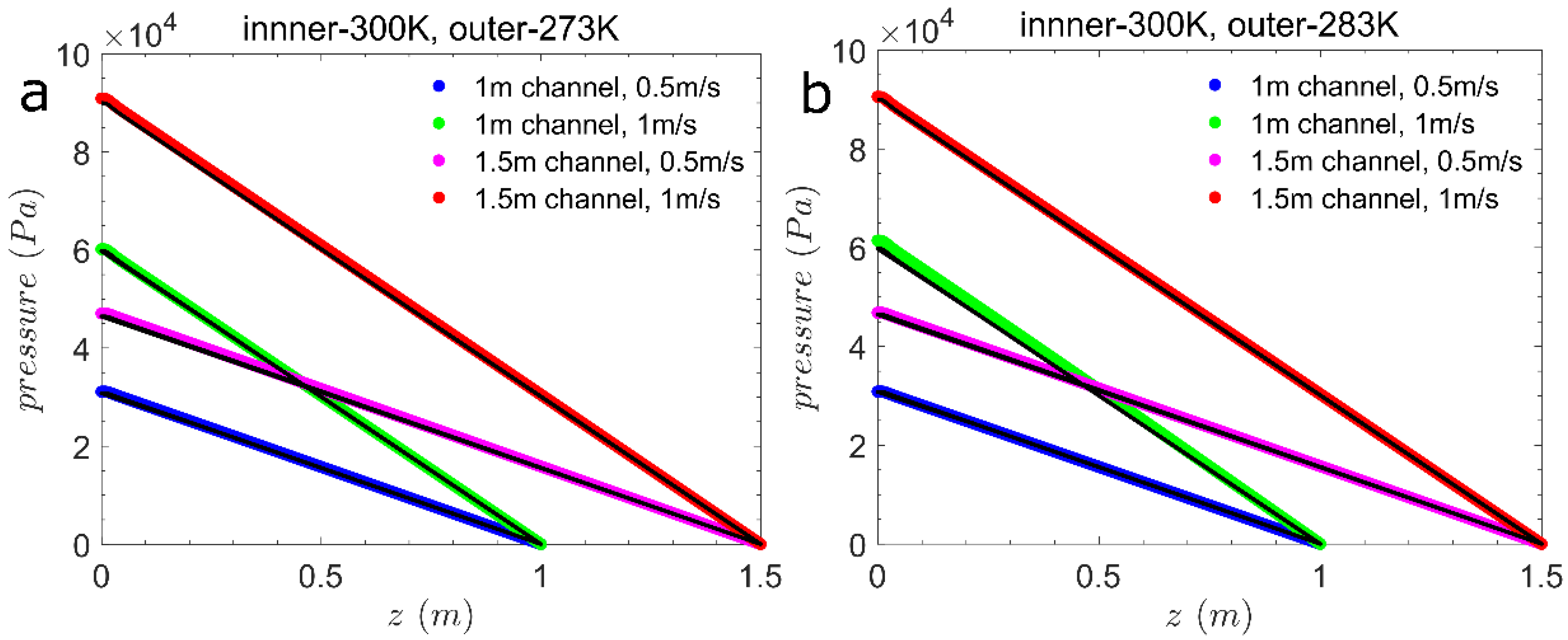
Figure 2 depicts the pressure in the straight channels along the axial line. Because of the increased viscosity caused by cooling operations, the pressure values at the cooling temperature boundary conditions are frequently slightly higher than those without cooling. The pressure values at the larger temperature difference’s boundary conditions are slightly higher than those at the smaller temperature difference, with an exception of one case in the 1 m channel at and a wall temperature of 273 K, as shown by the green line in Figure 2a. Furthermore, as the channel length increases, the pressure rises slightly because the fluid is chilled further, increasing its viscosity. It appears that the fluid inlet velocity has no effect on the pressure readings. However, it has an effect on the temperature distributions, which will be discussed in more detail later.
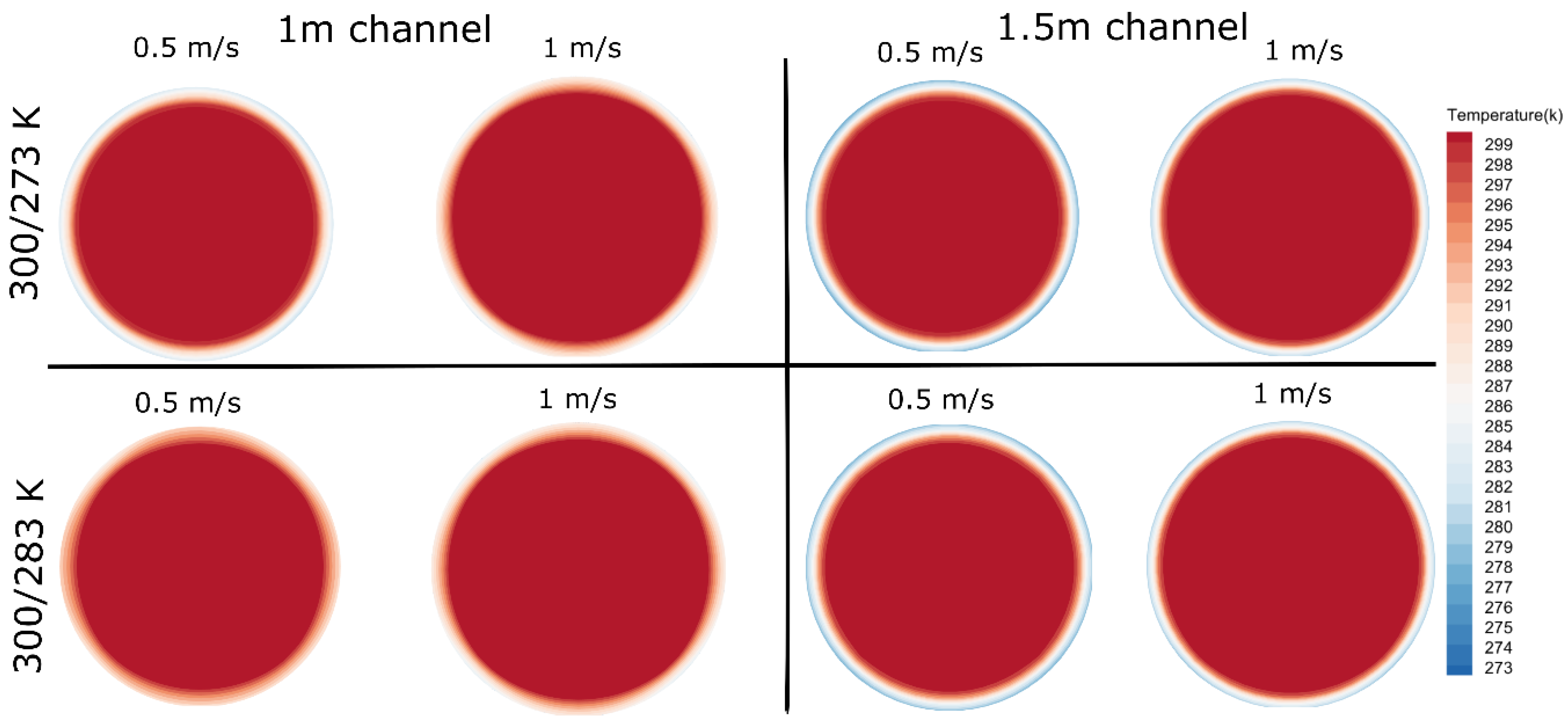
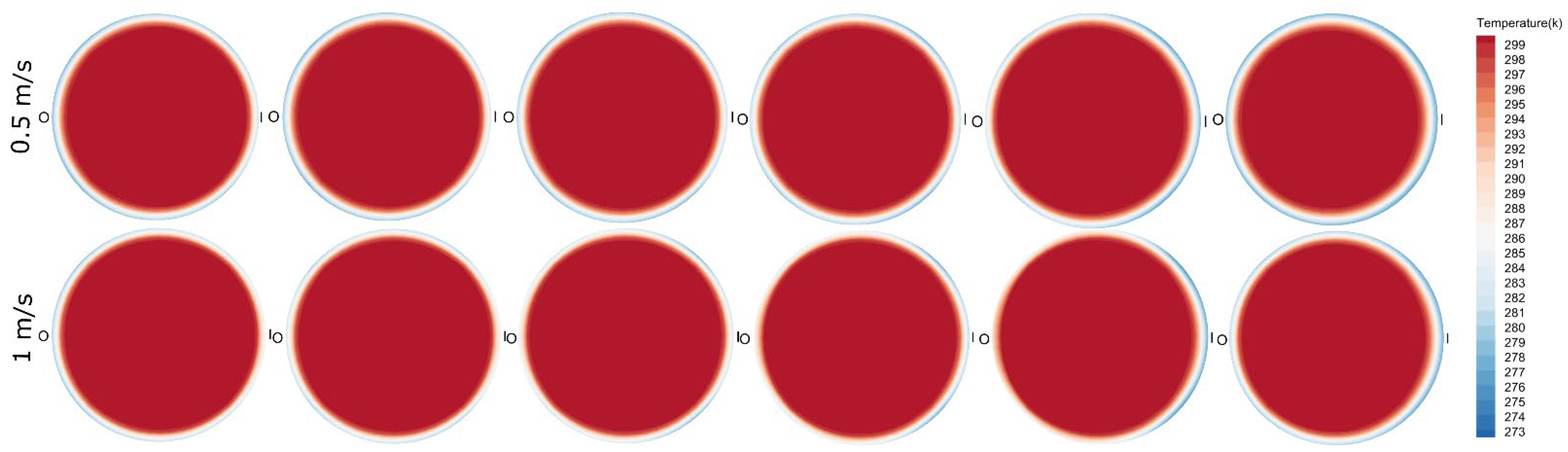
Figure 3 depicts the temperature profiles at the channel outlet. The more cooled slurry has a slightly narrower central high-temperature core than the less cooled slurry. Again, increasing the channel length causes more heat transfer from the fluid body to the wall, resulting in a more-slender temperature maximum zone. These images also demonstrate the effect of flow rate on heat transfer, which is greater at lower flow rates and is represented by the wider low-temperature ring near the wall. Because the flow in straight channels is always along the axial direction, there is no transverse flow, and thus the heat flux is merely due to thermal conduction rather than the heat carried by the transverse fluid velocity. As a result, the heat transfer increases as the fluid stays for a longer time or at a lower flow rate.
3.2. U-Shaped Channel with a Larger Temperature Difference
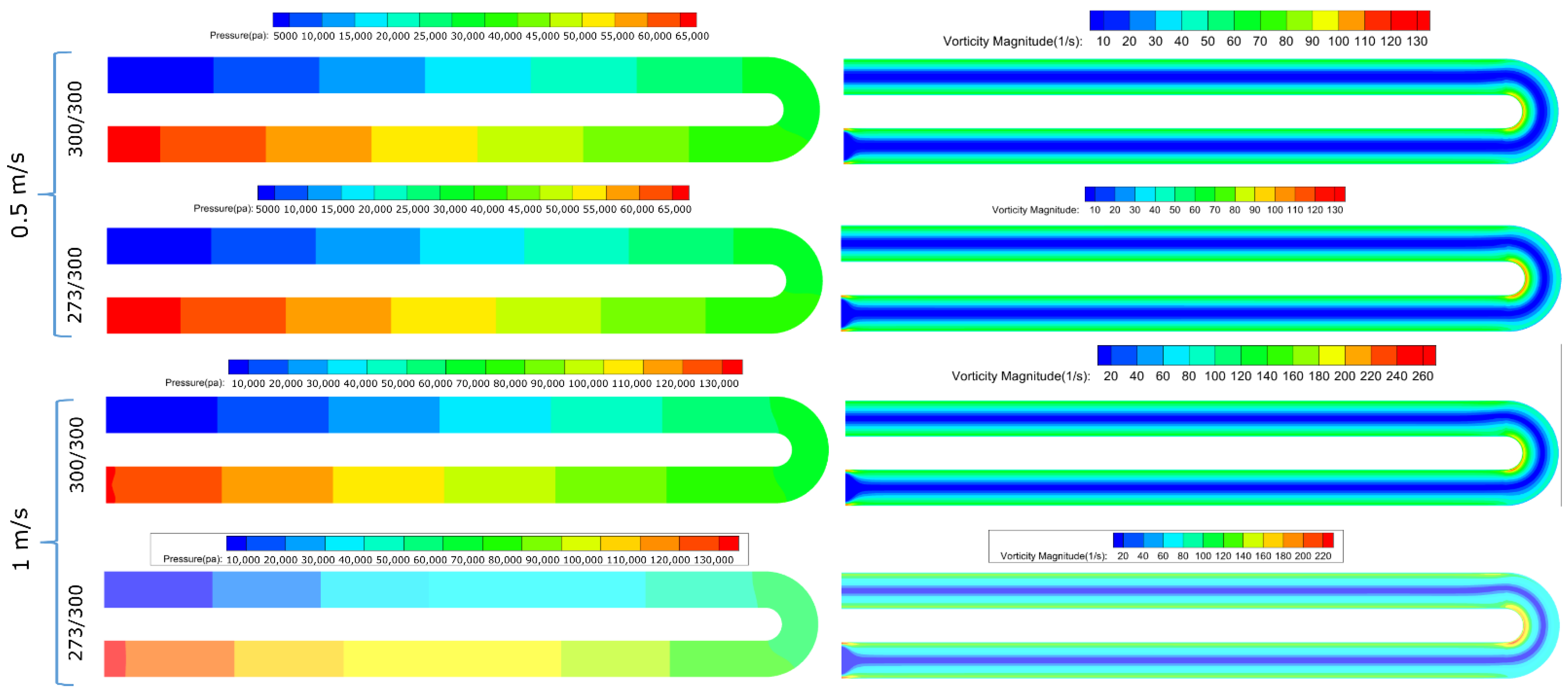
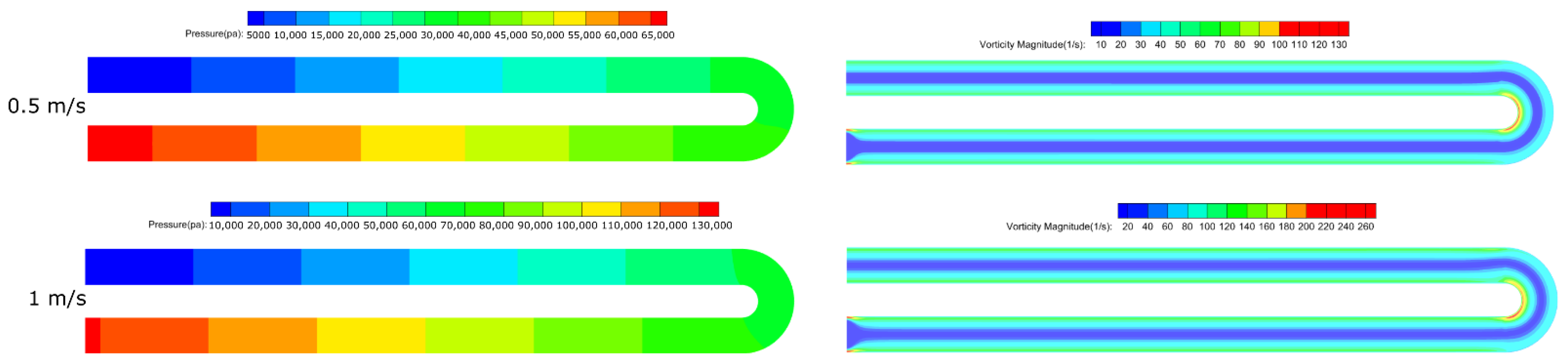
In this section, we will demonstrate the results at a temperature difference of 300–273 K between the incoming fluid and the channel wall of the U-shaped channel. Figure 4 shows the pressure and the vorticity at the middle-height plane of the channel at uncooling and cooling temperature boundary conditions and at different flow rates, respectively. Comparing the cooling flow and the uncooled flow at the lower flow rate, there is no obvious difference. However, at the higher flow rate, both the pressure and the vorticity distributions change as the cooling processes. The pressure for the uncooled fluid decreases more gently along the channel, whereas the pressure of the cooled fluid drops more suddenly, especially behind the bend. From this, we can suspect that the cooled and quicker fluid dissipates the energy most at the bend, which can be partly evidenced by the fact that the vorticity of the cooled fluid is generally larger in space than that of the uncooled fluid, although the maximum vorticity of the cooled fluid is smaller. If we compare the data at the same temperature conditions but at different flow rates, the uncooled results demonstrate no obvious change, whereas the cooled fluid does. For the cooled fluid, as the flow rate increases, the pressure drops more sharply, and the vorticity is universally larger, the latter of which suggests that the secondary flow for the quicker fluid is stronger. The following results of the transverse flow structures will verify this.
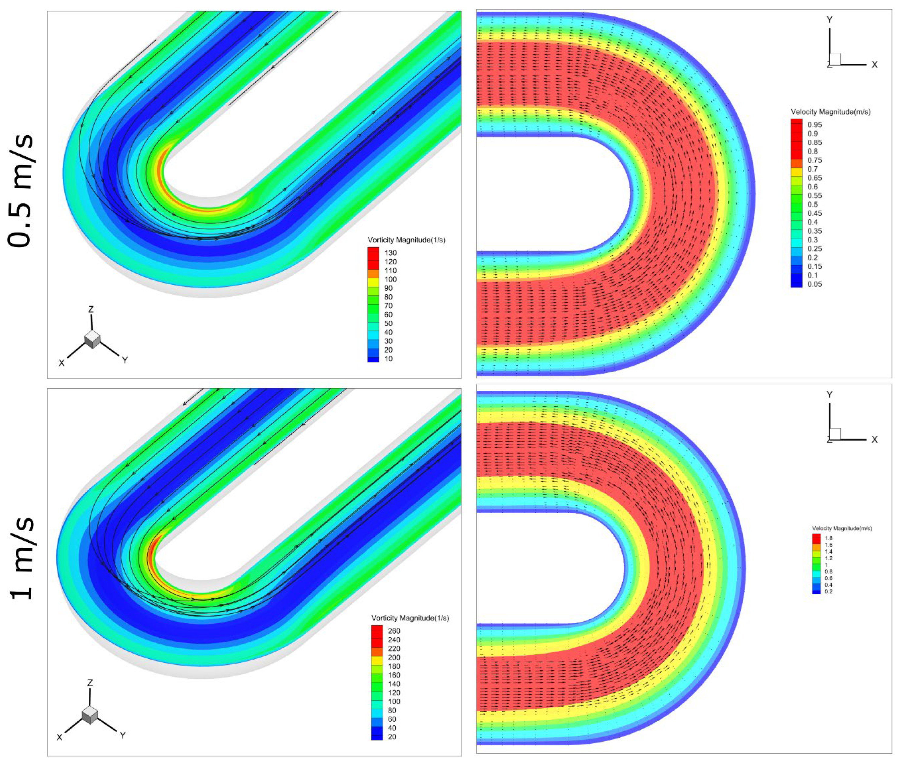
To represent the flow details in the bend, Figure 5 shows the 3D streamlines, vorticity magnitude, velocity magnitude, and the velocity vector arrows on the middle-height plane. Again, let us first compare the results at the same flow rate but under different temperature conditions. In the cooled fluid, the maximum vorticity value seems to decrease, and the overlap of the streamlines occurs at an earlier position, which corresponds to the earlier twisted velocity vectors. As the fluid processes cool, the maximum velocity zones become wider. Secondly, let us compare the results at the same temperature conditions but at different flow rates. As the flow rate increases, the vorticity at the inner wall within the bend is less symmetric, the maximum velocity zone shrinks, and the turn of the flow is larger. Interestingly, at the higher flow rate, and especially in the cooled fluid, the flow deflects towards the outer wall behind the bend but then recovers slightly back to the inner wall, which is presumably because that the more viscous fluid has more motion in the transverse direction since it is more difficult to be sheared in the stream direction. This will be confirmed by the results of the transverse flow structures discussed in the following.
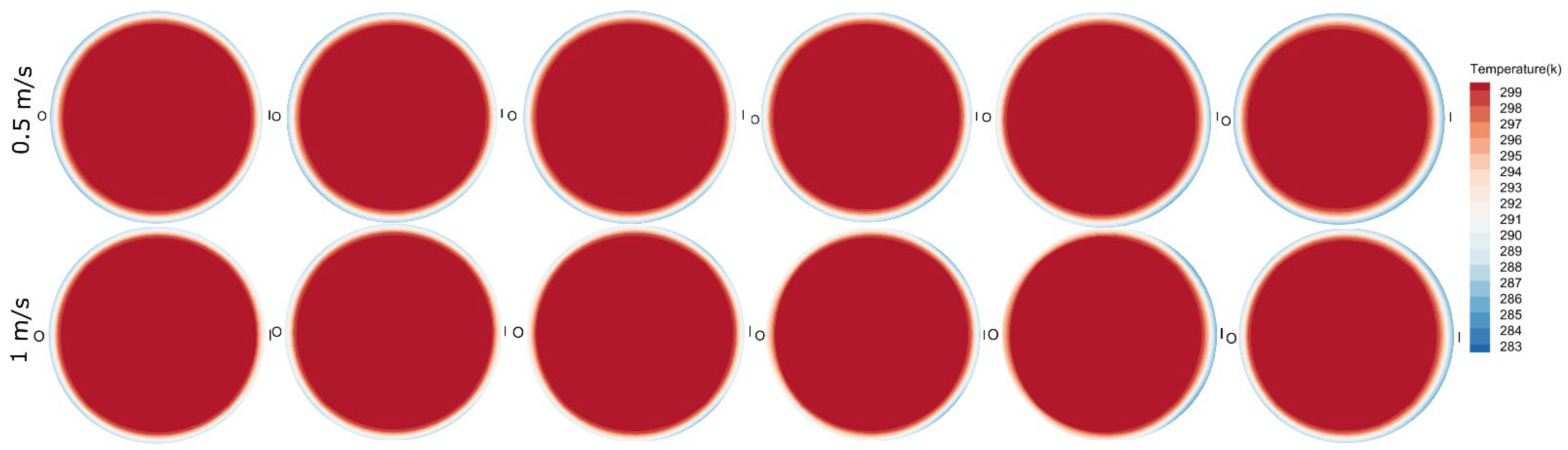
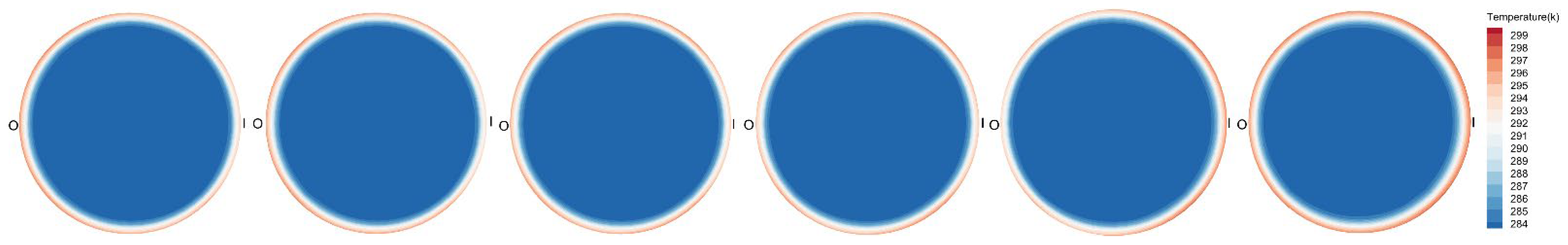
Figure 6 displays the distributions of the temperature at the five sections and the outlet plane of the U-shaped channel. From the left to the right, the order of the sections is from the inlet to the outlet. In the curved channel, the heat transfer differs from that in the straight channel since there is transverse flow in the curved one and thus the heat transfer also has the component carried by the fluid velocity. First, at the lower flow rate, it can already be observed that the temperature distribution is asymmetric about the inner and outer walls. As the fluid enters the bend, of which the result is shown in the left column, the temperature on the inner wall side is larger than on the outer wall side, since, at this section, the fluid velocity points to the inner wall (Figure 7, left column). At the 135° section (the fourth column), the temperature almost returns to the symmetry, which is pulled back by the outer-wall pointed fluid velocity at the central part of the cross-section. In the 180° section, the temperature is completely biased on the outer wall side. In contrast, when the flow rate is higher, the temperature distribution is more asymmetrical, whether it is toward the inner wall or the outer wall, and the symmetric distribution occurs earlier, at the 90° section, meaning that the outer-wall pointed central flow is stronger than that at the lower flow rate. Another difference is that at the outlet for the quicker flow, the temperature is still biased towards the outer wall due to the less decayed secondary flow.
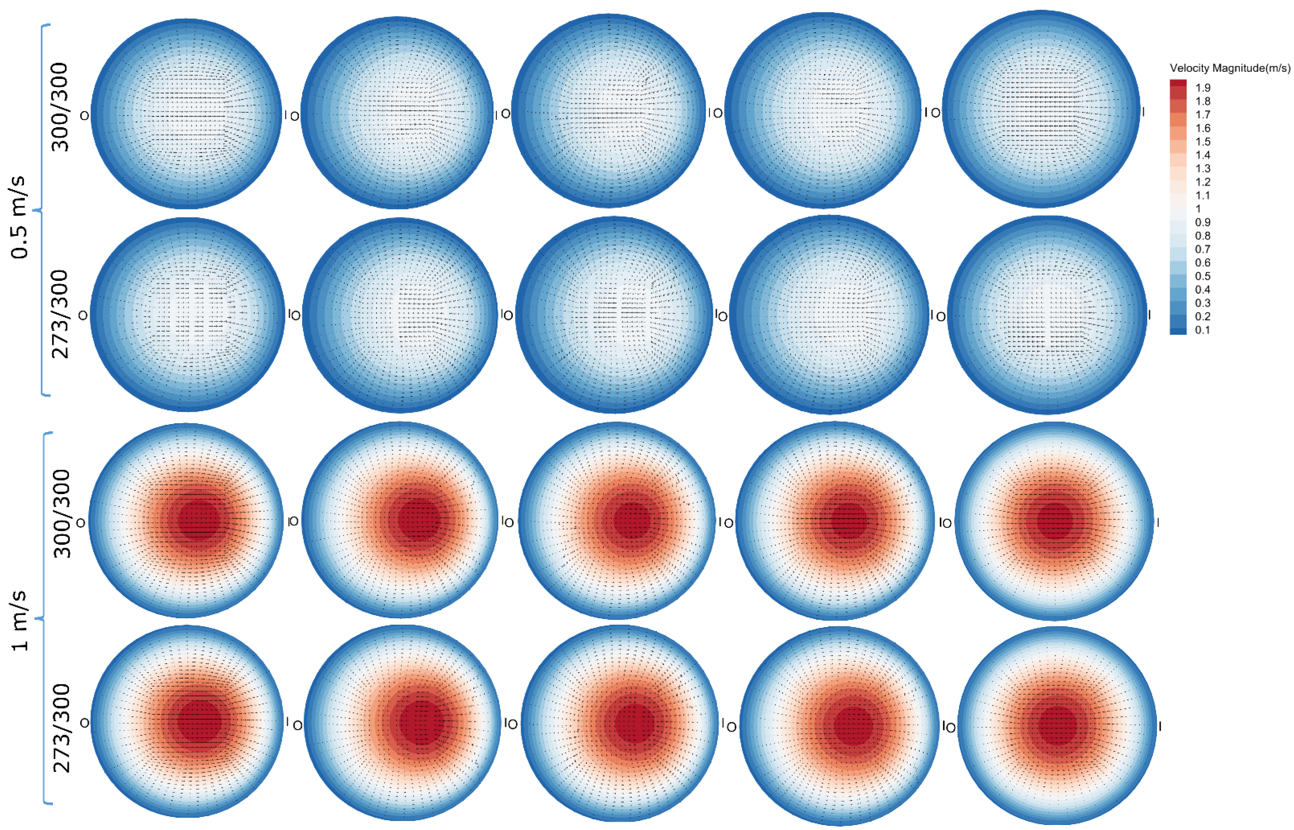
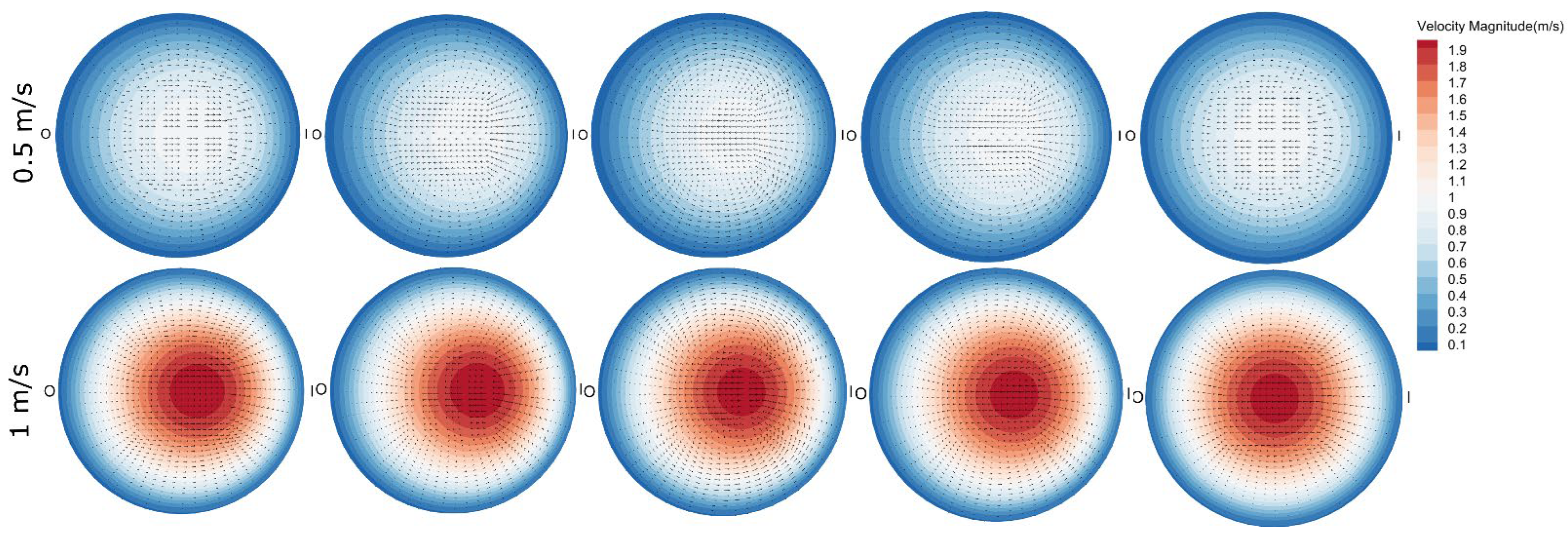
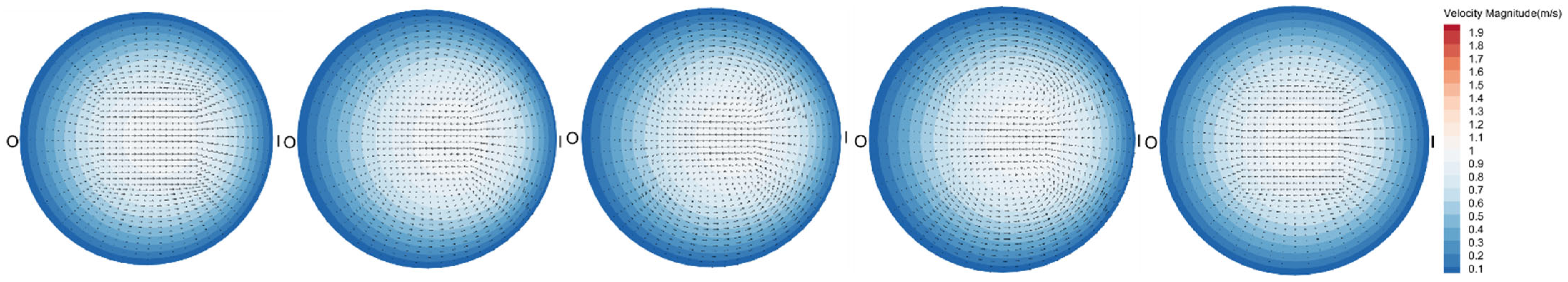
Figure 7 demonstrates the velocity magnitude and the vector arrows for the five sections of the U-shaped channel. We can observe that, except for the 180° section, the maximum velocity zone is always closer to the inner wall, since at the inner wall side the fluid travels a shorter distance. Initially, let us compare the results at the same flow rate but with the different temperature boundary conditions. First, the cooled fluid shows a much stronger secondary vortex flow regardless of the lower and higher flow rates, which corresponds to the larger vorticity values observed in the cooled fluid (Figure 4). To understand this, the cooled fluid has a larger viscosity and thus the fluid is harder to shear in the main-stream direction. However, the fluid’s velocity has to be that large. As a result, more velocity is in the transverse direction and converts to the secondary flow. Second, we compare the results at the same temperature boundary conditions but different flow rates. Obviously, as the flow rate increases, the secondary flow is stronger, and the deflection of the velocity maximum zone is larger.
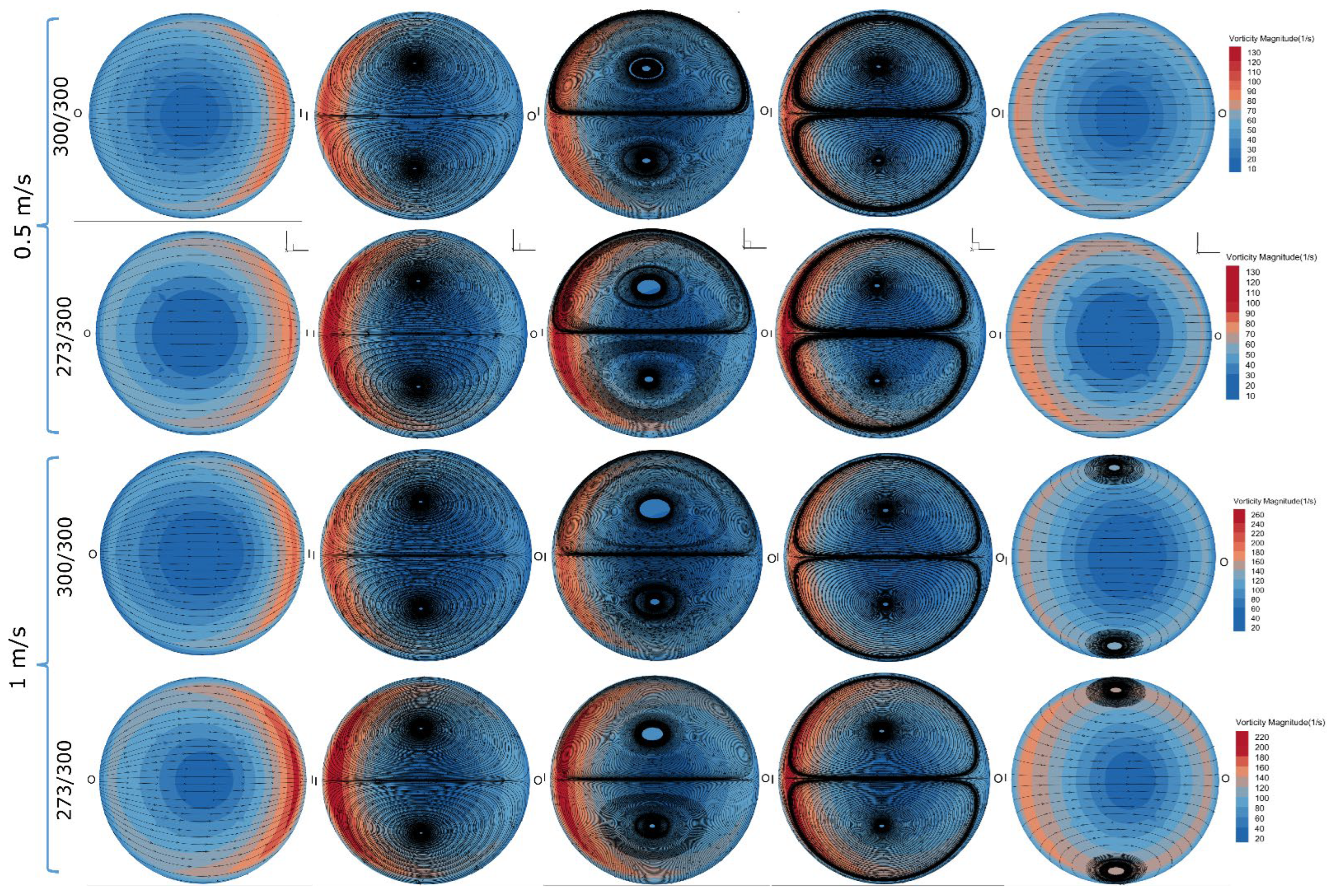
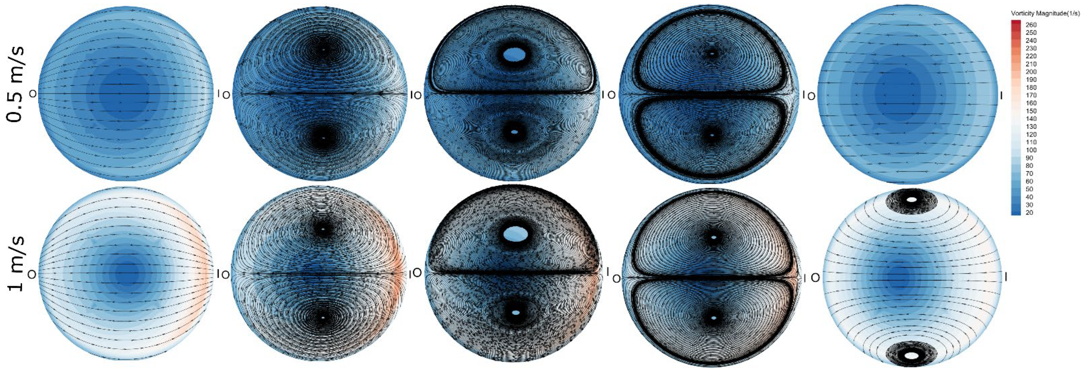
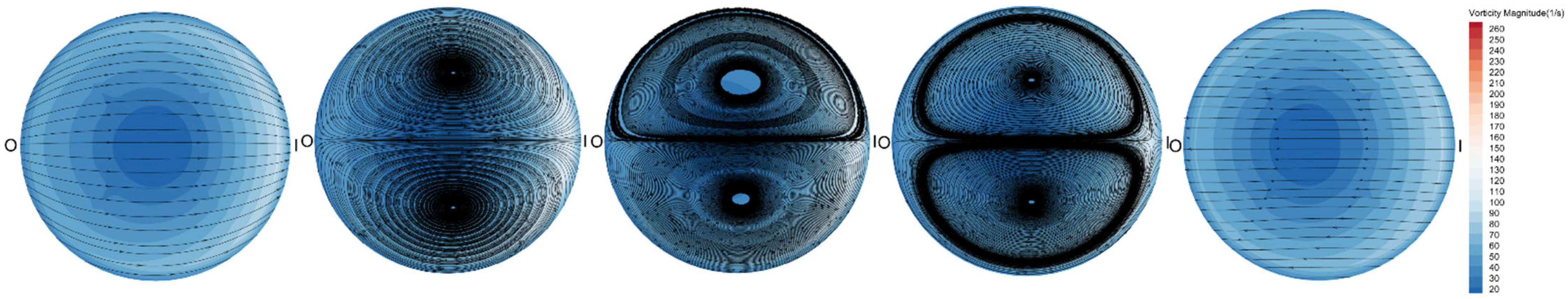
Figure 8 shows the vorticity profiles in the five sections of the channel. In all sections, the maximum vorticity is always biased towards the inner wall. At the beginning of the bend, the flow points to the inner wall, whereas in the rest sections, the central flow points to the outer wall. At the end of the bend and at the higher flow rate, the vortex flow is still there, whereas at the lower flow rate, the vortex has decayed out. Referring to the cooling, again, the same as the results shown in Figure 4, the vorticity values in the cooled fluid are larger, and the streamlines are denser, meaning the stronger vortex flow.
3.3. U-Shaped Channel with a Smaller Temperature Difference
This part describes the heat transfer and the flow characteristics in the U-shaped channel, at the temperature boundary conditions of 283 K on the wall and 300 K of the incoming fluid at the inlet. Figure 9 shows the pressure and the vorticity magnitude at the middle-height plane of the channel. The inlet–outlet pressure drop values show no change as the wall temperature changes, compared to Figure 4. However, the vorticity values change. At the lower flow rate, the vorticity shows a narrower minimum zone compared to the one in the more cooled fluid, meaning that the fluid in this case is less rigid since the fluid is less cooled and thus the viscosity is smaller. At the higher flow rate, the maximum vorticity is larger than that in which the fluid cools more, again showing that the fluid is less rigid. Another noticeable phenomenon is that, at both lower and higher flow rates, the vorticity is less symmetric than that of the more cooled fluid, which also reflected this. From the streamlines, vorticity, and velocity magnitudes/vectors displayed in Figure 10, the less cooled fluid shows a more asymmetric vorticity distribution at both flow rates. Moreover, the flow turns more gently and the maximum velocity zone is more oblique, together with the later overlap of the streamlines in the curved part, meaning that the deflection of the less cooled fluid is easier and smoother. Ass the flow is faster, it seems that the maximum velocity zone is even oblique. The disappearing velocity vectors at the strongly curved points indicate that there should be a strong cross-section secondary flow at these positions.
The temperature profiles at the five sections and the outlet plane of the U-shaped channel are shown in Figure 11. Overall, compared to the cases of the larger temperature difference, the distribution is more symmetrical because of fewer heat transfer processes, and at the higher flow rate, it is even more symmetrical. Again, at the beginning of the bend, the temperature at the inner wall side is higher due to the inner-wall-pointed velocities (Figure 12), and thus the heat is transferred from the outer wall to the inner wall. From the 0° section to the 180° section, the temperature profile biased to the inner wall converts to the profile biased to the outer wall due to the stronger and stronger outer-wall-pointed flow at the central part of the sections. At the higher flow rate, at the outlet plane of the channel, the profile is still biased to the outer wall, which is attributed to the vortex flow that has not decayed completely.
The velocity magnitudes, vectors, and the vorticity magnitudes and streamlines are shown in Figure 12 and Figure 13. As the fluid turns more gently and it starts to turn at an earlier point, the velocity maximum zone at the 0° section deflects less towards the inner wall, particularly at the higher flow rate, and similarly, the flow at the 145° section deflects less towards the outer wall. However, the maximum velocity values are not changed as the temperature changes, but the maximum velocity zone is obviously larger compared to the results in the more cooled fluid at the same flow rates. At the end of the bend, at the higher flow rate, the flow temporarily deflects towards the outer wall as an inertia, and this deflection is closer to the outer wall compared to the flow in the more cooled fluid at the same flow rate, due to the smaller viscosity and thus the easier twist. From the results of the vorticity and the streamlines, the vorticity on the cross sections in the less cooled fluid is smaller and the streamlines at the channel center are generally looser because the fluid’s viscosity is smaller and the fluid is easier to shear in the stream-wise direction.
3.4. Pressure Loss and Energy Dissipation Due to the Bend
In industries, it is important to accurately predict the pressure drop in the pipe bend for optimizing the design of the complex geometries of the pipes. For the fully developed flow in the bend with a large curvature radius, the friction coefficient has a ready-use expression. However, in the bend with a small curvature radius, such as the one in the present article, the flow is not fully developed. Moreover, our fluid is plastic and there is an unyielded plug at the center of the channel. All these factors may induce abnormal phenomenon, and the existing formula of the friction may not be applicable. Therefore, this section will analyze the pressure loss, friction coefficient, and the energy dissipation rate induced by the bend, to compare with the previous studies and to provide comprehensive understandings.
The extra pressure loss induced by the bend is the difference between the total pressure drop and that of a straight pipe with a same length, which is defined by [41]:
is the total pressure drop of the U-shaped channel, is the pressure gradient of the straight channel with the same length, is the length of the straight part of the U-shaped channel, and is the length of the bend part. Here, we employ a dimensionless pressure loss coefficient to represent the influences of the flow rate and the temperature. The values of are summerized in Table. 1. When calculating , we used the following relation between and for the Bingham fluid [45]:
and are the channel radius and the radius of the unyielded plug, respectively. is the average flow velocity. As Table 1 shows, surprisingly decreases with the flow rate, and increases as the fluid cools more because of the increase in the viscosity. According to the previous studies of laminar flow of non-Newtonain fluids in a bend [32], it is reasonable to suppose that the pressure drop in the bend is almost totally associated to the energy dissipation rate due to the viscosity. Herein, we took along the horizontal diameter of the cross section at the middle of the channel as the average to calculate the total energy dissipation rate in the whole bend part:
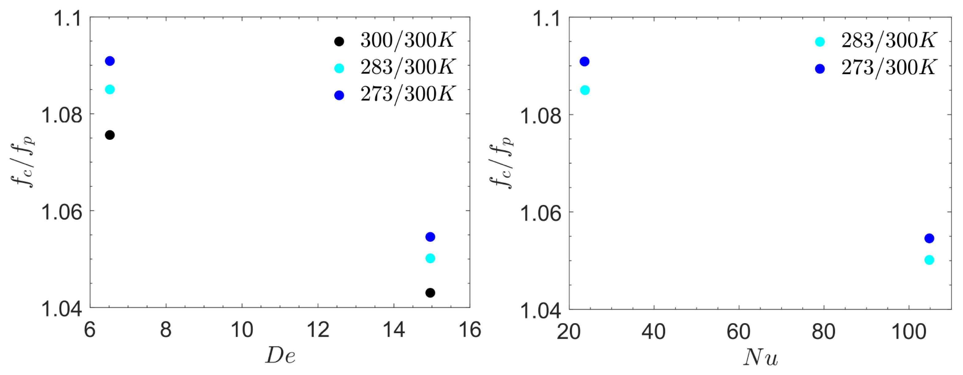
where is the vorticity vector and is the volume of the whole bend part of the channel. Moreover, we made dimensionless through dividing it by , in which is the volumetric flow rate. The values of in different cases are listed in Table 2, and it shows the same tendency as , which confirms our supposition that the viscosity mainly dissipates the energy in the bend. Actually, in the early studies, it was widely accepted that the energy loss due to the bend, which was sometimes represented by the friction coefficient , increases as the Dean number that is propertional to the fluid velocity. For example, Singh and Mishra gave the expressions of the friction coefficient: and for Newtonian fluids [46]. Marn concluded for power-law fluids [41]. Here, is the friction coefficient of the straight pipe with a same length. , in which is the curvature radius. However, in the present study, we obtained the converse relation between and , as observed more clearly in the plot of Figure 14. We speculate that this is due to two effects: one is the special rheology of our fluid, particularly the plasticity–yield stress; the other is the not fully developed flow in the strong curvature. At the lower flow rate, the yield stress fluid flows with an almost unyielded plug at the central part of the pipe, resulting in a nearly infinitely large viscosity [45]. Nonetheless, there is still a weak Dean vortex secondary flow inside the plug [47]. As the flow rate increases, the width of the plug shrinks, and in the places where the plug locates at the lower flow rate, the infinite viscosity sharply reduces to an intermediate value. In contrast, the magnitude of the squared vorticity increases by a smaller magnitude. Remember that in our case, the vorticity always weighs more on the inner-wall side of the channel (Figure 8 and Figure 13). Compared to the outer-wall-weighted vorticity in the fully developed flow in a smaller curvature, the vorticity in our case is relatively smaller and hindered due to the outer-wall pointed fluid velocity. Therefore, the decrease in the viscosity is greater than the increase in the squared vorticity, and the variation of the viscous energy dissipation rate with the flow rate follows that of the viscosity, which decreases as the flow rate increases. At least, this is true in the range of the flow rates in the present study. It is uncertain to predict if the relation between the energy loss and the flow rate would return to the positive correlation at even higher flow rates, at which the decrease of the viscosity might be less than the increase in the squared vorticity magnitude. Because in engineering, the coal slurries are not conveyed at higher rates, that range is not discussed here. Moreover, the turbulence begins to arise at the higher rates, and the energy loss would be not only due to the viscosity, which would make the problem more complicated.
We also plot the friction coefficient as a function of the Nusselt number that represents the ratio of the convective heat transfer to the conductive transfer, shown in Figure 14. When calculating , similar to , we selected the horizontal radius near the outer-wall side of the cross section at the middle of the U-shaped channel as representative of the whole bend part:
is the average velocity in the main heat transfer direction (positive x) outside the temperature-plug region (for example, Figure 6 and Figure 11). is the temperature difference between the fluid body and the pipe wall. is the temperature gradient in x direction. As shown in Figure 14, again decreases as increases, since is similar to , which is proportional to the flow rate. From both plots in Figure 14, we notice that the deviation of from different thermal fluxes is reduced at larger or , implying that the pressure loss is more affected by the temperature in the slower flow.
3.5. Inverse Thermal Flux from the Wall to the Fluid
In some real circumstances, the slurry’s temperature is lower than the environment due to the hot weather, and as a result, the thermal flux flows from the pipe wall to the inner slurry. We simulated such a case, in which the temperature on the pipe wall is constantly 300 K whereas the slurry coming from the inlet is 283 K. The inlet velocity is 0.5 m/s. Figure 15 shows the temperature distributions at the five slices in the bend and the outlet. Under such a thermal boundary condition, the heat flux is from the wall to the fluid. Therefore, opposite to the cases in the cooler pipe, the lower temperature is biased to the inner wall at the beginning of the bend, while it is biased to the outer wall at the end of the bend.
The velocity magnitudes and the vectors at the five cross sections within the bend are shown in Figure 16. Compared with the results in the case of the inverse temperature flux at the same flow rate (Figure 12, upper row), because of the lower temperature and thus the higher viscosity of the fluid in this case, the central velocity becomes smaller. The vorticity distributions (Figure 17) are not quite different from the case with the inverse thermal flux (Figure 13, upper row). There is only a minor deviation that the streamlines are denser near the channel edge in in this case with 300/283 K, especially at the 45° section. The same phenomenon is also observed, comparing the cases of 273/300 K and 300/300 K at the same flow rates (Figure 8). This is mainly due to the almost unyielded plug flow at the center of the cross section. The fluid’s temperature and the viscosities are lower in the case of 300/283 K compared with the case of 283/300 K. Thus, the plug is wider and the fluid within the plug is more rigid, resulting in a greater difficulty of creating a rotational flow inside, and therefore the most rotational flow is outside the plug and near the edge.
Comparing both cases of 283/300 K and 300/283 K with the case of 300/300 K (Figure 7, upper row), it is found that the deflection of the minimum or the maximum vorticity core is switched to different sides from the case with zero thermal flux to the cases with non-zero thermal flux, regardless of the dirction of the heat transfer. Under a temperature difference, at the 0° section, the minimum vorticity is always biased to the outer-wall side, whereas it is closer to the inner-wall side with no thermal flux. The same trend is observed at the 180° section. In conclusion, at both 0° and 180° sections, the maximum and minimum vorticity zones are always concentrated on the same side under zero thermal flux, or at the smaller fluid viscosity. On the other hand, with the temperature difference boundary conditions or the larger fluid viscosity, the maximum and minimum vorticity zones are less concentrated and thus distributed on the opposite sides. To understand this, when the fluid’s viscosity is small, its flow structures, including the vorticity maximum or the minimum zones, are easier to change within the space, and the characteristic length of the structure is smaller [29,30].
4. Conclusions
In this work, we used the CFD method to study the flow of slurries described by a Bingham model subjected to a temperature difference between the channel boundary wall and the inlet incoming fluid. Since the flow is accompanied by the heat transfer, its flow characteristics, including the flow structure, are obviously different from those without a temperature difference. As a conclusion, we obtained the following important points:
- As the fluid cools, the viscosity increases, and the inlet–outlet pressure drop increases. And no matter the shapes of the channels, as the length of the channel or the temperature difference increases, or as the flow rate decreases, the heat transfer increases, which is represented by a narrower maximum temperature zone at the channel outlet.
- In the straight channels, the heat transfer is merely the part because of the thermal conductivity, whereas in the curved channels, the heat transfer also has the component that the fluid velocity carries. As a result, at the beginning of the channel bend, the temperature biases towards the inner wall, since at this cross-section, the central velocity points towards the inner wall. In contrast, in the sections on the second half of the semicircle of the bend, the temperature biases toward the outer wall, which again comforts the direction of the fluid velocity.
- Temperature influences the flow structure in the stream-wise direction in this way: in the more cooled fluid, the maximum velocity zone is wider than that in the less cooled fluid because of the larger viscosity; the flow turns more sharply near the bend; the overlap of the streamlines occurs at the earlier position within the bend.
- The temperature influences the flow structure in the transverse direction in this way: the rotational flow in the more cooled fluid is much stronger, particularly near the edge of the channel, which is represented by the larger vorticity magnitude and the stronger strength of the vortex flow and the denser streamlines. Furthermore, when the fluid is in a higher temperature or has a smaller viscosity, the maximum and the minimum vortex cores are easily concentrated at the same side of the cross section. In contrast, under a lower temperature, the maximum and the minimum vorticity cores are separated to opposite sides. In summary, we attribute these effects to the wider unyielded central plug in the lower temperature and the larger characteristic length of the flow structures with a smaller viscosity.
- The pressure loss coefficient is found to decrease as the flow rate increases, and the energy dissipation rate due to the viscosity follows the same trend, implying that the pressure loss mainly results from the viscous energy dissipation in the laminar regime. This converse relation is against the previous studies because of the yield stress of our fluid and the not fully developed flow in the strongly curved bend, in which the vorticity weighs more on the inner-wall side and is hindered by the outer-wall pointed velocities. In this case, as the flow rate increases, the vorticity magnitude increases by a smaller magnitude compared to that in the fully developed flow, where the vorticity weights more on the outer-wall side.
Author Contributions
For this research article, Y.L. and X.H. were in charge of performing simulations. Y.L. was in charge of writing the paper. F.G. was in charge of advising. Y.G. was in charge of the testing and verification of the UDF code used in Fluent. All authors have read and agreed to the published version of the manuscript.
Funding
This research was funded by the Natural Science Foundation of China (Grant Nos. 12102456, 52078477), and the Fundamental Research Funds for the Central Universities (Grant No. 2021QN1101), and the National Key Research and Development Program (2022YFC2904102).
Acknowledgments
The study was approved by the China University of Mining and Technology (Xuzhou).
Conflicts of Interest
The authors declare no conflict of interest.
References
- Lee, J.K.; Ko, J.; Sang Kim, Y. Rheology of fly ash mixed tailings slurries and applicability of prediction models. Minerals 2017, 7, 165. [Google Scholar] [CrossRef] [Green Version]
- Jin, J.; Qin, Z.; Lü, X.; Liu, T.; Zhang, G.; Shi, J.; Li, D. Rheology control of self-consolidating cement-tailings grout for the feasible use in coal gangue-filled backfill. Constr. Build. Mater. 2022, 316, 125836. [Google Scholar] [CrossRef]
- Liu, W.; Guo, Z.; Wang, C.; Niu, S. Physico-mechanical and microstructure properties of cemented coal Gangue-Fly ash backfill: Effects of curing temperature. Constr. Build. Mater. 2021, 299, 124011. [Google Scholar] [CrossRef]
- He, M.; Wang, Y.; Forssberg, E. Slurry rheology in wet ultrafine grinding of industrial minerals: A review. Powder Technol. 2004, 147, 94–112. [Google Scholar] [CrossRef]
- Tsai, S.C.; Knell, E.W. Viscometry and rheology of coal water slurry. Fuel 1986, 65, 566–571. [Google Scholar] [CrossRef]
- Cheng, J.; Zhou, J.; Li, Y.; Liu, J. Effects of pore fractal structures of ultrafine coal water slurries on rheological behaviors and combustion dynamics. Fuel 2008, 87, 2620–2627. [Google Scholar] [CrossRef]
- Natarajan, V.P.; Suppes, G.J. Rheological studies on a slurry biofuel to aid in evaluating its suitability as a fuel. Fuel 1997, 76, 1527–1535. [Google Scholar] [CrossRef]
- Zhu, C.; Xu, X.; Wang, X.; Xiong, F.; Tao, Z.; Lin, Y.; Chen, J. Experimental investigation on nonlinear flow anisotropy behavior in fracture media. Geofluids 2019, 2019, 5874849. [Google Scholar] [CrossRef]
- Yin, Q.; Wu, J.; Jiang, Z.; Zhu, C.; Su, H.; Jing, H.; Gu, X. Investigating the effect of water quenching cycles on mechanical behaviors for granites after conventional triaxial compression. Geomech. Geophys. Geo-Energy Geo-Resour. 2022, 8, 1–28. [Google Scholar] [CrossRef]
- Tang, S.; Li, J.; Ding, S.; Zhang, L. The influence of water-stress loading sequences on the creep behavior of granite. Bull. Eng. Geol. Environ. 2022, 81, 1–15. [Google Scholar] [CrossRef]
- Liang, X.; Tang, S.; Tang, C.; Hu, L.; Chen, F. Influence of water on the mechanical properties and failure behaviors of sandstone under triaxial compression. Rock Mech. Rock Eng. 2022, 1–32. [Google Scholar] [CrossRef]
- He, M.; Sui, Q.; Li, M.; Wang, Z.; Tao, Z. Compensation excavation method control for large deformation disaster of mountain soft rock tunnel. Int. J. Min. Sci. Technol. 2022, 32, 951–963. [Google Scholar] [CrossRef]
- Wang, Y.; Zhu, C.; He, M.; Wang, X.; Le, H. Macro-meso dynamic fracture behaviors of Xinjiang marble exposed to freeze thaw and frequent impact disturbance loads: A lab-scale testing. Geomech. Geophys. Geo-Energy Geo-Resour. 2022, 8, 1–18. [Google Scholar] [CrossRef]
- Zhu, C.; Xu, Y.; Wu, Y.; He, M.; Zhu, C.; Meng, Q.; Lin, Y. A hybrid artificial bee colony algorithm and support vector machine for predicting blast-induced ground vibration. J. Earthq. Eng. Eng. Vibr. 2022, 21, 861–876. [Google Scholar] [CrossRef]
- Peiyi, W.; Little, W.A. Measurement of friction factors for the flow of gases in very fine channels used for microminiature Joule-Thomson refrigerators. Cryogenics 1983, 23, 273–277. [Google Scholar] [CrossRef]
- Wu, P.; Little, W.A. Measurement of the heat transfer characteristics of gas flow in fine channel heat exchangers used for microminiature refrigerators. Cryogenics 1984, 24, 415–420. [Google Scholar] [CrossRef]
- Pfahler, J.; Harley, J.; Bau, H.; Zemel, J. Liquid transport in micron and submicron channels. Sens. Actuators A Phys. 1990, 22, 431–434. [Google Scholar] [CrossRef]
- Weisberg, A.; Bau, H.H.; Zemel, J.N. Analysis of microchannels for integrated cooling. Int. J. Heat Mass Transfer. 1992, 35, 2465–2474. [Google Scholar] [CrossRef]
- Bowers, M.B.; Mudawar, I. High flux boiling in low flow rate, low pressure drop mini-channel and micro-channel heat sinks. Int. J. Heat Mass Transfer. 1994, 37, 321–332. [Google Scholar] [CrossRef]
- Peng, X.F.; Wang, B.X. Cooling characteristics with microchanneled structures. J. Enhanc. Heat Transfer. 1994, 1, 315–326. [Google Scholar]
- Peng, X.F.; Wang, B.X.; Peterson, G.P.; Ma, H.B. Experimental investigation of heat transfer in flat plates with rectangular microchannels. Int. J. Heat Mass Transfer. 1995, 38, 127–137. [Google Scholar] [CrossRef]
- Ahrberg, C.D.; Manz, A.; Chung, B.G. Polymerase chain reaction in microfluidic devices. Lab Chip. 2016, 16, 3866–3884. [Google Scholar] [CrossRef] [PubMed] [Green Version]
- Van Erp, R.; Soleimanzadeh, R.; Nela, L.; Kampitsis, G.; Matioli, E. Co-designing electronics with microfluidics for more sustainable cooling. Nature 2020, 585, 211–216. [Google Scholar] [CrossRef]
- Peng, J.; Fang, C.; Ren, S.; Pan, J.; Jia, Y.; Shu, Z.; Gao, D. Development of a microfluidic device with precise on-chip temperature control by integrated cooling and heating components for single cell-based analysis. Int. J. Heat Mass Transfer. 2019, 130, 660–667. [Google Scholar] [CrossRef]
- Peng, X.F.; Peterson, G.P. Convective heat transfer and flow friction for water flow in microchannel structures. Int. J. Heat Mass Transfer. 1996, 39, 2599–2608. [Google Scholar] [CrossRef]
- Peng, X.F.; Peterson, G.P. The effect of thermofluid and geometrical parameters on convection of liquids through rectangular microchannels. Int. J. Heat Mass Transfer. 1995, 38, 755–758. [Google Scholar] [CrossRef]
- Peng, X.F.; Peterson, G.P.; Wang, B.X. Frictional flow characteristics of water flowing through rectangular microchannels. Exp. Heat Transfer. 1994, 7, 249–264. [Google Scholar] [CrossRef]
- Peng, X.F.; Peterson, G.P.; Wang, B.X. Heat transfer characteristics of water flowing through microchannels. Exp. Heat Transfer. 1994, 7, 265–283. [Google Scholar] [CrossRef]
- Chandratilleke, T.T.; Nadim, N.; Narayanaswamy, R. Vortex structure-based analysis of laminar flow behaviour and thermal characteristics in curved ducts. Int. J. Therm. Sci. 2012, 59, 75–86. [Google Scholar] [CrossRef]
- Chandratilleke, T.T. Numerical prediction of secondary flow and convective heat transfer in externally heated curved rectangular ducts. Int. J. Therm. Sci. 2003, 42, 187–198. [Google Scholar] [CrossRef]
- Yanase, S.R.N.M.; Mondal, R.N.; Kaga, Y. Numerical study of non-isothermal flow with convective heat transfer in a curved rectangular duct. Int. J. Therm. Sci. 2005, 44, 1047–1060. [Google Scholar] [CrossRef]
- Zhang, L.Y.; Duan, R.J.; Che, Y.; Lu, Z.; Cui, X.; Wei, L.C.; Jin, L.W. A numerical analysis of fluid flow and heat transfer in wavy and curved wavy channels. Int. J. Therm. Sci. 2022, 171, 107248. [Google Scholar] [CrossRef]
- Wu, H.Y.; Cheng, P. An experimental study of convective heat transfer in silicon microchannels with different surface 467 conditions. Int. J. Heat Mass Transfer. 2003, 46, 2547–2556. [Google Scholar] [CrossRef]
- Dong, X.; Liu, X. Multi-objective optimization of heat transfer in microchannel for non-Newtonian fluid. Chem. Eng. J. 2021, 412, 128594. [Google Scholar] [CrossRef]
- Shojaeian, M.; Yildiz, M.; Koşar, A. Convective heat transfer and second law analysis of non-Newtonian fluid flows with variable thermophysical properties in circular channels. Int. Commun. Heat Mass Transfer. 2015, 60, 21–31. [Google Scholar] [CrossRef]
- Sayed-Ahmed, M.E. The effect of variable properties on the helical flow and heat transfer of power law fluids. Acta Mech. 2006, 181, 185–197. [Google Scholar] [CrossRef]
- Nóbrega, J.M.; Pinho, F.; Oliveira, P.J.; Carneiro, O.S. Accounting for temperature-dependent properties in viscoelastic duct flows. Int. J. Heat Mass Transfer. 2004, 47, 1141–1158. [Google Scholar] [CrossRef] [Green Version]
- Barkhordari, M.; Etemad, S.G. Numerical study of slip flow heat transfer of non-Newtonian fluids in circular microchannels. Int. J. Heat Fluid Flow. 2007, 28, 1027–1033. [Google Scholar] [CrossRef]
- Li, Y.; Mu, J.; Xiong, C.; Sun, Z.; Jin, C. Effect of visco-plastic and shear-thickening/thinning characteristics on non-Newtonian flow through a pipe bend. Phys. Fluids. 2021, 33, 033102. [Google Scholar] [CrossRef]
- Roberts, T.G.; Cox, S.J. An analytic velocity profile for pressure-driven flow of a Bingham fluid in a curved channel. J. Non-Newton. Fluid Mech. 2020, 280, 104278. [Google Scholar] [CrossRef]
- Marn, J.; Ternik, P. Laminar flow of a shear-thickening fluid in a 90 pipe bend. Fluid Dyn. Res. 2006, 38, 295. [Google Scholar] [CrossRef]
- Ansys Fluent 12.0 Users Guide; ANSYS, Inc.: Canonsburg, PA, USA, 2009.
- Liu, Y.; Hopkins, C.C.; Handler, W.B.; Chronik, B.A.; De Bruyn, J.R. Rheology and heat transport properties of a hydroxyethyl cellulose-based MRI tissue phantom. Biomed. Phys. Eng. Express. 2017, 3, 045008. [Google Scholar] [CrossRef]
- Xiao, J.; Wang, S.; Duan, X.; Ye, S.; Wen, J.; Zhang, Z. Rheological models for temperature and concentration dependencies of coal water slurry. Int. J. Coal Prep. Util. 2022, 42, 1185–1203. [Google Scholar] [CrossRef]
- Liu, Y.; de Bruyn, J.R. Start-up flow of a yield-stress fluid in a vertical pipe. J. Non-Newton. Fluid Mech. 2018, 257, 50–58. [Google Scholar] [CrossRef]
- Singh, R.P.; Mishra, P. Friction factor for Newtonian and non-Newtonian fluid flow in curved pipes. J. Chem. Eng. Jpn. 1980, 13, 275–280. [Google Scholar] [CrossRef] [Green Version]
- Liu, Y.; Yao, Q.; Gao, F.; Gao, Y. Numerical Studies on the Flow of Coal Water Slurries with a Yield Stress in Channel Bends. Energies 2022, 15, 7006. [Google Scholar] [CrossRef]
Figure 1.
(a) The model of the U-shaped channel and the cross sections within the bend at five different angles: 0°, 45°, 90°, 135°, and 180°. (b) Mesh structures of the U-shaped channel, viewed from the inlet and the outlet.
Figure 1.
(a) The model of the U-shaped channel and the cross sections within the bend at five different angles: 0°, 45°, 90°, 135°, and 180°. (b) Mesh structures of the U-shaped channel, viewed from the inlet and the outlet.

Figure 2.
(a) Pressure in the straight channels along the axial line, at the inlet velocities of 0.5 m/s and 1 m/s, respectively. In these simulations, the temperature at the channel wall is 273 K, while the temperature of the incoming fluid at the inlet is 300 K. The black lines are the results with no temperature difference, and in these cases, the temperature of the fluid is constant at 300 K. (b) Similar to (a), but the temperature at the channel wall is 283 K.

Figure 3.
The temperature distributions at the outlet of the straight channels. The upper row shows the results at the temperature boundary conditions of incoming fluid at the inlet-300 K, channel wall-273 K. The lower row shows the results at the temperature boundary conditions of incoming fluid at the inlet-300 K, channel wall-283 K. The left two columns show the results in the 1 m long channel. The right two columns show the results in the 1.5 m long channel. Within each element of the quadrigram, the left one shows the result at the inlet velocity of 0.5 m/s, and the right one shows the result at the inlet velocity of 1 m/s.

Figure 4.
The pressure and the vorticity magnitude at the middle-height plane of the U-shaped channel. The pressure is displayed in the left column, and the vorticity magnitude is displayed in the right column. The first row shows the data at the inlet velocity of 0.5 m/s with no temperature difference. The second row shows the results at the inlet velocity of 0.5 m/s but at the temperature conditions of 273 K on the wall and 300 K of the incoming fluid at the inlet. The third row shows the results at the inlet velocity of 1 m/s with no temperature difference. The fourth row shows the results at the inlet velocity of 1 m/s but at the temperature conditions of 273 K on the wall and 300 K of the incoming fluid at the inlet.

Figure 5.
The 3D streamlines, vorticity magnitude, velocity magnitude, and the velocity vector arrows on the middle-height plane of the U-shaped channel. The left column shows the vorticity magnitude and the 3D streamlines. The right column shows the velocity magnitude and the velocity vectors. The first row shows the data at the inlet velocity of 0.5 m/s with no temperature difference. The second row shows the results at the inlet velocity of 0.5 m/s but at the temperature conditions of 273 K on the wall and 300 K of the incoming fluid at the inlet. The third row shows the results at the inlet velocity of 1 m/s with no temperature difference. The fourth row shows the results at the inlet velocity of 1 m/s but at the temperature conditions of 273 K on the wall and 300 K of the incoming fluid at the inlet.

Figure 6.
Temperature distributions on the five sections and the outlet plane of the U-shaped channel. From the left to the right, the order of these sections is from the inlet to the outlet of the channel. The upper row shows the data at the inlet velocity of 0.5 m/s at the temperature conditions of 273 K on the wall and 300 K of the incoming fluid at the inlet. The lower row shows the data at the inlet velocity of 1 m/s at the temperature conditions of 273 K on the wall and 300 K of the incoming fluid at the inlet.

Figure 7.
The velocity magnitude and the velocity vector arrows at the five sections of the U-shaped channel. The first row shows the data at the inlet velocity of 0.5 m/s with no temperature difference. The second row shows the results at the inlet velocity of 0.5 m/s but at the temperature conditions of 273 K on the wall and 300 K of the incoming fluid at the inlet. The third row shows the results at the inlet velocity of 1 m/s with no temperature difference. The fourth row shows the results at the inlet velocity of 1 m/s but at the temperature conditions of 273 K on the wall and 300 K of the incoming fluid at the inlet.

Figure 8.
The vorticity magnitude and the projected streamlines at the five sections of the U-shaped channel. The first row shows the data at the inlet velocity of 0.5 m/s with no temperature difference. The second row shows the results at the inlet velocity of 0.5 m/s but at the temperature conditions of 273 K on the wall and 300 K of the incoming fluid at the inlet. The third row shows the results at the inlet velocity of 1 m/s with no temperature difference. The fourth row shows the results at the inlet velocity of 1 m/s but at the temperature conditions of 273 K on the wall and 300 K of the incoming fluid at the inlet.

Figure 9.
The pressure and the vorticity magnitude at the middle-height plane of the U-shaped channel. The pressure is displayed in the left column, and the vorticity magnitude is displayed in the right column. The upper row shows the data at the inlet velocity of 0.5 m/s at the temperature conditions of 283 K on the wall and 300 K of the incoming fluid at the inlet. The lower row shows the results at the inlet velocity of 1 m/s at the temperature conditions of 283 K on the wall and 300 K of the incoming fluid at the inlet.

Figure 10.
The left column shows the vorticity magnitude and the 3D streamlines at the middle-height plane of the U-shaped channel. The right column shows the velocity magnitude and the velocity vectors. The upper row shows the data at the inlet velocity of 0.5 m/s at the temperature conditions of 283 K on the wall and 300 K of the incoming fluid at the inlet. The lower row shows the results at the inlet velocity of 1 m/s at the temperature conditions of 283 K on the wall and 300 K of the incoming fluid at the inlet.

Figure 11.
Temperature distributions on the five sections and the outlet plane of the U-shaped channel. From the left to the right, the order of these sections is from the inlet to the outlet of the channel. The upper row shows the data at the inlet velocity of 0.5 m/s at the temperature conditions of 283 K on the wall and 300 K of the incoming fluid at the inlet. The lower row shows the data at the inlet velocity of 1 m/s at the temperature conditions of 283 K on the wall and 300 K of the incoming fluid at the inlet.

Figure 12.
The velocity magnitude and the velocity vectors at the five sections of the U-shaped channel. The first row shows the data at the inlet velocity of 0.5 m/s at the temperature conditions of 283 K on the wall and 300 K of the incoming fluid at the inlet. The lower row shows the results at the inlet velocity of 1 m/s at the temperature conditions of 283 K on the wall and 300 K of the incoming fluid at the inlet.

Figure 13.
The vorticity magnitude and the projected streamlines at the five sections of the U-shaped channel. The upper row shows the data at the inlet velocity of 0.5 m/s at the temperature conditions of 283 K on the wall and 300 K of the incoming fluid at the inlet. The lower row shows the results at the inlet velocity of 1 m/s at the temperature conditions of 283 K on the wall and 300 K of the incoming fluid at the inlet.

Figure 14.
Correlated friction factor as a function of Dean number at different temperature conditions (left). Correlated friction factor as a function of Nusselt number at different temperature conditions (right).
Figure 14.
Correlated friction factor as a function of Dean number at different temperature conditions (left). Correlated friction factor as a function of Nusselt number at different temperature conditions (right).

Figure 15.
Temperature distributions on the five sections and the outlet plane of the U-shaped channel. From the left to the right, the order of these sections is from the inlet to the outlet of the channel. In this case, the inlet velocity is 0.5 m/s. The temperature boundary conditions are: 300 K on the wall and 283 K of the incoming fluid at the inlet.

Figure 16.
The velocity magnitude and the velocity vectors at the five sections of the U-shaped channel. The inlet velocity of 0.5 m/s. The temperature boundary condition is: 300 K on the wall and 283 K of the incoming fluid at the inlet.
Figure 16.
The velocity magnitude and the velocity vectors at the five sections of the U-shaped channel. The inlet velocity of 0.5 m/s. The temperature boundary condition is: 300 K on the wall and 283 K of the incoming fluid at the inlet.

Figure 17.
The vorticity magnitude and the projected streamlines at the five sections of the U-shaped channel. The inlet velocity of 0.5 m/s. The temperature boundary condition is: 300 K on the wall and 283 K of the incoming fluid at the inlet.
Figure 17.
The vorticity magnitude and the projected streamlines at the five sections of the U-shaped channel. The inlet velocity of 0.5 m/s. The temperature boundary condition is: 300 K on the wall and 283 K of the incoming fluid at the inlet.


Table 1.
Pressure loss coefficient in different cases.
| 0.5 m/s | 1 m/s | |
|---|---|---|
| 300/300 (K) | 39.29 | 11.18 |
| 283/300 (K) | 44.18 | 13.03 |
| 273/300 (k) | 47.23 | 14.18 |
Table 2.
Energy dissipation rate in different cases.
| 0.5 m/s | 1 m/s | |
|---|---|---|
| 300/300 (K) | 1.1080 | 1.0160 |
| 283/300 (K) | 1.1187 | 1.0235 |
| 273/300 (k) | 1.1254 | 1.0281 |
Publisher’s Note: MDPI stays neutral with regard to jurisdictional claims in published maps and institutional affiliations. |
© 2022 by the authors. Licensee MDPI, Basel, Switzerland. This article is an open access article distributed under the terms and conditions of the Creative Commons Attribution (CC BY) license (https://creativecommons.org/licenses/by/4.0/).
Share and Cite
MDPI and ACS Style
Liu, Y.; Hu, X.; Gao, F.; Gao, Y. Heat Transfer and Flow Characteristics of Coal Slurries under the Temperature Difference between Inside and Outside of the Channel. Appl. Sci. 2022, 12, 12028. https://doi.org/10.3390/app122312028
AMA Style
Liu Y, Hu X, Gao F, Gao Y. Heat Transfer and Flow Characteristics of Coal Slurries under the Temperature Difference between Inside and Outside of the Channel. Applied Sciences. 2022; 12(23):12028. https://doi.org/10.3390/app122312028
Chicago/Turabian StyleLiu, Yang, Xintao Hu, Feng Gao, and Yanan Gao. 2022. "Heat Transfer and Flow Characteristics of Coal Slurries under the Temperature Difference between Inside and Outside of the Channel" Applied Sciences 12, no. 23: 12028. https://doi.org/10.3390/app122312028
Note that from the first issue of 2016, this journal uses article numbers instead of page numbers. See further details here.